Enumeration of self-avoiding walks on the square lattice

Abstract

We describe a new algorithm for the enumeration of self-avoiding walks on the square lattice. Using up to 128 processors on a HP Alpha server cluster we have enumerated the number of self-avoiding walks on the square lattice to length 71. Series for the metric properties of mean-square end-to-end distance, mean-square radius of gyration and mean-square distance of monomers from the end points have been derived to length 59. Analysis of the resulting series yields accurate estimates of the critical exponents $\gamma$ and $\nu$ confirming predictions of their exact values. Likewise we obtain accurate amplitude estimates yielding precise values for certain universal amplitude combinations. Finally we report on an analysis giving compelling evidence that the leading non-analytic correction-to-scaling exponent $\Delta_{1}=3/2$.

1 Introduction

The self-avoiding walk (SAW) on regular lattices is one of the most important and classic combinatorial problems in statistical mechanics [24]. SAWs are often considered in the context of lattice models of polymers. The fundamental problem is the calculation (up to translation) of the number of SAWs, $c_{n}$, with $n$ steps. As most interesting combinatorial problems, SAWs have exponential growth, $c_{n}\sim A\mu^{n}n^{\gamma-1}$, where $\mu$ is the connective constant, $\gamma=43/32$ is a (known) critical exponent [25, 26], and $A$ is a critical amplitude. So one major problem is the calculation, or at least accurate estimation of, $\mu$ and $\gamma$ in order to check the theoretical prediction. A second major problem is the calculation of critical amplitudes, such as $A$, in order to test predictions for various universal amplitude combinations for two-dimensional SAWs [4, 2, 3]. This requires, in addition to the calculation of $c_{n}$, the calculation of metric properties such as the end-to-end distance and the radius of gyration. Furthermore the enumeration of SAWs have traditionally served as a benchmark for both computer performance and algorithm design.

An $n$-step self-avoiding walk $\bm{\omega}$ on a regular lattice is a sequence of distinct vertices $\omega_{0},\omega_{1},\ldots,\omega_{n}$ such that each vertex is a nearest neighbour of it predecessor. SAWs are considered distinct up to translations of the starting point $\omega_{0}$. We shall use the symbol $\bm{\Omega}_{n}$ to mean the set of all SAWs of length $n$.

In addition we also consider self-avoiding polygons (SAPs). A SAP can be viewed as a SAW whose end-points $\omega_{0}$ and $\omega_{n}$ are nearest-neighbors and which therefore can be connected to form a closed loop by the addition of a single step. Notice that there are $2(n+1)$ SAWs which give rise to a given $(n+1)$ step SAP. Each vertex of the SAP can be used as $\omega_{0}$ and we could walk clockwise or counter-clockwise around the perimeter of the SAP.

The enumeration of SAWs and SAPs has a long and glorious history, which for the square lattice has recently been reviewed in [12]. Suffice to say that early calculations were based on various direct counting algorithms of exponential complexity, with computing time $T(n)$ growing asymptotically as $\lambda^{n}$, where $\lambda=\mu\sim 2.638$, the connective constant for SAWs. Enting [8] was the first to produce a major breakthrough by applying transfer matrix (TM) methods to the enumeration of SAPs on finite lattices. This so called finite lattice method (FLM) led to a very significant reduction in complexity to $3^{n/4}$, so $\lambda=\sqrt[4]{3}=1.316\ldots$. More recently we [18] refined the algorithm using the method of pruning and reduced the complexity to $1.2^{n}$. The extension of the FLM to SAW enumeration had to wait until 1993 when Conway, Enting and Guttmann [5] implemented an algorithm with complexity $3^{n/4}$. The algorithm is difficult to implement and requires large amounts of physical memory. However, the algorithm cannot be used to calculate metric properties. In this paper we pursue a different FLM algorithm based on the same ideas used to improve the SAP algorithm. It appears that this pruning algorithm has a computational complexity of $1.334^{n}$ very close to the CEG algorithm. So the CEG will ultimately beat the pruning algorithm for large enough $n$. For small $n$ the pruning algorithm actually uses significantly less memory as we shall show in Section 2.4, and it can in addition be used to calculate metric properties. To our knowledge this is the first time TM methods has been used to calculate metric properties of SAWs.

The quantities we consider in this paper are.

• The number of SAWs of length $n$, believed to have the asymptotic behaviour

  $$c_{n}=A\mu^{n}n^{\gamma-1}[1+o(1)],$$ (1.1a)

  where $$\mu \gamma$$ is the connective constant and is a critical exponent. We shall also study the associated generating function

  $$\mathcal{C}(u)=\sum_{n=0}^{\infty}c_{n}u^{n}=A\Gamma(\gamma)(1-u\mu)^{-\gamma}[1+o(1)],$$ (1.1b)

  so the generating function has a singularity at $u=u_{c}=1/\mu$.

• The number of SAPs of length $n$, believed to grow asymptotically as

  $$p_{n}=B\mu^{n}n^{\alpha-3}[1+o(1)],$$ (1.2a)

  where $$\alpha$$ is another critical exponent. In this case the generating function behaves as

  $$\mathcal{P}(u)=\sum_{n=0}^{\infty}p_{n}u^{n}=B\Gamma(\alpha-2)((1-u\mu)^{2-\alpha}[1+o(1)].$$ (1.2b)

• The mean-square end-to-end distance of $n$ step SAWs

  $$\langle R^{2}_{e}\rangle_{n}=\frac{1}{c_{n}}\sum_{\bm{\Omega}_{n}}(\omega_{0}-\omega_{n})^{2}=Cn^{2\nu}[1+o(1)],$$ (1.3a)

  where $$\nu$$ is a new critical exponent. We also look at the generating function

  $$\mathcal{R}_{e}(u)=\sum_{n}c_{n}\langle R^{2}_{e}\rangle_{n}u^{n}=AC\Gamma(\gamma+2\nu)(1-u\mu)^{-(\gamma+2\nu)}[1+o(1)].$$ (1.3b)

• The mean-square radius of gyration of $n$ step SAWs

  $$\langle R^{2}_{g}\rangle_{n}=\frac{1}{c_{n}}\sum_{\bm{\Omega}_{n}}\left[\frac{1}{2(n+1)^{2}}\sum_{i,j=0}^{n}(\omega_{i}-\omega_{j})^{2}\right]=Dn^{2\nu}[1+o(1)],$$ (1.4a)

  with the associated generating function

  $$\mathcal{R}_{g}(u)=\sum_{n}(n+1)^{2}c_{n}\langle R^{2}_{g}\rangle_{n}u^{n}\ =AD\Gamma(\gamma+2\nu+2)(1-u\mu)^{-(\gamma+2\nu+2)}[1+o(1)],$$ (1.4b)

  where the factors under the sum ensure that the coefficients are integer valued.

• The mean-square distance of a monomer from the end-points of $n$ step SAWs

  $$\langle R^{2}_{m}\rangle_{n}=\frac{1}{c_{n}}\sum_{\bm{\Omega}_{n}}\left[\frac{1}{2(n+1)}\sum_{i=0}^{n}\left[(\omega_{0}-\omega_{j})^{2}+(\omega_{n}-\omega_{j})^{2}\right]\right]=En^{2\nu}[1+o(1)],$$ (1.5a)

  with the associated generating function

  $$\mathcal{R}_{m}(u)=\sum_{n}(n+1)c_{n}\langle R^{2}_{m}\rangle_{n}u^{n}=AE\Gamma(\gamma+2\nu+1)(1-u\mu)^{-(\gamma+2\nu+1)}[1+o(1)].$$ (1.5b)

The critical exponents are believed to be universal in that they only depend on the dimension of the underlying lattice. $\mu$ on the other hand is non-universal. For SAWs in two dimensions the critical exponents $\gamma=43/32$, $\alpha=1/2$ and $\nu=3/4$ have been predicted exactly, though non-rigorously, using Coulomb-gas arguments [25, 26].

While the amplitudes are non-universal, there are many universal amplitude ratios. Any ratio of the metric amplitudes, e.g. $D/C$ and $E/C$, is expected to be universal [4]. Many other universal amplitude combinations in particular involving SAPs can be found in [3, 29]. Of particular interest is the linear combination [4, 2] (which we shall call the CSCPS relation)

$$F\;\equiv\;\left(2+\frac{y_{t}}{y_{h}}\right)\frac{D}{C}\,-\,2\frac{E}{C}\,+\,\frac{1}{2},$$ (1.6)

where $y_{t}=1/\nu$ and $y_{h}=1+\gamma/(2\nu)$ are the thermal and magnetic renormalization-group eigenvalues, respectively, of the $n$-vector model at $n=0$. In two dimensions ($y_{t}=4/3$ and $y_{h}=91/48$, hence $2+y_{t}/y_{h}=246/91$) Cardy and Saleur [4] (as corrected by Caracciolo, Pelissetto and Sokal [2]) have predicted, using conformal field theory, that $F=0$. This conclusion has been confirmed by previous high-precision Monte Carlo work [2] as well as by series extrapolations [13].

Privman and Redner [28] proved that the combination $BC/\sigma a_{0}$ is universal. $\sigma$ is an integer constant such that $p_{n}$ is non-zero when $n$ is divisible by $\sigma$. So $\sigma=1$ for the triangular lattice and 2 for the square and honeycomb lattices. $a_{0}$ is the area per lattice site and $a_{0}=1$ for the square lattice, $a_{0}=3\sqrt{3}/4$ for the honeycomb lattice, and $a_{0}=\sqrt{3}/2$ for the triangular lattice.

The asymptotic form (1.1a) for $c_{n}$ only explicitly gives the leading contribution. In general one would expect corrections to scaling so

$$c_{n}=A\mu^{n}n^{\gamma-1}\left[1+\frac{a_{1}}{n}+\frac{a_{2}}{n^{2}}+\ldots+\frac{b_{0}}{n^{\Delta_{1}}}+\frac{b_{1}}{n^{\Delta_{1}+1}}+\frac{b_{2}}{n^{\Delta_{1}+2}}+\ldots\right]$$ (1.7)

In addition to “analytic” corrections to scaling of the form $a_{k}/n^{k}$, there are “non-analytic” corrections to scaling of the form $b_{k}/n^{\Delta_{1}+k}$, where the correction-to-scaling exponent $\Delta_{1}$ isn’t an integer. In fact one would expect a whole sequence of correction-to-scaling exponents $\Delta_{1}<\Delta_{2}\ldots$, which are both universal and also independent of the observable, that is, the same for $c_{n}$, $p_{n}$, and so on. Much effort has been devoted to determining the leading non-analytic correction-to-scaling exponent $\Delta_{1}$ for two-dimensional SAWs and SAPs. At least two different theoretical predictions have been made for the exact value of this exponent: $\Delta_{1}=3/2$ based on Coulomb-gas arguments [25, 26], and $\Delta_{1}=11/16$ based on conformal-invariance methods [30].

In a recent paper [1] we studied the amplitudes and the correction-to-scaling exponents for two-dimensional SAWs, using a combination of series-extrapolation and Monte Carlo methods. We enumerated all self-avoiding walks up to 59 steps on the square lattice, and up to 40 steps on the triangular lattice, measuring the metric properties mentioned above, and then carried out a detailed and careful analysis of the data in order to accurately estimate the amplitudes and correction-to-scaling exponent. In this paper we give a detailed account of the algorithm used to calculate the square lattice series analysed in [1], report on a further extension of the SAW counts up to 71 steps, analyse the series and confirm to great accuracy the predicted exact values of the critical exponents, and finally we briefly summarise the results of the analysis from [1].

2 Enumeration of self-avoiding walks

The algorithm we use to enumerate SAWs on the square lattice builds on the pioneering work of Enting [8] who enumerated square lattice self-avoiding polygons using the finite lattice method. More specifically our algorithm is based in large part on the one devised by Conway, Enting and Guttmann [5] for the enumeration of SAWs. The basic idea of the finite lattice method is to calculate partial generating functions for various properties of a given model on finite pieces, say $W\times L$ rectangles of the square lattice, and then reconstruct a series expansion for the infinite lattice limit by combining the results from the finite pieces. The generating function for any finite piece is calculated using transfer matrix (TM) techniques.

2.1 Basic transfer matrix algorithm

The most efficient implementation of the TM algorithm generally involves bisecting the finite lattice with a boundary (this is just a line in the case of rectangles) and moving the boundary in such a way as to build up the lattice cell by cell. The sum over all contributing graphs is calculated as the boundary is moved through the lattice. Due to the symmetry of the square lattice we need only consider rectangles with $L\geq W$. SAWs in a given rectangle are enumerated by moving the intersection so as to add one vertex at a time, as shown in Fig. 1. For each configuration of occupied or empty edges along the intersection we maintain a generating function for partial walks cutting the intersection in that particular pattern. If we draw a SAW and then cut it by a line we observe that the partial SAW to the left of this line consists of a number of loops connecting two edges (we shall refer to these as loop ends) in the intersection, and pieces which are connected to only one edge (we call these free ends). The other end of the free piece is an end point of the SAW so there are at most two free ends. In applying the transfer matrix technique to the enumeration of SAWs we regard them as sets of edges on the finite lattice with the properties:

• A weight $u$ is associated with an occupied edge. In some cases one gives different weights $u$ and $v$ to occupied horizontal and vertical edges, respectively.

• All vertices are of degree 0, 1 or 2.

• There are at most two vertices of degree 1 and the final graph has exactly two vertices of degree 1 (the end points of the SAW).

• Apart from isolated sites, the final graph has a single connected component.

• In some implementations each graph must span the rectangle from left to right, while in other implementations each graph must span the rectangle from left to right and from bottom to top.

Figure 1: A snapshot of the boundary line (dashed line) during the transfer matrix calculation on the square lattice. SAWs are enumerated by successive moves of the kink in the boundary line, as exemplified by the position given by the dotted line, so that one vertex at a time is added to the rectangle. To the left of the boundary line we have drawn an example of a partially completed SAW.

We are not allowed to form closed loops, so two loop ends can only be joined if they belong to different loops. To exclude loops which close on themselves we need to label the occupied edges in such a way that we can easily determine whether or not two loop ends belong to the same loop. The most obvious choice would be to give each loop a unique label. However, on two-dimensional lattices there is a more compact scheme relying on the fact that two loops can never intertwine. Each end of a loop is assigned one of two labels depending on whether it is the lower end or the upper end of a loop. Each configuration along the boundary line can thus be represented by a set of edge states $\{\sigma_{i}\}$, where

$$\sigma_{i}=\left\{\begin{array}[]{rl}0&\;\;\;\mbox{empty edge},\\ 1&\;\;\;\mbox{lower loop end},\\ 2&\;\;\;\mbox{upper loop end}.\\ 3&\;\;\;\mbox{free end}.\\ \end{array}\right.$$ (2.1)

If we read from the bottom to the top, the configuration along the intersection of the partial SAW in Fig. 1 is $\{011212320\}$. It is easy to see that this encoding uniquely describes which loop ends are connected. In order to find the upper loop end, matching a given lower end, we start at the lower end and work up wards in the configuration counting the number of ‘1’s and ‘2’s we pass (the ‘1’ of the initial lower end is not included in the count). We stop when the number of ‘2’s exceeds the number of ‘1’s. This ‘2’ marks the matching upper end of the loop. It is worth noting that there are some restrictions on the possible configurations. Firstly, every lower loop end must have a corresponding upper end, and it is therefore clear that the total number of ‘1’s is equal to the total number of ‘2’s. Secondly, as we look through the configuration starting from the bottom the number of ‘1’s is never smaller than the number of ‘2’s. Ignoring the ‘0’s the ’1’s and ‘2’s can be viewed as perfectly balanced parenthesis. Those familiar with algebraic languages will immediately recognize that each configuration (for now treating free ends and empty edges in the same way) of labeled loop ends forms a Motzkin word [7].

2.1.1 Derivation of updating rules

The updating of a partial generating function depends on the states of the edges to the left and above the new vertex. When the kink is moved we insert the edges to the right and below the new vertex. The way to avoid situations leading to graphs with more than a single connected component is to forbid free ends from terminating (or joining) at the vertex being processed unless the boundary line intersects no other occupied edges. In Table 1 we have listed the possible local ‘input’ states and the ‘output’ states which arise as the kink in the boundary is propagated by one step. The rows in this table are labeled by the state of the left edge while the columns are labeled by the state of the top edge. Each panel in the table contains the possible states of the bottom and right edges (in that order). We shall refer to the configuration before the move as the ‘source’ and a configuration produced as a result of the move as a ‘target’. In each move the source generating function is multiplied by $u^{k}$, where $k$ is the number of new occupied edges (just the number of non-zero entries in the local output state), and is then added to the target generating function.

In the following we give the details of how some of these updating rules are derived.

Table 1: The various local ‘input’ states and the ‘output’ states which arise as the boundary line is moved in order to include one more vertex of the lattice.

	0				1			2			3
0	$00$	$12$	$\bm{03}$	$\bm{30}$	$01$	$10$	$\bm{\overline{00}}$	$02$	$20$	$\bm{\overline{00}}$	$03$	$30$	ADD
1	$01$	$10$	$\bm{\overline{00}}$			$\overline{00}$		NOT allowed				$\overline{00}$
2	$02$	$20$	$\bm{\overline{00}}$			$00$			$\overline{00}$			$\overline{00}$
3	$03$	$30$	ADD			$\overline{00}$			$\overline{00}$			ADD

00: The left and top edges are empty. We have four possible outputs. We can leave the bottom and right edges empty (00), insert a new partial loop (12), or add a new free end on the right (03) or bottom (30) edge. Adding a free end increases by one the number of degree-1 vertices, so this is only allowed provided the source has at most one free end. Throughout, this restriction is indicated by the use of boldface entries.

01,10,02,20: The left or top edge is occupied by a loop end. We can continue this loop end along either the right or bottom edge. Note that we cannot occupy both new edges since this would lead to vertices of degree 3. We can also leave both edges empty. This creates a new degree-1 vertex and we have to relabel the matching end of the discontinued loop as free. Relabeling is indicated by over-lining. The way to identify the matching loop end is described below (2.1) in the previous section.

03,30: The left or top edge is occupied by a free end. We can continue the free end along either the right or bottom edge. We can also leave both edges empty. This creates a separate component and is only allowed if the resulting graph is a valid SAW. That is, the source contains no other occupied edges (and if required both the bottom and top of the rectangle has been touched). The partial generating function is added to the running total. We mark this possibility by the entry ADD.

11,22: Two lower (upper) loop ends are joined and the output edges must be empty (otherwise we would create vertices of degree greater than 2). The matching upper (lower) loop end of the inner-most loop is relabeled as the new lower (upper) end of the combined loop.

12: A closed loop would be formed. This is not allowed.

21: Upper and lower loop ends are joined and the output edges must be empty.

13,31,23,32: A free end is joined to a lower (upper) loop end. The output edges are empty and the matching loop end is relabeled free.

33: Two free ends are joined. This results is a separate component. If the resulting graph is a valid SAW we add it to the generating function.

2.2 The Conway-Enting-Guttmann algorithm

The algorithm used by Conway, Enting and Guttmann [5] to enumerate SAWs is ingenious but also quite complicated and relies heavily on manipulations of various generating functions. Here we shall only give the briefest of outlines of the algorithm sufficient for the reader to appreciate the differences between this algorithm and the one we used for the enumerations reported in this paper.

The CEG algorithm leads to the enumeration of anisotropic SAWs, that is the number of SAWs $c_{m,n}$ with $m$ steps parallel to the $y$-axis and $n$-steps parallel to the $x$-axis. Obviously, $c_{m,n}=c_{n,m}$. The major ‘trick’ of the algorithm [5] is the realisation that any SAW can be constructed by combining irreducible components. An irreducible component has at least two steps along the $y$-axis in each position, e.g., any line parallel to the $x$-axis will intersect the component at least twice (or not at all if the line lies beyond the extent of the component). There are 5 different types of irreducible component. The irreducible components are obtained from enumerations of anisotropic SAWs in rectangles. The SAWs span the rectangle in the $x$-direction but not necessarily in the $y$-direction. For each rectangle 4 enumerations are done with different restrictions on the allowed positions of the end-points, e.g., the end-points may be allowed to lie only on the top border, on the top and/or bottom border etc. The enumeration of SAWs in a rectangle is done using the basic transfer matrix algorithm and updating rules as described above. The only difference is that we have to take care when creating a new free end that it is allowed under the restrictions imposed on the end-points.

If one enumerates anisotropic SAWs in rectangles up to width $W$ it is possible to generate the series correctly to order $N_{\rm max}=4W-1$. Note that this requires the calculation of a two parameter generating function since variables $u$ and $v$ must be kept for horizontal and vertical steps, respectively. The generating functions can be truncated if $m+n>N_{\rm max}$.

The CEG algorithm requires the calculation of the anisotropic generating function even though one may ultimately only be interested in the isotropic SAW counts. However anisotropic series can be very useful and most importantly can yield valuable insights into the analytic properties of the generating function. In recent papers [9, 11] a numerical procedure was given (using anisotropic series) that indicates whether or not a given statistical mechanics problem is solvable in terms of D-finite functions. A D-finite function can be expressed as the solution to a linear ordinary differential equation of finite order with polynomial coefficients.

2.3 The pruning algorithm

The use of pruning to obtain more efficient TM algorithms was used for SAPs in [18]. We required valid SAPs to span the rectangle in both directions and directly enumerate SAPs of width exactly $W$ and length $L$ rather than of width $\leq W$ and length $L$ as done in [8]. At first glance this appears inefficient since we have to keep 4 distinct generating functions depending on which borders have been touched. However, for SAPs [18] it actually leads to an algorithm which is both exponentially faster and whose memory requirement is exponentially smaller. Experimentally it was found that the computational complexity was close to $2^{n/4}$, much better than the $3^{n/4}$ of the original approach. We have used similar techniques for the enumerations of SAWs carried out for this paper.

Pruning, details of which are given in [18] for the SAP case, allows us to discard most of the possible configurations for large $W$ because they only contribute to SAWs of length greater than $N_{\rm max}$, where $N_{\rm max}$ is the maximal length to which we choose to carry out our calculations. The value of $N_{\rm max}$ is limited by the available computational resources, be they CPU time or physical memory. Briefly pruning works as follows. Firstly, for each configuration we keep track of the current minimum number of steps $N_{\rm cur}$ already inserted to the left of the boundary line in order to build up that particular configuration. Secondly, we calculate the minimum number of additional steps $N_{\rm add}$ required to produce a valid SAW. There are three contributions, namely the number of steps required to connect the loops and free ends, the number of steps needed (if any) to ensure that the SAW touches both the lower and upper border, and finally the number of steps needed (if any) to extend at least $W$ edges in the length-wise direction (remember we only need rectangles with $L\geq W$). If the sum $N_{\rm cur}+N_{\rm add}>N_{\rm max}$ we can discard the partial generating function for that configuration, and of course the configuration itself, because it won’t make a contribution to the SAW count up to the perimeter lengths we are trying to obtain.

There are no principal differences between pruning SAWs and SAPs though the detailed implementation is more complicated for the SAW case. We found it necessary to explicitly write subroutines to handle the three distinct cases where the TM configuration contains zero, one and two free ends, respectively. But in all cases we essentially have to go through all the possible ways of completing a SAW in order to find the minimum number of steps required. This is a fairly straight forward task though quite time consuming.

Note that the pruning algorithm can be used to generate either isotropic or anisotropic series. That is, unlike the CEG algorithm, we need only maintain isotropic generating functions if we are after isotropic counts for SAWs. But if we wish to do so, say in order to perform the “solvability” check mentioned above [9, 11], we could calculate anisotropic generating functions (at the expense of greatly increased memory requirements).

Inspired by Knuth’s algorithm for the enumeration of polyominoes [20], we implemented a couple of further enhancements to our SAW algorithm. The first improvement uses a further symmetry of the square lattice. When a column has been completed the configuration are symmetric under reflection. That is the generating functions for the configurations such as, $\{010122030\}$ and $\{030112020\}$, are identical. This symmetry also extends to the touching of the upper/lower borders of the rectangle. The second improvement is superior memory management. A given boundary line configuration only contributes from order $n=N_{\rm cur}+N_{\rm add}$, so we need only retain the first $N_{\rm max}-n$ terms in the associated generating function. In our case the maximum memory consumption occur at $W=27$. Here there are approximately $1.12$ billion distinct configurations and a total of about $4$ billion terms in the generating functions. So on average there is a little less than 4 terms per configuration. At smaller widths there are fewer configurations but more terms per configuration. At larger widths both the number of configurations and the number of terms per configuration decrease. The important thing to note is that as $N_{\rm max}$ is increased the maximal number of terms seems to approach a constant (with a value less than 4) times the maximal number of configurations.

2.4 Computational complexity

The time $T(n)$ required to obtain the number of walks of length $n$ grows exponentially with $n$, $T(n)\propto\lambda^{n}$. For the CEG algorithm the complexity can be calculated exactly. Time (and memory) requirements are basically proportional to a polynomial (in $n$) times the maximal number of configurations, $N_{\rm Conf}$, generated during a calculation. When the boundary line is straight and intersects $W+1$ edges we can find the exact number of configurations. First look at the situation with no free ends. The configurations correspond to Motzkin paths [7] (just map 0 to a horizontal step, 1 to a north-east step, and 2 to a south-east step) and the number of such paths $M_{n}$ with $n$ steps is easily derived from the generating function

$$M(x)=\sum_{n}M_{n}x^{x}=[1-x-(1-2x-3x^{2})^{1/2}]/2x^{2}.$$ (2.2)

The number of transfer matrix configurations $N_{\rm S}(W)$ in the CEG algorithm is simply obtained by inserting 0, 1 or 2 free ends into a Motzkin path and eliminating the path corresponding to a configuration of all 0’s, hence

$$N_{\rm S}(W)=M_{W+1}+(W+1)M_{W}+(W+1)WM_{W-1}/2-1.$$ (2.3)

When the boundary line has a kink (such as in fig. 1) $N_{\rm Conf}$ is no longer given exactly by (2.3). However, it is obvious that $N_{\rm S}(W+1)\leq N_{\rm Conf}\leq N_{\rm S}(W)$ so from (2.2) we see that asymptotically $N_{\rm Conf}(W)$ grows like $3^{W}$. Since a calculation using rectangles of widths $\leq W$ yields the number of SAW up to $n=4W$ it follows that the complexity of the algorithm is $T(n)\propto\lambda^{n}$ with $\lambda=\sqrt[4]{3}=1.316\ldots$.

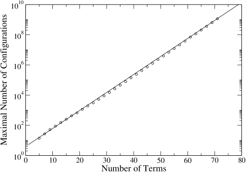
Figure 2: Lin-log plot of the maximal number of TM configurations from the pruned algorithm with increasing $n$.

The pruned algorithm is much too difficult to analyse exactly. So all we can give is a numerical calculation of the growth in the number of configurations with $n$. That is obtained by just running the SAW algorithm and measuring the maximal number of configurations generated for different values of $n$. The resulting graph is shown in fig. 2. The straight line, drawn as a guide to the eye, has slope $\lambda=\sqrt[4]{3}$ and thus corresponds to the exponential growth of the CEG algorithm. From this figure it is clear that the computational complexities of the two algorithms are almost identical. A closer look at the actual numbers does however reveal that the pruned algorithm appears to have a slightly higher value of $\lambda_{p}$. Indeed it appears that increasing $n$ by 8 increases the number of configurations by close to a factor of 10 (rather than the 9 expected if $\lambda_{p}=\sqrt[4]{3}$). This would mean that for the pruned algorithm $\lambda_{p}\approx\sqrt[8]{10}=1.3335\ldots$.

The observed value of $\lambda_{p}$ means that the CEG algorithm is asymptotically superior to the pruning algorithm, so that for very large values of $n$ it will be not only be faster but require less memory as well. However for small $n$ the pruning algorithm is highly competitive and can in fact use significantly less memory. This is because the CEG algorithm uses a two parameter generating function so memory requirements are $\propto n^{2}\lambda^{n}$. For the pruning algorithm memory growth is $\propto\lambda_{p}^{n}$, rather than what one may naively have thought $\propto n\lambda_{p}^{n}$ (see comments at the end of the previous section). More concretely, we can mention that the calculation in [6] of SAWs up to to $n=51$ required 10GB of memory. The pruning algorithm can do the same job using less than 150MB of memory.

2.5 Parallelization

The transfer-matrix algorithms used in the calculations of the finite lattice contributions are eminently suited for parallel computations. The bulk of the calculations for this paper were performed on the facilities of the Australian Partnership for Advanced Computing (APAC). The APAC facility is a HP Alpha server cluster with 125 ES45’s each with four 1 Ghz chips for a total of 500 processors in the compute partition. Each server node has at least 4 Gb of memory. Nodes are interconnected by a low latency high bandwidth Quadrics network.

The most basic concern in any efficient parallel algorithm is to minimise the communication between processors and ensure that each processor does the same amount of work and uses the same amount of memory. In practice one naturally has to strike some compromise and accept a certain degree of variation across the processors.

One of the main ways of achieving a good parallel algorithm using data decomposition is to try to find an invariant under the operation of the updating rules. That is we seek to find some property of the configurations along the boundary line which does not alter in a single iteration. The algorithm for the enumeration of SAWs is quite complicated since not all possible configurations occur due to pruning and an update at a given set of edges might change the state of an edge far removed, e.g., when two lower loop ends are joined we have to relabel one of the associated upper loop ends as a lower loop end in the new configuration. However, there is still an invariant since any edge not directly involved in the update cannot change from being empty to being occupied and vice versa. That is only the kink edges can change their occupation status. This invariant allows us to parallelise the algorithm in such a way that we can do the calculation completely independently on each processor with just two redistributions of the data set each time an extra column is added to the lattice. We have already used this scheme for SAPs [16] and lattice animals [15] and refer the interested reader to these publications for further detail. Our parallelisation scheme is also very similar to that used by Conway and Guttmann [6, 12].

2.6 Metric properties

In a recent paper [14] we demonstrated that one can use transfer matrix techniques to calculate the radius of gyration of SAPs. Below we show how this work can be extended to calculate the metric properties of SAWs.

2.6.1 Radius of gyrations

We define the radius of gyration according to the vertices of the SAW. Note that the number of vertices is one more than the number of steps. The radius of gyration of $n+1$ points at positions ${\bf r}_{i}$ is

$$(n+1)^{2}\langle R^{2}_{g}\rangle_{n}=\sum_{i>j}({\bf r}_{i}-{\bf r}_{j})^{2}=n\sum_{i}(x_{i}^{2}+y_{i}^{2})-2\sum_{i>j}(x_{i}x_{j}+y_{i}y_{j}).$$ (2.4)

This last expression is suitable for a transfer matrix calculation. We actually calculate the coefficients of the generating function (1.4b), $(n+1)^{2}c_{n}\langle R^{2}_{g}\rangle_{n}$. In order to do this we have to maintain five partial generating functions for each possible boundary configuration, namely

• $C(u)$, the number of (partially completed) SAWs.

• $X^{2}_{g}(u)$, the sum over SAWs of the squared components of the distance vectors.

• $X_{g}(u)$, the sum of the $x$-component of the distance vectors.

• $Y_{g}(u)$, the sum of the $y$-component of the distance vectors.

• $XY_{g}(u)$, the sum of the ‘cross’ product of the components of the distance vectors, that is, $\sum_{i>j}(x_{i}x_{j}+y_{i}y_{j})$.

As the boundary line is moved to a new position each target configuration $S$ might be generated from several sources $S^{\prime}$ in the previous boundary position. The partial generation functions are updated as follows, with $(x,y)$ being the coordinates of the newly added vertex:

$$C(u,S) = \sum_{S^{\prime}}u^{n^{\prime}}C(u,S^{\prime}),$$

$$X^{2}_{g}(u,S) = \sum_{S^{\prime}}u^{n^{\prime}}[X^{2}_{g}(u,S^{\prime})+\delta_{g}(x^{2}+y^{2})C(u,S^{\prime})],$$

$$X_{g}(u,S) = \sum_{S^{\prime}}u^{n^{\prime}}[X_{g}(u,S)+\delta_{g}xC(u,S^{\prime})],$$ (2.5)

$$Y_{g}(u,S) = \sum_{S^{\prime}}u^{n^{\prime}}[Y_{g}(u,S)+\delta_{g}yC(u,S^{\prime})],$$

$$XY_{g}(u,S) = \sum_{S^{\prime}}u^{n^{\prime}}[XY_{g}(u,S^{\prime})+\delta_{g}xX_{g}(u,S^{\prime})+\delta_{g}yY_{g}(u,S^{\prime})],$$

where $n^{\prime}$ is the number of steps added to the SAW and $\delta_{g}=0$ if the new vertex is empty (has degree 0), $\delta_{g}=1$ if the new vertex is occupied (has degree $>0$).

Finally, when valid SAWs are completed, the partial generating functions are added to running totals for each case, and the results for coefficients in the generating function for the radius of gyration is:

$$(n+1)^{2}c_{n}\langle R^{2}_{g}\rangle_{n}=n\langle X^{2}_{g}\rangle_{n}-2\langle XY_{g}\rangle_{n}.$$ (2.6)

2.6.2 End-to-end distance

The updating rules for the end-to-end distance are very similar to those for the radius of gyration except that we ‘count’ only the degree-1 vertices. We again maintain five partial generating functions for each possible boundary configuration, namely

• $C(u)$, the number of (partially completed) SAWs.

• $X^{2}_{e}(u)$, the sum over SAWs of the squared components of the end-point vectors.

• $X_{e}(u)$, the sum of the $x$-component of the end-point vectors.

• $Y_{e}(u)$, the sum of the $y$-component of the end-point vectors.

• $XY_{e}(u)$, the sum of the ‘cross’ product of the components of the end-point vectors.

The partial generation functions are updated as described above (2.6.1) except that the corresponding quantity $\delta_{e}=0$ if the new vertex has degree 0 or 2, while $\delta_{e}=1$ if the new vertex has degree 1.

The results for coefficients in the generating function for the end-to-end distance is:

$$c_{n}\langle R^{2}_{e}\rangle_{n}=\langle X^{2}_{e}\rangle_{n}-2\langle XY_{e}\rangle_{n}.$$ (2.7)

2.6.3 Mean-square monomer distance from end points

In order to calculate the mean-square distance of a monomer from the end points we have to introduce an additional partial generating function

• $XY_{m}(u)$, the sum of the ‘cross’ product of the components of the end-points and distance vectors.

This is updated as follows:

$$XY_{m}(u,S)=\sum_{S^{\prime}}u^{n^{\prime}}[XY_{m}(u,S^{\prime}) \!\!\!+\!\!\! \delta_{g}xX_{e}(u,S^{\prime})+\delta_{g}yY_{e}(u,S^{\prime})$$ (2.8)

$$\!\!\!+\!\!\! \delta_{e}xX_{g}(u,S^{\prime})+\delta_{e}yY_{g}(u,S^{\prime})].$$

The results for the coefficients in the generating function for the mean-square monomer distance from end points is :

$$c_{n}\langle R^{2}_{e}\rangle_{m}=(n-1)\langle X^{2}_{e}\rangle_{n}+2\langle X^{2}_{g}\rangle_{n}-2\langle XY_{m}\rangle_{n}.$$ (2.9)

2.7 Further details

Finally a few remarks of a more technical nature. The number of contributing configurations becomes very sparse in the total set of possible states along the boundary line and as is standard in such cases one uses a hash-addressing scheme. Since the integer coefficients occurring in the series expansion become very large, the calculation was performed using modular arithmetic [19]. This involves performing the calculation modulo various integers $p_{i}$ and then reconstructing the full integer coefficients at the end. The $p_{i}$ are called moduli and must be chosen so they are mutually prime, e.g., none of the $p_{i}$ have a common divisor. The Chinese remainder theorem ensures that any integer has a unique representation in terms of residues. If the largest absolute values occurring in the final expansion is $m$, then we have to use a number of moduli $k$ such that $p_{1}p_{2}\cdots p_{k}/2>m$. Since we are using a heavily loaded shared facility CPU time was more of an immediate limitation than memory. So we used the moduli $p_{0}=2^{62}$ and $p_{1}=2^{62}-1$, which allowed us to represent $p_{n}$ correctly just using these two moduli.

The calculation of the metric properties require a lot more memory for the generating functions, and involves multiplication with quite large integers, so in this case we used prime numbers of the form $2^{30}-r_{i}$ for the moduli $p_{i}$. Up to 4 primes were needed to represent the coefficients correctly.

We were able to extend the series for the square lattice SAW generating function from 51 terms to 71 terms using at most 100Gb of memory. The calculations requiring the most resource were at widths 24–29. These cases were done using 128 processors and took from 16 to 26 hours each. We also calculated the metric properties of SAWs up to length 59, thus extending these series from length 32 obtained previously using direct enumeration. In total the calculations used about 50000 CPU hours.

In table 2 we list the number of SAWs from length 52 to 71. The number of SAWs up to length 51 are tabulated in [12] and [1] (this paper also tabulates the metric properties and several other series). The numbers are also available from our home page.

Table 2: The number, $c_{n}$, of embeddings of $n$-step SAWs on the square lattice. Only terms for $n>51$ are listed.

$n$	$c_{n}$	$n$	$c_{n}$
52	37325046962536847970116	62	646684752476890688940276172
53	99121668912462180162908	63	1715538780705298093042635884
54	263090298246050489804708	64	4549252727304405545665901684
55	698501700277581954674604	65	12066271136346725726547810652
56	1853589151789474253830500	66	31992427160420423715150496804
57	4920146075313000860596140	67	84841788997462209800131419244
58	13053884641516572778155044	68	224916973773967421352838735684
59	34642792634590824499672196	69	596373847126147985434982575724
60	91895836025056214634047716	70	1580784678250571882017480243636
61	243828023293849420839513468	71	4190893020903935054619120005916

3 Analysis of the series

To obtain the singularity structure of the generating functions we used the numerical method of differential approximants [10]. The functions have critical points at $u_{c}$ with exponents as in (1.1b)-(1.5b). Our main objective is to obtain accurate estimates for the connective constant $\mu$ and the critical exponents $\gamma$ and $\nu$. In particular we confirm to a very high degree of precision the conjectured exact values of the exponents.

Once the exact values of the exponents have been confirmed we turn our attention to the “fine structure” of the asymptotic form of the coefficients. In particular we are interested in obtaining accurate estimates for the amplitudes $A$, $C$, $D$ and $E$. We do this by fitting the coefficients to the form given by (1.1a)-(1.5a). In this case our main aim is to test the validity of the predictions for the amplitude combinations mentioned in the Introduction.

3.1 The SAW generating function

In Table 3 we list estimates for the critical point $u_{c}$ and exponent $\gamma$ of the series for the square lattice SAW generating function. The estimates were obtained by averaging values obtained from second and third order differential approximants. For each order $L$ of the inhomogeneous polynomial we averaged over those approximants to the series which used at least the first 60 terms of the series. The error quoted for these estimates reflects the spread (basically one standard deviation) among the approximants. Note that these error bounds should not be viewed as a measure of the true error as they cannot include possible systematic sources of error. Based on these estimates we conclude that $u_{c}=0.379052274(4)$ and $\gamma=1.343745(15)$. The estimate for $u_{c}$ is compatible with the much more accurate estimate $u_{c}=0.37905227773(7)$ obtained from the analysis of the SAP generating function [16]. The analysis adds further support to the already convincing evidence that the critical exponent $\gamma=43/32=1.34375$ exactly. However, we do observe that both the central estimates for both $u_{c}$ and $\gamma$ are systematically very slightly lower than the expected values.

Table 3: Estimates for the critical point $u_{c}$ and exponent $\gamma$ obtained from second and third order differential approximants to the series for square lattice SAW generating function. $L$ is the order of the inhomogeneous polynomial.

$L$	Second order DA		Third order DA
	$u_{c}$	$\gamma$	$u_{c}$	$\gamma$
0	0.3790522679(60)	1.343735(29)	0.3790522735(11)	1.3437397(18)
2	0.3790522729(11)	1.3437388(23)	0.3790522752(11)	1.3437427(22)
4	0.3790522720(13)	1.3437387(32)	0.3790522756(27)	1.3437438(61)
6	0.37905227192(81)	1.3437369(24)	0.3790522751(27)	1.3437429(61)
8	0.3790522733(15)	1.3437395(24)	0.3790522752(27)	1.3437434(63)
10	0.3790522739(30)	1.343744(12)	0.3790522751(22)	1.3437430(39)
12	0.3790522740(19)	1.3437404(34)	0.3790522755(63)	1.343748(11)
14	0.3790522738(13)	1.3437398(22)	0.3790522738(25)	1.3437406(37)
16	0.3790522739(12)	1.3437403(20)	0.3790522733(39)	1.3437408(53)
18	0.3790522734(14)	1.3437398(25)	0.3790522753(19)	1.3437433(41)
20	0.3790522749(32)	1.3437437(87)	0.3790522755(25)	1.3437435(78)

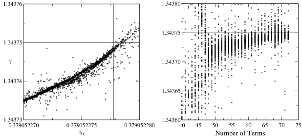
Figure 3: Estimates for $\gamma$ vs. $u_{c}$ (left panel) and $\gamma$ vs. the number of terms used by the differential approximant (right panel).

When analysing series it is always problematic to get a reliable error estimate. So in trying to confirm, as we are here, the exact value of a critical exponent, it is often useful to plot the behaviour of the estimates against both $u_{c}$ and the number of terms used by the differential approximants. In this way it often possible to gauge more clearly whether or not the high-order approximants have settled down to the limiting value of the true exponent. In fig. 3 we carry out such an analysis. Each point in the left panel correspond to estimates for $u_{c}$ and $\gamma$ obtained from a third order differential approximant. The right panel shows the estimates of $\gamma$ but now plotted against the number of terms used by the differential approximant. The straight lines indicate the expected exact value of $\gamma$ and the highly accurate estimate of $u_{c}$ obtained from the analysis of the SAP series. From the plot in the right panel we can see that the estimates of $\gamma$ still exhibits a certain up wards drift as the number of terms in the approximants increase. So the estimates of $\gamma$ have not yet settled at their limiting value, but there can be no doubt that the predicted exact value of $\gamma$ is fully consistent with the estimates. In the left panel we observe that the $(u_{c},\gamma)$-estimates fall in a narrow range. Note that this range does not include the intersection point between the exact $\gamma$ and the precise $u_{c}$ estimate. This is probably a reflection of the lack of ‘convergence’ to the true limiting values. This view is further supported by repeating the plot of fig. 3, but only using those approximants using a number of terms is a prescribed interval, which we choose as 51-55, 56-60, 61-65, and 65-71. This corresponds to looking at the plots one would have obtained had the series only been known up to the lengths 55, 60, 65 and 71, respectively. These plots show that as more terms are included the $(u_{c},\gamma)$-estimates move closer and closer to the expected intersection point. This drift is again a clear indication that the estimates have not yet settled at the true limiting values.

3.2 The metric properties

We now turn our attention to the metric properties. The generating functions are expected to have a singularity at $u_{c}$ where the end-to-end distance (1.3b) has exponent $\gamma+2\nu=91/32=2.84375$, the radius of gyration (1.4b) has exponent $\gamma+2\nu+2=155/32=4.84375$, and the mean square monomer distance from the end points (1.5b) has exponent $\gamma+2\nu+1=123/32=3.84375$. In table 4 we list the estimates obtained from a differential approximant analysis of these series. In summary we see that applying differential approximants to the metric series yields for the end-to-end distance $u_{c}=0.37905205(15)$ and $2\nu=2.8434(4)$, the radius of gyration yields $u_{c}=0.379052230(5)$ and $2\nu+2=4.84360(2)$, and the monomer distance yields $u_{c}=0.3790521(1)$ and $2\nu+1=3.84335(15)$. We immediately note that the exponent estimates are systematically lower that the expected exact values. Only the end-to-end distance is marginally consistent with the expected value, while there is a considerable discrepancy between the radius of gyration estimate and the expected value (similar though less pronounced for the monomer distance). However, we also note that the $u_{c}$ estimates are quite far from the SAP estimate (in which we have considerable confidence) $u_{c}=0.37905227773(7)$. So obviously the metric series are not that well behaved and might have large corrections to scaling.

Table 4: Estimates for the critical point $u_{c}$ and critical exponents obtained from second and third order differential approximants to the series for the end-to-end distance, radius of gyration, and monomer distance from the end point.

$\mathcal{R}_{e}(u)$
$L$	Second order DA		Third order DA
	$u_{c}$	$\gamma+2\nu$	$u_{c}$	$\gamma+2\nu$
0	0.379052003(90)	2.84324(62)	0.379052101(69)	2.84333(19)
2	0.379051985(57)	2.84301(96)	0.379052116(58)	2.84336(11)
4	0.379052046(81)	2.84345(18)	0.379052113(75)	2.84336(10)
6	0.379052034(80)	2.84329(39)	0.379052119(86)	2.84334(19)
8	0.379052054(69)	2.8430(19)	0.379052115(75)	2.84337(33)
10	0.379052035(67)	2.84329(23)	0.379052138(66)	2.84338(11)
$\mathcal{R}_{g}(u)$
$L$	Second order DA		Third order DA
3	$u_{c}$	$\gamma+2\nu+2$	$u_{c}$	$\gamma+2\nu+2$
0	0.3790522317(19)	4.8436019(22)	0.3790522289(11)	4.8435986(13)
2	0.3790522317(26)	4.8436017(29)	0.3790522295(10)	4.8435992(11)
4	0.3790522324(41)	4.8436024(45)	0.3790522289(22)	4.8435986(23)
6	0.3790522290(94)	4.843598(11)	0.3790522284(23)	4.8435980(26)
8	0.379052225(15)	4.843595(16)	0.3790522294(43)	4.8435992(48)
10	0.3790522282(21)	4.8435978(24)	0.3790522301(20)	4.8436000(24)
$\mathcal{R}_{m}(u)$
$L$	Second order DA		Third order DA
	$u_{c}$	$\gamma+2\nu+1$	$u_{c}$	$\gamma+2\nu+1$
0	0.379052045(58)	3.84321(11)	0.379052131(39)	3.843345(61)
2	0.379052056(37)	3.843256(63)	0.379052118(57)	3.843327(93)
4	0.379052044(70)	3.84323(10)	0.379052107(68)	3.84332(10)
6	0.379052050(73)	3.84322(10)	0.379052088(51)	3.843281(96)
8	0.379052081(99)	3.84329(17)	0.379052081(52)	3.843274(95)
10	0.379052069(95)	3.84326(17)	0.379052135(55)	3.843370(86)

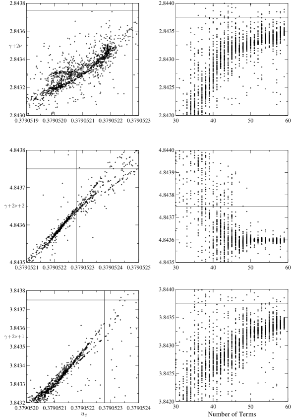
Figure 4: Plots of estimates for the critical exponents vs. the critical point (left panels) and critical exponents vs. number of terms (right panels) obtained form third order differential approximants to the generating functions $\mathcal{R}_{e}(u)$ (top panels), $\mathcal{R}_{g}(u)$ (middle panels) and $\mathcal{R}_{m}(u)$ (bottom panels).

As for the SAW generating function, we find it useful to plot the estimates for the critical exponents vs. $u_{c}$ and the number of terms. This we have done in fig. 4. Clearly the estimates from the end-to-end distance have not yet converged and it is quite possible that the exponent estimates will eventually converge to the expected value (see top left panel). Also in the top right panel it is quite possible that the estimates will approach the point given by the intersection of the exact exponent value and the precise $u_{c}$ value. The behaviour of the estimates for radius of gyration and monomer distance series are far more unsettling. In particular, the exponent estimates from the radius of gyration series appears well converged to a value $4.84360$ with a narrow spread which clearly does not include the expected exact value $4.84375$ and in the plot of the exponent vs. $u_{c}$ (middle left panel) the estimates are quite far from the expected intersection. Similar remarks hold for the monomer distance (bottom panels) though convergence and discrepancy with expected values is less pronounced. Furthermore, the behaviour of the radius of gyration series is very different to the other series. In particular we note that in the plots of the exponents vs. the number of terms (left panels) the estimates from the end-to-end and monomer distance seems to increase monotonically to wards the expected value, while the estimates from the radius of gyration starts out above the expected value, then cross the expected value before apparently settling below the expected value. This behaviour is quite puzzling. Let us just note that if we look at the similar plots for the SAW generating function (fig. 3) it is clear that convergence has not been achieved at $n=59$ and not yet even at $n=71$. It would therefore be surprising if we should not see a further drift in the exponent estimates for the metric properties with longer series.

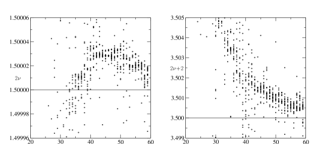
Figure 5: Plots of estimates of the critical exponents versus the number of terms obtained form third order differential approximants to the functions $\mathcal{R}_{e}(u)/(u\mathcal{C}(u))$ (left panel) and $\mathcal{R}_{g}(u)/(u\mathcal{C}(u))$ (right panel).

Fortunately, we have the possibility of analysing other series involving the metric properties. We can look directly at the generating function with coefficients $\langle R^{2}_{e}\rangle_{n}$, and so on. While this has the advantage that we know that these series have a critical point at $u_{c}=1$ it turns out that the estimates of the critical exponents, $-2\nu-1$ in all cases, behave in exactly the same manner as the series for the original generating functions. A second, and as we shall see much more successful approach, is to take the original series and divide them by the SAW generating function. That is we study the series $\mathcal{R}_{e}(u)/(u*\mathcal{C}(u))\propto(u-u_{c})^{-2\nu}$, and so on, where again $u_{c}=1/\mu$. We won’t go through all the details here. Suffice to say that applying differential approximants to the resulting series yields for the end-to-end distance series $u_{c}=0.37905229(2)$ and $2\nu=1.50002(3)$, the radius of gyration series yields $u_{c}=0.3790526(4)$ and $2\nu+2=3.5006(4)$, and the monomer distance series yields $u_{c}=0.3790524(2)$ and $2\nu+1=2.5002(4)$. This clearly confirms that $\nu=3/4$, exactly. We notice that the error estimates of the modified series is quite different to the original series. The original end-to-end series has the largest error estimate of the three while the modified end-to-end series has the smallest error estimate. The opposite happens for the radius of gyration series. The quite different behaviour of these series, as compared to the original ones, is probably even more clearly illustrated in fig. 5 where we have plotted the exponent estimates vs. the number of terms for the modified end-to-end and radius of gyration series. Clearly, the estimates from both of these series appear not yet to have settled at their limiting values, but it would seem that they are converging to wards the expected exponent values. Note the very different behaviour of the original and modified radius of gyration series. So obviously dividing by the SAW generating function has a dramatic effect on the metric series. We can only guess that this procedure leads to modifications in the correction-to-scaling behaviour thus altering dramatically the convergence properties of the series.

3.3 Non-physical singularities

The generating functions have singularities on the negative axis at $u_{-}=-1/\mu=-x_{c}$. The exponents at $u_{-}$ are compatible with simple exact values. For the SAW generating function the exponent is $1/2$, for the end-to-end generating function (1.3b) the exponent is also $1/2$, for the radius of gyration generating function (1.3b) the exponent is $-3$, while for the monomer distance generating function (1.5b) the exponent is $-2$.

3.4 Correction-to-scaling exponent

The correction-to-scaling exponent for SAWs is exhaustively studied in a recent paper [1] using series analysis and Monte Carlo simulations. In particular we performed a very careful and detailed analysis of the of the 59 step series for the square lattice SAW counts and metric properties and a 40 step series for the triangular lattice. In that study of the SAW correction-to-scaling exponents, a consistent picture emerged. We presented compelling evidence that the first non-analytic correction term in the generating function for SAWs and SAPs is $\Delta_{1}=3/2$, as predicted by Nienhuis [25, 26]. We found no evidence for the presence of an exponent $\Delta_{1}=11/16$ in SAWs and SAPs on the square and triangular lattices, as proposed by Saleur [30].

Our method of analysis, both here and in [1], is based on direct fitting to the expected asymptotic form. Obviously (1.1a) only gives the leading term in the asymptotic expansion. We have to add in both analytic and non-analytic corrections to scaling. Furthermore, we have to take account of the presence of the singularity at $u_{-}=-1/\mu$. We thus expect $c_{n}$ to have an asymptotic expansion of the form

$$c_{n}\sim\mu^{n}n^{\gamma-1}[a_{0}+\sum_{i=1}^{k}\frac{a_{i}}{n^{\Delta_{i}}}]+(-\mu)^{n}n^{\alpha-2}[b_{0}+\sum_{i=1}^{m}\frac{b_{i}}{n^{\Gamma_{i}}}],$$ (3.1)

where $\alpha$ is the critical exponent occurring in the polygon generating function.

We estimate the coefficients $a_{i}$ and $b_{i}$, by inserting the estimated value of $\mu,$ the exact values of $\gamma$ and $\alpha$, and assumed values of $\Delta_{i}$ and $\Gamma_{i}$. The coefficients can then be fitted to the assumed asymptotic form by solving a system of linear equations. By steadily increasing the number of series coefficients, many estimates for the $\{a_{i}\}$ and $\{b_{i}\}$ are found. Provided the different estimates are consistent over series of different lengths we assume that they provide an acceptably accurate estimate of the actual asymptotic coefficients.

A noteworthy feature of the method is that, if a blatantly false exponent is given as input (for example, specifying $\Delta_{1}=1/2$ for the two-dimensional SAW), the sequence of amplitude estimates for the term corresponding to that exponent will converge rapidly to zero, giving a very strong signal that the exponent in question is absent. It was this feature which was used to rule out $\Delta_{1}=11/16$.

Note that one would expect a whole sequence $\Delta_{j}>\Delta_{1}$ of non-analytic corrections to scaling, as well as so-called mixing terms involving the exponents $\gamma$ and $\alpha$ (see [1] for details). The first expected mixing term would give a contribution $n^{-59/32}$ [1]. However, in practice this is indistinguishable from the $n^{-2}$ term. Higher order corrections can likewise not be detected since they make contributions well beyond the range of reasonable extrapolation.

3.5 Amplitudes

In our paper [1] we also obtained accurate amplitude estimates. Here we shall therefore only briefly review these results then report on the slightly improved estimates for the amplitudes of the SAW counts based on the extended 71 term series.

Given the value for the non-analytic correction-to-scaling exponent we more concretely choose to fit fit to the form used in [1]:

$$c_{n} \sim \mu^{n}n^{11/32}[a_{0}+a_{1}/n+a_{2}/n^{3/2}+a_{3}/n^{2}+a_{4}/n^{5/2}+\cdots]$$ (3.2)

$$+ (-1)^{n}\mu^{n}n^{-3/2}[b_{0}+b_{1}/n+b_{2}/n^{2}+b_{3}/n^{3}+\cdots].$$

Fitting to this form we found [1], using the 59 term SAW counts, $a_{0}=A=1.1770425(5)$ as well as reasonably accurate estimates for $a_{1}$–$a_{3}$ and $b_{0}$–$b_{2}$. For the metric properties we found $C=0.77124(8)$, $D=0.108227(58)(5)$ and $E=0.33913(14)$. A similar analysis of the triangular lattice data yielded $A=1.183966(2)$, $C=0.71176(66)$, $D=0.09987(5)$ and $E=0.3130(5)$.

Table 5: Estimates of universal amplitude combinations on some two-dimensional lattices.

Lattice	$D/C$	$E/C$	$BC/\sigma a_{0}$	$F$
Square [1, 16]	0.140299(6)	0.439647(6)	0.21683(4)	-0.000024(28)
Triangular [1, 17]	0.140296(6)	0.439649(9)	0.2169(2)	-0.000036(34)
Honeycomb [21]	0.1403(1)	0.4397(2)	0.2170(3)	-0.00013(67)
Kagomé [22, 23]	0.140(1)	0.440(1)	0.2144(25)	-0.0015(47)

The ratios $D/C$ and $E/C$ were also estimated by direct extrapolation of the relevant quotient sequence, using the following method [27]: Given a sequence $\{a_{n}\}$ defined for $n\geq 1$, assumed to converge to a limit $a_{\infty}$ with corrections of the form $a_{n}\sim a_{\infty}(1+b/n+\ldots)$, we first construct a new sequence $\{h_{n}\}$ defined by $h_{n}=\prod_{m=1}^{n}a_{m}$. The generating function $\sum h_{n}x^{n}\sim(1-a_{\infty}x)^{-(1+b)}$. Estimates for $a_{\infty}$ and the parameter $b$ can then be obtained from differential approximants. In this way, we obtained the estimates [1], $D/C=0.140299(6)$ and $E/C=0.439647(6)$ for the square lattice and $D/C=0.140296(6)$ and $E/C=0.439649(9)$ for the triangular lattice.

The amplitude estimates leads to a high precision confirmation of the CSCPS relation (1.6) $F=0.000024(25)$.

In Table 5 we have listed the estimates of various universal amplitude combinations, obtained from the work reported in this paper and elsewhere. As can be seen the estimates for all lattices are in perfect agreement strongly confirming the universality of the various combinations.

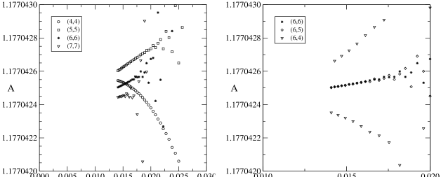
Figure 6: Plots of estimates for the leading amplitude $A$ from various fits of $c_{n}$ to the assumed asymptotic expansion (3.1).

Finally we turn to the estimation of the amplitude $A$ using the new extended 71 term series. As in previous work [14, 16] we find it very useful to plot the amplitude estimates vs. $1/n$ where $c_{n}$ is the last coefficient used by the fit. In fig. 6 we plot the estimates for the leading amplitude $A$ from various fits. The legend numbers $(k,m)$ indicates the number of terms used in the fit by each part of the asymptotic expansion (3.1), using the exponents given in the explicit form (3.2). From the left panel we see a consistent trend emerging. As the number of terms used in $(k,k)$-fits is increased we see that the estimates settle down and that fits using more terms display less curvature. We take this as a clear indication that the fitting procedure is robust and that the assumed asymptotic expansion is correct. The fits using 5, 6, and 7 terms each can clearly be extrapolated to a value $A=1.770423(1)$. In the right panel we plot amplitude estimates from $(k,m)$-fits with $k=6$ and $m=6$, 5 and 4. We do this merely to point out that clearly only $(k,m)$-fits with $m$ close to $k$ are reliable. The $(6,4)$-fit displays a pronounced oscillatory behaviour.

4 Summary and conclusion

We have presented a new algorithm for the enumeration of self-avoiding walks. Numerical data show that it has computational complexity only slightly worse than the Conway-Enting-Guttmann algorithm [5]. This means that the CEG algorithm will be superior for enumerating very long SAWs. However, the new algorithm uses much less memory at shorter lengths and remains competitive at lengths attainable at present and in the foreseeable future. Furthermore the new algorithm can be used to calculate metric properties such as the end-to-end distance, radius of gyration, and average distance of monomers from the end points. We have used the algorithm to extend the series for the number of SAWs on the square lattice up to 71 steps and calculate the metric properties of SAWs up to 59 steps.

Analysis of the series yielded estimates of the critical exponents $\gamma$ and $\nu$ which confirmed to a high degree of accuracy the predicted exact values $\gamma=43/32$ and $\nu=3/4$. We reported on results from a comprehensive analysis [1] of the series providing very firm and convincing evidence that the leading non-analytic correction to scaling is $\Delta_{1}=3/2$, as well as giving accurate estimates for the critical amplitudes. The amplitude estimates led to a high precision confirmation of the CSCPS relation (1.6) $F=0$.

5 Acknowledgments

It is a pleasure to thank Tony Guttmann for a careful reading of the manuscript and many helpful suggestions. The calculations presented in this paper would not have been possible without a generous grant of computer time on the server cluster of the Australian Partnership for Advanced Computing (APAC). We also used the computational resources of the Victorian Partnership for Advanced Computing (VPAC). We gratefully acknowledge financial support from the Australian Research Council.

References

- [1] Caracciolo S, Guttmann A J, Jensen I, Pelissetto A, Rogers A N and Sokal A D 2004 Correction-to-scaling exponents for two-dimensional self-avoiding walks in preparation
- [2] Caracciolo S, Pelissetto A and Sokal A D 1990 Universal distance ratios for two-dimensional self-avoiding walks: corrected conformal invariance predictions J. Phys. A: Math. Gen. 23 L969–L974
- [3] Cardy J L and Guttmann A J 1993 Universal amplitude combinations for self-avoiding walks, polygons and trails J. Phys. A: Math. Gen. 26 2485–2494
- [4] Cardy J L and Saleur H 1989 Universal distance ratios for two-dimensional polymers J. Phys. A: Math. Gen. 22 L601–L604
- [5] Conway A R, Enting I G and Guttmann A J 1993 Algebraic techniques for enumerating self-avoiding walks on the square lattice J. Phys. A: Math. Gen. 26 1519–1534
- [6] Conway A R and Guttmann A J 1996 Square lattice self-avoiding walks and corrections to scaling Phys. Rev. Lett. 77 5284–5287
- [7] Delest M P and Viennot G 1984 Algebraic languages and polyominoes enumeration Theor. Comput. Scie. 34 169–206
- [8] Enting I G 1980 Generating functions for enumerating self-avoiding rings on the square lattice J. Phys. A: Math. Gen. 13 3713–3722
- [9] Enting I G and Guttmann A J 1996 On the solvability of some statistical mechanics systems Phys. Rev. Lett. 76 344–377
- [10] Guttmann A J 1989 Asymptotic analysis of power-series expansions in Phase Transitions and Critical Phenomena (eds. C Domb and J L Lebowitz) (New York: Academic) vol. 13 pp. 1–234
- [11] Guttmann A J 2000 Indicators of solvability for lattice models Discrete Math. 217 167–189
- [12] Guttmann A J and Conway A R 2001 Square lattice self-avoiding walks and polygons Ann. Comb. 5 319–345
- [13] Guttmann A J and Yang Y S 1990 Universal distance ratios for 2d saws: series results J. Phys. A: Math. Gen. 23 L117–L119
- [14] Jensen I 2000 Size and area of square lattice polygons J. Phys. A: Math. Gen. 33 3533–3543
- [15] Jensen I 2003 Counting polyominoes: A parallel implementation for cluster computing in Computational Science – ICCS 2003 (eds. P M A Sloot, D Abramson, A V Bogdanov, J J Dongarra, A Y Zomaya and Y E Gorbachev) (Berlin: Springer) vol. 2659 of Lecture Notes in Computer Science pp. 203–212
- [16] Jensen I 2003 A parallel algorithm for the enumeration of self-avoiding polygons on the square lattice J. Phys. A: Math. Gen. 36 5731–5745
- [17] Jensen I 2004 Self-avoiding walks and polygons on the triangular lattice In preparation
- [18] Jensen I and Guttmann A J 1999 Self-avoiding polygons on the square lattice J. Phys. A: Math. Gen. 32 4867–4876
- [19] Knuth D E 1969 Seminumerical Algorithms. The Art of Computer Programming, Vol 2. (Reading, Mass: Addison Wesley)
- [20] Knuth D E 2001 Polynum and Polyslave the program is available from Knuth’s Home-page at http://Sunburn.Stanford.EDU/~knuth/programs.html#polyominoes
- [21] Lin K Y 2000 Universal amplitude combinations for self-avoiding walks and polygons on the honeycomb lattice Physica A 275 197–206
- [22] Lin K Y and Huang J X 1995 Universal amplitude ratios for self-avoiding walks on the kagome lattice J. Phys. A: Math. Gen. 28 3641–3643
- [23] Lin K Y and Lue S J 1999 Universal amplitude combinations for self-avoiding polygons on the kagome lattice Physica A 270 453–461
- [24] Madras N and Slade G 1993 The self-avoiding walk (Boston: Birkhäuser)
- [25] Nienhuis B 1982 Exact critical point and critical exponents of O models in two dimensions Phys. Rev. Lett. 49 1062–1065
- [26] Nienhuis B 1984 Critical behavior of two-dimensional spin models and charge asymmetry in the coulomb gas J. Stat. Phys. 34 731–761
- [27] Owczarek A L, Prellberg T, Bennett-Wood D and Guttmann A J 1994 Universal distance ratios for interacting two-dimensional polymers J. Phys. A: Math. Gen. 27 L919–L925
- [28] Privman V and Redner S 1985 Tests of hyperuniversality for self-avoiding walks J. Phys. A: Math. Gen. 18 L781–L788
- [29] Richard C, Guttmann A J and Jensen I 2001 Scaling function and universal amplitude combinations for self-avoiding polygons J. Phys. A: Math. Gen. 34 L495–L501
- [30] Saleur H 1987 Conformal invariance for polymers and percolation J. Phys. A: Math. Gen. 20 455–470