Strong Coupling Theory for Interacting Lattice Models

Abstract

We develop a strong coupling approach for a general lattice problem. We argue that this strong coupling perspective represents the natural framework for a generalization of the dynamical mean field theory (DMFT). The main result of this analysis is twofold: 1) It provides the tools for a unified treatment of any non-local contribution to the Hamiltonian. Within our scheme, non-local terms such as hopping terms, spin-spin interactions, or non-local Coulomb interactions are treated on equal footing. 2) By performing a detailed strong-coupling analysis of a generalized lattice problem, we establish the basis for possible clean and systematic extensions beyond DMFT. To this end, we study the problem using three different perspectives. First, we develop a generalized expansion around the atomic limit in terms of the coupling constants for the non-local contributions to the Hamiltonian. By analyzing the diagrammatics associated with this expansion, we establish the equations for a generalized dynamical mean-field theory (G-DMFT). Second, we formulate the theory in terms of a generalized strong coupling version of the Baym-Kadanoff functional. Third, following Pairault, Sénéchal, and Tremblaytramb , we present our scheme in the language of a perturbation theory for canonical fermionic and bosonic fields and we establish the interpretation of various strong coupling quantities within a standard perturbative picture.

I Introduction

Understanding strongly correlated electron systems represents a major challenge in solid state physics. Dynamical mean-field theory (for a review see Ref.review, ) has emerged as a powerful tool to address this challenge. Within this approach, the lattice problem for an interacting electron system is mapped onto a quantum impurity problem with a “bath” determined self-consistentlydmft1 . In its simple form, the construction becomes exact in the limit of infinite lattice coordination as shown in Ref. dmft0, . In addition, several generalizations of the approach, such as the extended DMFTedmft1 ; edmft2 ; edmft3 ; edmft4 ; edmft5 and the DMFT treatment of correlated hoppingschill ; shvaik , requiring different scalings of the parameters in the Hamiltonian, have been presented.

More generally, DMFT is a tool with strong computational power, and provides valuable insight into the physics of strongly-correlated electrons. In the case of simple model Hamiltonians with purely local interactions, such as the Hubbard model, it was able to provide a consistent description for several non-perturbative properties such as, for example, the Mott-Hubbard metal insulator transitionreview . Currently, many efforts are made to extend the DMFT approach in order to make it suitable in addressing more realistic problems.

The purpose of this work is to develop a strong coupling approach for interacting lattice problems. Within this approach, we construct a systematic generalization of the DMFT technique capable of describing any non-local term of a generic lattice Hamiltonian. The present formulation has several advantages. First, it unifies various DMFT schemes. For example, the treatment of correlated hoppingschill ; shvaik , the single site DMFT of the Hubbard model (see Section III), and the extended DMFTedmft1 ; edmft2 ; edmft3 ; edmft4 ; edmft5 are all limiting cases of this unified approach. Second, besides unifying different DMFT schemes, this formulation is sufficiently general to be a starting point for expansions around DMFT. One possibility is described in the Appendix. In addition, the formulation in terms of Hubbard operators makes it an ideal framework for a DMFT based renormalization group approach  along the lines of Ref. rga, . Third, being based on an expansion around the atomic limit, it provides new and valuable insight into the diagrammatics underlying cluster DMFT schemes, which will be a subject of a subsequent publication.

The central result of this work is the formulation of a perturbation theory, for a general Hamiltonian of the form

$$H=H_{0}+H_{1},$$ (1)

containing a local term, $H_{0}$, and a non-local one, $H_{1}$. In terms of Hubbard operators, $X_{i}^{\alpha\beta}$, we can write the two contributions as

$$H_{0}=\sum_{i}\sum_{\alpha}\lambda_{\alpha}X_{i}^{\alpha\alpha},$$ (2)

and

$$H_{1}=\sum_{i\neq j}\sum_{\alpha,\beta,\alpha^{\prime},\beta^{\prime}}E_{ij}^{\alpha\beta\alpha^{\prime}\beta^{\prime}}X_{i}^{\alpha\beta}X_{j}^{\alpha^{\prime}\beta^{\prime}}.$$ (3)

In these equations $\alpha,\beta,\alpha^{\prime}$ and $\beta^{\prime}$ represent single-site states. For simplicity, we consider the case of spin $\frac{1}{2}$ fermions, so that for each site $i$ there will be four states $|\alpha\rangle$: $|0\rangle$ (empty site), $|\uparrow\rangle$ (single occupied site with spin up), $|\downarrow\rangle$ (single occupied site, spin down), and $|2\rangle$ (double occupied site). The Hubbard operators $X_{i}^{\alpha\beta}$ describe transitions between these states. These operators have a fermionic character if the occupation numbers of the states $\alpha$ and $\beta$ differ by one, and bosonic character otherwise. The algebra of the Hubbard operators is defined by the multiplication rule

$$X_{i}^{\alpha\beta}X_{i}^{\beta^{\prime}\alpha^{\prime}}=\delta_{\beta\beta^{\prime}}X_{i}^{\alpha\alpha^{\prime}},$$ (4)

together with the conserving condition

$$\sum_{\alpha}X_{i}^{\alpha\alpha}=1,$$ (5)

and the commutation relation

$$[X_{i}^{\alpha\beta}X_{j}^{\beta^{\prime}\alpha^{\prime}}]_{\pm}=\delta_{ij}(\delta_{\beta\beta^{\prime}}X_{i}^{\alpha\alpha^{\prime}}\pm\delta_{\alpha\alpha^{\prime}}X_{i}^{\beta^{\prime}\beta}).$$ (6)

In Eq. (6) the anticommutator is used if both operators are fermionic and the commutator otherwise. The canonic fermion operators $c_{i\sigma}$ can be expressed in terms of Hubbard operators as

$$c_{i\sigma}=X_{i}^{0\sigma}+\sigma X_{i}^{\sigma 2}.$$ (7)

The parameters $\lambda_{\alpha}$ in Eq. (2) represent the single-site energies and will be determined, in general, by the chemical potential, $\mu$, the on-site Hubbard interaction, $U$, and the external fields. The coupling constants $E_{ij}^{\alpha\beta\alpha^{\prime}\beta^{\prime}}$ may include contributions coming, for example, from hopping, $t_{ij}$, spin-spin interaction, $J_{ij}$, or non-local Coulomb interaction, $V_{ij}$. Within the present approach, all these contributions are treated on equal footing, and we can regard $E_{ij}^{\alpha\beta\alpha^{\prime}\beta^{\prime}}$ as generalized “hopping” matrix elements.

Our main object of interest is the Green’s function of the Hubbard operators. However, the theory is expressed naturally in terms of a generalized irreducible two-point cumulant, M, and a dressed hopping, ${\cal E}$. Using the language of a standard field theory (see the Appendix), we interpret M as a generalized self energy and ${\cal E}$ as the corresponding Green’s function associated with a set of auxiliary canonical fermionic and bosonic fields, and show that they have a clear diagrammatic interpretation in the locator expansion. In addition, our formulation contains the average ${\mbox{Q}}=\langle X\rangle$ of the Hubbard operator, which can be viewed as a generalized “magnetization”, together with a generalized effective “magnetic” field, h, represented, in the language of the standard field theory, by the mean value of the auxiliary field. Formally, the relationship between these quantities and the central object of the theory,  G, is given by the equations:

$$G=\langle\langle XX\rangle\rangle-\langle X\rangle\langle X\rangle=(M^{-1}-E)^{-1},$$

and

$${\cal E}=E(1-ME)^{-1}.$$

where E represents the bare coupling constants.

Next, we introduce the functional

$$\Gamma[{\cal E},Q]=-\mbox{Tr}~{}\ln[1-ME]-\mbox{Tr}[M{\cal E}]-\frac{1}{2}QEQ+\Psi[{\cal E},Q],$$

where $\Psi$ represents a generalized Baym-Kadanoff-type functional that can be obtained as a sum of all vacuum-to-vacuum skeleton diagrams. Using this functional perspective, we can view ${\cal E}$ and M, as well as Q and h, as pairs of conjugate quantities and we have $\delta\Psi/\delta{\cal E}=M$ and $\delta\Psi/\delta Q=h$, where the effective “magnetic” field can be expressed as $h=EQ$.

The single site dynamical mean field theory is a local approximation for  $\mbox{M}\approx\mbox{M}_{loc}$, which can be obtained as a stationarity condition for the functional $\Gamma$. This condition translates into a self-consistent impurity problem defined by the statistical operator

$$\hat{\rho}_{imp}=e^{-\beta H_{0}^{imp}}\hat{T}\exp\left\{-\int_{0}^{\beta}X(\tau)\Delta(\tau-\tau^{\prime})X(\tau^{\prime})+h_{imp}(\tau)X(\tau)\right\},$$

where $h_{imp}$ represents an external field and $\Delta$ the hybridization. These quantities are subjected to the self-consistency conditions:

$$\frac{1}{N}\sum_{k}~{}[M_{loc}^{-1}(i\omega_{n})-E(k)]^{-1}=[M_{loc}^{-1}(i\omega_{n})-\Delta(i\omega_{n})]^{-1},$$

and

$$h_{imp}+\Delta(0)\langle X\rangle=E\langle X\rangle.$$

The strategy that we use in presenting our G-DMFT scheme consists in constructing three formally distinct formulations. On the one hand, this allows us to establish the equivalence of these approaches to the problem of correlated electrons and to extract a generalized unitary picture. On the other hand, these various angles clearly reveal the aspects that are relevant for the possible extensions of the theory. The natural starting point for our construction is given by a generalized expansion around the atomic limit. This expansion, in terms of the coupling constants of the non-local contributions to the Hamiltonian, is derived in Sec. II. The technique is characterized by a close formal analogy with the “canonical” perturbation expansion in terms of inter-site hopping. Consequently, we will focus on the new aspects generated by the description of the problem in terms of Hubbard operators, the main goal being to obtain the relation between the Green’s function for the Hubbard operators and the irreducible two-point cumulant. Using this relation, we derive in Sec. III the generalized DMFT equations. A simple illustration of the implementation of our scheme is given for the Hubbard model. In Sec. IV we formulate the theory in terms of a functional of the renormalized “hopping”˙The generalized DMFT equations are shown to be the result of a simple local approximation on a generalized Baym-Kadanoff-type functional. An alternative derivation is described in the Appendix. By decoupling the non-local term via a Hubbard-Stratonovich transformation, we formulate the theory in terms of a set of canonical fermionic and bosonic fields. In this language, the standard treatment based on Wick’s theorem applies. A possibility of expanding around the DMFT solution is also presented.

II Expansion around the atomic limit

Expansions around the atomic limit have been powerful tools for studying both models with localized spinsdomb , and models of interacting itinerant fermions. Following the pioneering work of Hubbardhubb1 , Metznermetz developed a renormalized series expansion for the single-band Hubbard model. Generalizing the “linked-cluster expansion” ideaswort , this approach involves only connected diagrams and unrestricted lattice sums, and enables one to construct self-consistent approximations. By analyzing this renormalized expansion, it was shownreview that, in the limit of infinite spatial dimensions, the dynamical mean-field theory equations for the Hubbard model are recovered. An extension of this approach to the case of correlated hopping was developed by Shvaikashvaik . The purpose of this section is to obtain a generalization of the DMFT equations that describe the physics of a generic lattice model for interacting fermions, starting from a renormalized strong-coupling expansion around the atomic limitpank . Within this scheme, all the non-local contributions to the Hamiltonian, for example hopping terms, spin-spin interaction terms, or non-local Coulomb interaction contributions, are treated on equal footing.

Let us consider a system described by the Hamiltonian (1). The first step in our derivation is to write an expansion for the grand-canonical potential and the Green‘s functions for the $X$-operators in terms of “hopping” matrix elements $E_{ij}^{\alpha\beta\alpha^{\prime}\beta^{\prime}}$ and bare cumulants. Starting with the statistical operator

$$\hat{\rho}\equiv e^{-\beta H_{0}}\hat{\sigma}(\beta)=e^{-\beta H_{0}}\hat{T}\exp\left\{-\int_{0}^{\beta}d\tau H_{1}(\tau)\right\},$$ (8)

we can write the grand-canonical potential as

$$\Omega=\Omega_{0}-\frac{1}{\beta}\ln\langle\hat{\sigma}(\beta)\rangle_{0},$$ (9)

where $\Omega_{0}=-\frac{1}{\beta}\ln Tr(e^{-\beta H_{0}})$ is the grand-canonical potential in the atomic limit, $\beta=1/k_{B}T$ is the inverse temperature, and the unperturbed ensemble average is given by

$$\langle~{}.~{}.~{}.~{}\rangle_{0}=Tr\{\exp(-\beta H_{0})~{}.~{}.~{}.~{}\}/Tr\{\exp(-\beta H_{0})\}.$$ (10)

Expanding the exponential in Eq. (8) we obtain the nth order contribution to $\langle\hat{\sigma}(\beta)\rangle_{0}$:

$$\langle\hat{\sigma}(\beta)\rangle_{0}^{(n)} = \frac{(-1)^{n}}{n!}\int_{0}^{\beta}d\tau_{1}~{}.~{}.~{}.~{}\int_{0}^{\beta}d\tau_{n}\langle\hat{T}\{H_{1}(\tau_{1})~{}.~{}.~{}.~{}H_{n}(\tau_{n})\}\rangle_{0}$$

$$= \frac{(-1)^{n}}{n!}\sum_{\{i_{k},j_{k}\}}\sum_{\{\alpha_{k},\beta_{k},\alpha_{k}^{\prime},\beta_{k}^{\prime}\}}E_{i_{1}j_{1}}^{\alpha_{1}\beta_{1}\alpha_{1}^{\prime}\beta_{1}^{\prime}}~{}.~{}.~{}.~{}E_{i_{n}j_{n}}^{\alpha_{n}\beta_{n}\alpha_{n}^{\prime}\beta_{n}^{\prime}}\int_{0}^{\beta}d\tau_{1}~{}.~{}.~{}.~{}d\tau_{n}$$

$$\times \langle\hat{T}\{X_{i_{1}}^{\alpha_{1}\beta_{1}}(\tau_{1})X_{j_{1}}^{\alpha_{1}^{\prime}\beta_{1}^{\prime}}(\tau_{1})~{}.~{}.~{}.~{}X_{i_{n}}^{\alpha_{n}\beta_{n}}(\tau_{n})X_{j_{n}}^{\alpha_{n}^{\prime}\beta_{n}^{\prime}}(\tau_{n})\}\rangle_{0},$$

where $\hat{T}$ represents the imaginary-time ordering operator, and $X_{i}^{\alpha\beta}(\tau)$ are the Hubbard operators in the interaction representation,

$$X_{i}^{\alpha\beta}(\tau)=e^{H_{0}\tau}X_{i}^{\alpha\beta}e^{-H_{0}\tau}.$$ (12)

Using the multiplication properties (4) of the Hubbard operators, it is straightforward to obtain the explicit imaginary time dependence,

$$X_{i}^{\alpha\beta}(\tau)=e^{-(\lambda_{\alpha}-\lambda_{\beta})\tau}X_{i}^{\alpha\beta}.$$ (13)

Because $H_{0}$ is a sum of local operators, the ensemble average in (II) factorizes into independent local averages that can be evaluated using the algebra of the X-operators. However, the explicit calculation of $\Omega$ is cumbersome, as the summation over the site variables $i_{k}$ is restricted. To overcome this problem, following Metznermetz , we introduce the bare cumulant defined by

$$C^{n}_{i}(\alpha_{1},\beta_{1},~{}.~{}.~{}.~{},\alpha_{n},\beta_{n};\tau_{1},~{}.~{}.~{}.~{},\tau_{n})=\frac{\delta^{n}W}{\delta\eta_{\alpha_{1}\beta_{1}}(\tau_{1})~{}.~{}.~{}.~{}\delta\eta_{\alpha_{n}\beta_{n}}(\tau_{n})}\Bigg{|}_{\{\eta=0\}},$$ (14)

where the generating functional is

$$W[\{\eta\}]=\ln\Bigg{\langle}\hat{T}\exp\left\{-\sum_{\alpha\beta}\int_{0}^{\beta}d\tau~{}\eta_{\alpha\beta}(\tau)X^{\alpha\beta}(\tau)\right\}\Bigg{\rangle}_{0}.$$ (15)

The fields $\eta_{\alpha\beta}$ are either complex numbers or Grassmann variables, depending on the nature (bosonic or fermionic) of the corresponding operators $X^{\alpha\beta}$. In the Eqs. (14) and (15) the site index, $i$, for the $\eta$ field and the Hubbard operators, was omitted for simplicity.

Using the bare cumulants allows one to express the grand-canonical potential as an expansion containing unrestricted sums. Each term will be a product of “hopping” matrix elements, $E_{ij}^{\alpha\beta\alpha^{\prime}\beta^{\prime}}$, and local cumulants, and can be represented diagrammatically. Further, using linked-cluster type argumentswort one can show that only the connected diagrams contribute. The basic diagrammatic rules are similar to those given by Metznermetz for the Hubbard model. However, the internal lines corresponding to “hopping” matrix elements will carry two extra pairs of indices $(\alpha\beta)$ and $(\alpha^{\prime}\beta^{\prime})$ (one for each end of the line) representing the single-site states. Also, the nth order cumulant, $C_{i}^{(n)}$, represented by a n-valent point vertex, will be attached to n lines, with the corresponding labels $(\alpha_{k}\beta_{k})$. If we split the states associated with a cumulant in two subsets, $(\alpha_{1},~{}.~{}.~{}.~{},\alpha_{n})$ and $(\beta_{1},~{}.~{}.~{}.~{},\beta_{n})$, the multiplication rule (4) requires that each single-particle state ($|0\rangle$, $|\sigma\rangle$, or $|2\rangle$) be found the same number of times in each of the subsets. Also, in contrast with the simple case of an expansion in the hopping matrix, $t_{ij}$ , in general, cumulants of order n with n odd may be non-zero. This is the case if $H_{1}$ contains terms with bosonic X-operators having a non-zero average value. Such terms may occur, for example, if a non-local Coulomb interaction $V_{ij}n_{i}n_{j}$ is considered. To summarize these observations, we present in Fig. 1 the diagrams yielding the leading contributions to $\Omega$.

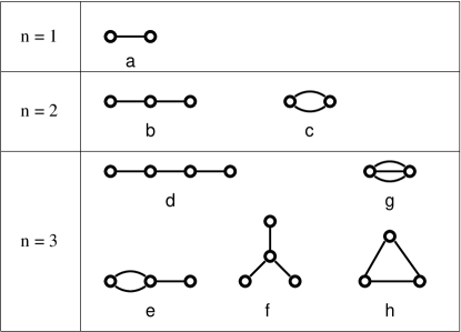
Figure 1: Diagrams contributing to the expansion of the grand canonical potential in terms of generalized “hopping” matrix elements (full lines) and bare cumulants (small circles). The contributions from diagrams a, b, d, e, f, and g are non-zero only if $H_{1}$ contains terms with bosonic X-operators having non-zero average values (Q-operators).

Our next task is to write an expansion for the Green’s functions of the Hubbard operators. We define

$$\bar{G}_{\alpha\beta~{}\alpha^{\prime}\beta^{\prime}}(i,j;\tau,\tau^{\prime})=-Tr\{\hat{\rho}~{}\hat{T}[X_{i}^{\alpha\beta}(\tau)X_{j}^{\alpha\beta}(\tau^{\prime})]\},$$ (16)

where the statistical operator $\hat{\rho}$ is given by Eq. (8), and the Hubbard operators are in the Heisenberg representation,

$$X_{i}^{\alpha\beta}(\tau)=e^{H\tau}X_{i}^{\alpha\beta}e^{-H\tau}.$$ (17)

The perturbation expansion for the Green’s functions is similar to the expansion for the grand-canonical potential. The consequence of the presence of two extra X-operators in (16) is that the corresponding diagrams will be rooted, i.e. one (for $i=j$) or two of the vertices will have fixed site indices and some fixed single-site state indices. The general rules are analogous to those for the Hubbard modelmetz , with the difference that extra indices (associated with the single-site states) are carried by the “hopping” matrix elements and the bare cumulants. A special case occurs when bosonic X-operators with non-zero average values, $\langle X^{\alpha\beta}\rangle=Q^{\alpha\beta}$, which we will call Q-operators, are present in $H_{1}$. In this case, as mentioned before, cumulants of order n with n odd may be non-zero, leading to disconnected rooted diagrams in the expansion of $\bar{G}_{\alpha\beta\alpha^{\prime}\beta^{\prime}}$. By simply regrouping the contributions from disconnected diagrams we can write:

$$\bar{G}_{\alpha\beta~{}\alpha^{\prime}\beta^{\prime}}(i,j;\tau,\tau^{\prime})=G_{\alpha\beta~{}\alpha^{\prime}\beta^{\prime}}(i,j;\tau,\tau^{\prime})-\langle X_{i}^{\alpha\beta}\rangle\langle X_{i}^{\alpha^{\prime}\beta^{\prime}}\rangle,$$ (18)

where $\langle X_{i}^{\alpha\beta}\rangle$ represents the average of the operator $X_{i}^{\alpha\beta}$ with respect to the full Hamiltonian, and $G_{\alpha\beta\alpha^{\prime}\beta^{\prime}}$ has a diagrammatic representation containing only connected diagrams. In the rest of this work we will always use the “connected” Green’s functions defined by (18). Obviously, if $H_{1}$ does not contain Q-operators, $G$ and $\bar{G}$ coincide, as the averages in (18) vanish. To summarize, we present in Fig. 2 some leading contributions to $G$.

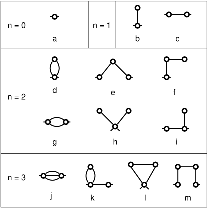
Figure 2: Diagrams representing the leading contributions to the expansion of the Green’s function around the atomic limit. The cumulants characterized by fixed site and state labels have small legs attached to the corresponding circle. For $n=3$ only diagrams containing cumulants with an even number of legs are shown.

At this point, a brief discussion about the Fourier transformation of the Green’s functions and of the cumulants is required. Due to the fact that the Hubbard operators have either bosonic-like or fermionic-like characters, the Fourier transformed Green’s functions, $G_{\alpha\beta~{}\alpha^{\prime}\beta^{\prime}}(i,j;i\omega_{n})$, will have odd Matsubara frequency, if both X-operators are fermionic, or even Matsubara frequency otherwise. On the other hand, the cumulants may depend on both even and odd Matsubara frequencies. Recalling the definition, Eqs. (14-15), a pair of indices $\alpha_{k}\beta_{k}$ associated with a fermionic-like Hubbard operator will induce a dependence on an odd frequency $\omega_{k}$, while an even frequency will be associated with a pair with bosonic character. A line connecting two vertices, and yielding the factor $E_{ij}^{\alpha\beta~{}\alpha^{\prime}\beta^{\prime}}$, will carry the frequency corresponding to the nature of the two pairs $(\alpha\beta)$ and $(\alpha^{\prime}\beta^{\prime})$. This nature is always the same as a result of the fact that the Hamiltonian conserves the number of particles. In the rest of this work we will not use different notations for odd and even frequencies, but we should keep in mind this aspect of the problem.

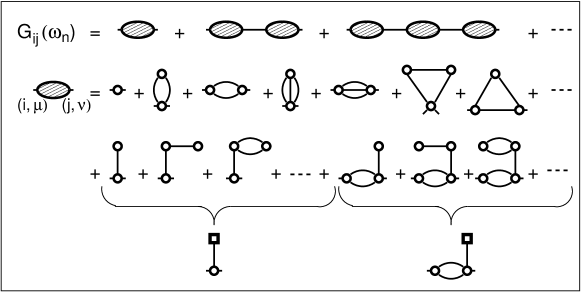
Figure 3: Diagrammatic representation of the renormalized expansion of the Green’s function and some leading contributions to the irreducible two-point cumulant $M_{ij}^{\mu\nu}(i\omega_{n})$. The simplified notation $(\alpha\beta)=\mu$, $(\alpha^{\prime}\beta^{\prime})=\nu$ was used. The diagrams containing one-particle reducible decorations of bare cumulants can be summed and replaced by diagrams with decorations equal to $\sum_{j,\nu}E_{ij}^{\mu~{}\nu}\langle X_{j}^{\nu}\rangle$. The average $\langle X_{j}^{\nu}\rangle$ is represented diagrammatically by a square.

The expansion that we derived is rather complicated and it may be of little help if used directly. However, we know that in order to obtain self-consistent approximations and, in particular, DMFT-type equations, a renormalized expansion is necessary. The key in obtaining a renormalized expansion is to introduce the notion of irreducibility with respect to one line (representing $E_{ij}^{\alpha\beta~{}\alpha^{\prime}\beta^{\prime}}$). We define the irreducible two-point cumulant, $M_{ij}^{\alpha\beta~{}\alpha^{\prime}\beta^{\prime}}(i\omega_{n})$, as the sum of all connected diagrams having two external legs (labeled by $\alpha\beta$ and $\alpha^{\prime}\beta^{\prime}$, respectively), with the property that the two legs cannot be separated by cutting one line. This definition differs slightly from the standard definitionmetz ; review , which requires that the diagram be not disconnected by cutting a single line. The difference comes from the existence of cumulants with odd number of legs. If $H_{1}$ does not contain Q-operators, the standard diagrammatics, along with the usual definition of irreducibility are valid. Some typical, low order contributions to the irreducible cumulant $M_{ij}^{\alpha\beta~{}\alpha^{\prime}\beta^{\prime}}(i\omega_{n})$ are shown in Fig.3. Notice that we can classify the diagrams into classes, each class containing one “basic” diagram that is one-particle irreducible with respect to all “hopping” lines plus diagrams derived from it by decorating the bare cumulants with reducible contributions. It is useful to perform partial summations of the diagrams in each class. The resulting diagrams will have all the reducible decorations replaced by factors equal to $\sum_{j,\alpha^{\prime},\beta^{\prime}}E_{ij}^{\alpha\beta~{}\alpha^{\prime}\beta^{\prime}}\langle X_{j}^{\alpha^{\prime}\beta^{\prime}}\rangle$.

We can now write a renormalized expansion for the Green’s functions in terms of irreducible cumulants and “hopping” matrix elements. The diagrammatic representation of this expansion is shown in Fig.3. Analytically, the corresponding equation will be:

$$G_{ij}^{\mu\nu}=M_{ij}^{\mu\nu}+\sum_{k,l}\sum_{\rho,\pi}~{}M_{ik}^{\mu\rho}E_{kl}^{\rho\pi}G_{lj}^{\pi\nu},$$ (19)

where, to reduce the number of indices, we introduced a simplified notation for a pair of single-site states, $(\alpha\beta)=\mu$. It is also convenient to regard a quantity $A^{\mu\nu}$ as an element of a matrix $\mathbf{A}$. Using this matrix notation, and Fourier transforming the spatial dependence, one can write the relation between the irreducible cumulant and the X-operator Green’s function,

$$\mathbf{G}(\mathbf{k},i\omega_{n})=\left[\mathbf{M}^{-1}(\mathbf{k},i\omega_{n})-\mathbf{E}(\mathbf{k})\right]^{-1},$$ (20)

where $\mathbf{E}(\mathbf{k})$ is the Fourier transform of the coupling constant matrix. What exactly are the Green’s function included in the matrix $\mathbf{G}$? Obviously, those that are coupled by the generalized “hopping” $E_{ij}^{\mu\nu}$. Specifically, if $\{\mu_{n}\}_{n={1,...,P}}$ and $\{\nu_{n}\}_{n={1,...,P}}$ are the sets of single-site pairs that label the coupling constants in $H_{1}$, each pair appearing only once in the corresponding set, the matrices will have dimension P and the matrix elements will be labeled $G^{\nu_{n}\mu_{n}}$, $M^{\nu_{n}\mu_{n}}$, and $E^{\mu_{n}\nu_{n}}$, respectively. A particular example of this construction will be presented in the next section for the Hubbard model.

Equations (19) and (20) represent the main result of this section. They are valid in arbitrary dimensions and for any Hamiltonian that has the form given by Eqs. (1-3) when written in terms of Hubbard operators.

III Generalized DMFT Equations

In the standard dynamical mean-field theoryreview , the single-particle self energy for the electron Green’s function is local in the limit of infinite spatial dimensions. However, for a general lattice Hamiltonian containing fermionic X-operators, this property is violated, as shown by Schillerschill in the case of correlated hopping. Nevertheless, one can overcome this problem by adopting a strong-coupling perspectiveshvaik and regarding the two-point irreducible cumulant, rather than the self-energy, as the the quantity in which the theory should be formulated. If $H_{1}$ contains only fermionic X-operators, and assuming that the coupling constants in $H_{1}$ are properly scaled, to keep the energy (per site) finite, one can showmetz ; review that the irreducible cumulants become local,

$$\mathbf{M}_{ij}(i\omega_{n})=\delta_{ij}\mathbf{M}_{0}(i\omega_{n}).$$ (21)

Consequently, the natural quantity in which such a theory should be formulated is the irreducible cumulant, rather than the self-energy. This becomes immediately transparent using Eqs. (20) and (21), and the fact that the electron Green’s function is given by the sum

$$\mathcal{G}_{\sigma}(\mathbf{k},i\omega_{n})=G^{0\sigma~{}\sigma 0}(\mathbf{k},i\omega_{n})+G^{\bar{\sigma}2~{}2\bar{\sigma}}(\mathbf{k},i\omega_{n})+\sigma[G^{0\sigma~{}2\bar{\sigma}}(\mathbf{k},i\omega_{n})+G^{\bar{\sigma}2~{}\sigma 0}(\mathbf{k},i\omega_{n})].$$ (22)

Although $\mathbf{M}_{0}$ is k-independent, $\mathcal{G}$ will have, in general, a complicated dependence on the wave-number, and the corresponding self-energy will be non-local, breaking the standard DMFT scheme. Formally, a self-energy matrix can be introduced by defining

$$\mathbf{\Sigma}(z)=(z+\mu)\mathbf{I}-\mathbf{E}-\mathbf{G}^{-1}(z)=(z+\mu)\mathbf{I}-\mathbf{M}_{0}^{-1}(z),$$ (23)

with $\mathbf{I}$ being the identity matrix. However, in general, this quantity does not have the desired analytic propertiesshvaik and may diverge as $|z|\rightarrow\infty$.

If we go further and generalize the model to include both fermionic and bosonic degrees of freedom, the picture presented above fails, as one cannot scale the coupling constants in such a way that one has both finite energy (per site) and local irreducible cumulants in the limit of infinite dimensionspkm . In contrast, this work assumes a different perspective: rather than viewing DMFT as an approximation that becomes exact in the limit of infinite coordination, we see it as the first order approximation in a hierarchy of (increasing size) cluster approximations. In this picture, the exact limit is obtained for an infinite-large cluster. Consequently, our G-DMFT scheme will be defined by the condition that the two-point irreducible cumulant be local. Unlike the case of extended DMFT, we have no small parameter (other than the inverse of the cluster size) justifying this approach. Obviously, if the model contains only fermionic degrees of freedom, the two perspectives described above are equivalent.

Based on the locality of $\mathbf{M}$, we can approach the central step in a DMFT-type scheme, namely the self-consistent mapping of the lattice problem onto an effective impurity problem. Let us consider the single-impurity problem with the statistical operator

$$\hat{\rho}_{imp}=e^{-\beta H_{0}^{imp}}\hat{T}\exp\left\{-\int_{0}^{\beta}d\tau\left[\int_{0}^{\beta}d\tau^{\prime}~{}\sum_{\alpha\beta~{}\alpha^{\prime}\beta^{\prime}}X^{\alpha\beta}(\tau)\Delta^{\alpha\beta~{}\alpha^{\prime}\beta^{\prime}}(\tau-\tau^{\prime})X^{\alpha^{\prime}\beta^{\prime}}(\tau^{\prime})+\sum_{\alpha,\beta\in\mathcal{B}_{Q}}h_{imp}^{\alpha\beta}(\tau)X^{\alpha\beta}(\tau)\right]\right\},$$ (24)

where $h_{imp}(\tau)$ is an external field that couples to the Q-operators, $\mathcal{B}_{Q}$ is the set of indices corresponding to the Q-operators, $\mathbf{\Delta}(\tau-\tau^{\prime})$ is the hybridization matrix and $H_{0}^{imp}$ contains one term, for example $i=0$, from the local Hamiltonian (2). Using the expansion procedures described in the previous section, with the hybridization replacing the “hopping” matrix $\mathbf{E}$, we obtain for the impurity Green’s function a relation similar to (20),

$$\mathbf{G}_{imp}(i\omega_{n})=\left[\mathbf{M}_{imp}^{-1}(i\omega_{n})-\mathbf{\Delta}(i\omega_{n})\right]^{-1},$$ (25)

where all the quantities are local, and $\mathbf{M}_{imp}$ is the irreducible cumulant with respect to the hybridization. For practical calculations, as well as to gain some physical insight, it is useful to express the impurity problem in a Hamiltonian form. Taking into account that in our matrix formulation the indices $(\alpha\beta)$ corresponding to fermionic and bosonic Hubbard operators do not mix, all the matrices, including $\Delta^{\alpha\beta~{}\alpha^{\prime}\beta^{\prime}}$, are block-diagonal with one block corresponding to the fermionic indices and one to the bosonic sector. Consequently, we will introduce two types of auxiliary degrees of freedom, one associated with a fermionic bath, described by operators $(a_{k\sigma},a_{k\sigma}^{\dagger})$, and one associated with a bosonic bath, described by $(b_{k\sigma},b_{k\sigma}^{\dagger})$. The impurity Hamiltonian will be

$$H_{imp} = H_{0}^{imp}+\sum_{(\alpha\beta)\in\mathcal{B}_{Q}}h_{imp}^{\alpha\beta}X^{\alpha\beta}+\sum_{k,\sigma}\epsilon_{k}^{a}a_{k\sigma}^{\dagger}a_{k\sigma}+\sum_{k,\sigma}\epsilon_{k}^{b}b_{k\sigma}^{\dagger}b_{k\sigma}$$ (26)

$$+ \sum_{k}\sum_{(\alpha\beta)\in\mathcal{F}}[V_{a}^{\alpha\beta}(k)~{}a_{k\sigma_{\alpha\beta}}^{\dagger}X^{\alpha\beta}+h.c.]+\sum_{k}\sum_{(\alpha\beta)\in\mathcal{B}}[V_{b}^{\alpha\beta}(k)~{}b_{k\sigma_{\alpha\beta}}^{\dagger}X^{\alpha\beta}+h.c.].$$

The first term in the right hand side describes an isolated impurity, the second term represents the coupling to the external field and the summation is restricted to labels corresponding to bosonic operators having a non-zero mean value, the Q-operators ($\mathcal{B}_{Q}$), the third and forth terms describe the fermionic and bosonic baths, respectively, and the last two terms represent the coupling of the impurity with the two baths. In the last two terms, the summations over the X-operator labels $(\alpha\beta)$ are restricted to the fermionic ($\mathcal{F}$) and bosonic sectors ($\mathcal{B}$), respectively. The expression of the hybridization in terms of coupling constants $V^{\alpha\beta}(k)$ can be obtained by integrating out the auxiliary degrees of freedom. We have

$$\Delta^{\alpha\beta~{}\alpha^{\prime}\beta^{\prime}}(i\omega_{n})=\frac{1}{N}\sum_{k}\frac{V_{l}^{\alpha\beta}(k)V_{l}^{\alpha^{\prime}\beta^{\prime}}(k)}{i\omega_{n}-\epsilon_{k}^{l}},$$ (27)

where $l=a$ if the element is in the fermionic sector of the $\Delta$ matrix and $l=b$ for the bosonic case.

Returning to our main problem, we obtain the self-consistency conditions by requiring that the lattice irreducible cumulant be equal to the effective impurity problem irreducible cumulant, $\mathbf{M}_{imp}(z)=\mathbf{M}_{0}(z)$. By comparing the diagrammatic expansion of $\mathbf{M}_{imp}$ in terms of bare cumulants (dressed with external field lines) and hybridization functions with the expansion of $\mathbf{M}_{0}$, we observe that the equality is satisfied if we identify a line representing $\Delta^{\mu\nu}$ with the sum of all the paths starting with $E_{0i}^{\mu\rho}$ and ending with $E_{j0}^{\pi\nu}$, as well as the sum betweeen an external field line $h^{\mu}$ and the one-particle reducible decoration $\sum_{\nu}\Delta^{\mu\nu}\langle X^{\nu}\rangle$ with the lattice one-particle reducible decoration $\sum_{j,\nu}E_{ij}^{\mu~{}\nu}\langle X_{j}^{\nu}\rangle$. Explicitly, the expansion for the impurity irreducible cumulant is identical with the expansion of the lattice irreducible cumulant provided

$$\mathbf{\Delta}(i\omega_{n})=\sum_{i,j}~{}\mathbf{E}_{0i}\mathbf{G}_{ij}^{(0)}(i\omega_{n})\mathbf{E}_{j0},$$ (28)

where $\mathbf{G}_{ij}^{(0)}(i\omega_{n})$ represents the matrix Green’s function for a lattice with the site “0” removed, together with a condition that determines self-consistently the external field $h$,

$$h_{imp}^{\mu}=\sum_{j,~{}\nu\in\mathcal{B}_{Q}}E_{0j}^{\mu\nu}\langle X_{j}^{\nu}\rangle-\sum_{\nu}\Delta^{\mu\nu}(0)\langle X_{0}^{\nu}\rangle.$$ (29)

Notice that equation (28) represents the generalization of the well known DMFT self-consistency conditionreview . In addition, if the non-local Hamiltonian $H_{1}$ contains Hubbard operators that acquire a non-zero mean value, our lattice model is mapped into an impurity model with an external field determined self-consistently by equation (29).

Our final step consists in finding a self-consistent equation that determines the hybridization $\Delta(z)$ in terms of the lattice Green’s function. Comparing Eq. (19) for $\mathbf{G}_{ij}$ (after making $\mathbf{M}_{ij}=\delta_{ij}\mathbf{M}_{0}$) with the equivalent expression for $\mathbf{G}_{ij}^{(0)}$,

$$\mathbf{G}_{ij}^{(0)}(i\omega_{n})=\delta_{ij}\mathbf{M}_{0}(i\omega_{n})+\sum_{k\neq 0}\mathbf{M}_{0}(i\omega_{n})\mathbf{E}_{ik}\mathbf{G}_{kj}^{(0)}(i\omega_{n})~{}~{}~{}~{}~{}~{}~{}~{}~{}\mbox{for}~{}~{}i,j\neq 0,$$ (30)

we obtain for $i=j=0$:

$$\mathbf{G}_{00}(i\omega_{n}) = \mathbf{M}_{0}(i\omega_{n})+\mathbf{M}_{0}(i\omega_{n})\sum_{k,l}~{}\mathbf{E}_{0k}\mathbf{G}_{kl}^{(0)}(i\omega_{n})\mathbf{E}_{l0}~{}\mathbf{M}_{0}(i\omega_{n})+~{}.~{}.~{}.$$ (31)

$$= \mathbf{M}_{0}\left[\mathbf{1}-\sum_{k,l}~{}\mathbf{E}_{0k}\mathbf{G}_{kl}^{(0)}(i\omega_{n})\mathbf{E}_{l0}~{}\mathbf{M}_{0}(i\omega_{n})\right]^{-1}.$$

Using equation (28) for $\mathbf{\Delta}(i\omega_{n})$ and the Fourier transform for the local Green’s function, we obtain the self-consistent condition that determines the hybridization,

$$\frac{1}{N}\sum\left[\mathbf{M}_{0}^{-1}(i\omega_{n})-\mathbf{E}(\mathbf{k})\right]^{-1}=\left[\mathbf{M}_{0}^{-1}(i\omega_{n})-\mathbf{\Delta}(i\omega_{n})\right]^{-1}.$$ (32)

Formally, Eq. (32) closely resembles the standard form of the DMFT self-consistency conditionreview . We should, however, keep in mind the fact that this is a matrix equation involving Green’s functions for the Hubbard operators. To solve a problem described by the Hamiltonian (1-3) within this scheme, implies to solve the impurity problem, (24), find an irreducible cumulant matrix $\mathbf{M}_{0}$, then use the self-consistency condition (32) together with equation (29) to determine the new hybridization, $\mathbf{\Delta}(i\omega_{n})$, and the new field $\mathbf{h}_{imp}$. The process is repeated until convergence is reached.

III.1 The Hubbard Model

In order to get a feeling of how this approach works, as well as to check its validity, we can do a simple exercise by applying the procedure to the Hubbard model, for which we should be able to recover the known DMFT results. In this particular case, the Hamiltonian will be

$$H_{HUB}=\sum_{i}[-\mu(X_{i}^{\uparrow\uparrow}+X_{i}^{\downarrow\downarrow})+(U-2\mu)X_{i}^{22}]+\sum_{i,j}\sum_{\sigma}~{}t_{ij}[X_{i}^{\sigma 0}X_{j}^{0\sigma}+X_{i}^{2\bar{\sigma}}X_{j}^{\bar{\sigma}2}+\sigma X_{i}^{\sigma 0}X_{j}^{\bar{\sigma}2}+\sigma X_{i}^{2\bar{\sigma}}X_{j}^{0\sigma}],$$ (33)

where $\mu$ represents the chemical potential, $U$ the on-site Coulomb interaction and $t_{ij}$ the hopping matrix elements, which are equal to $-t$ if i and j are nearest neighbors and zero otherwise. We can introduce the hopping matrix,

$$\mathbf{E}(\mathbf{k})=\left(\begin{array}[]{cc}E^{\sigma 0~{}0\sigma}(\mathbf{k})&E^{\sigma 0~{}\bar{\sigma}2}(\mathbf{k})\\ E^{2\bar{\sigma}~{}0\sigma}(\mathbf{k})&E^{2\bar{\sigma}~{}\bar{\sigma}2}(\mathbf{k})\\ &\end{array}\right)=\left(\begin{array}[]{cc}\epsilon_{k}&\sigma\epsilon_{k}\\ \sigma\epsilon_{k}&\epsilon_{k}\\ &\end{array}\right),$$ (34)

where $\epsilon_{k}$ is the Fourier transform of $t_{ij}$. Next, we introduce the Green’s function matrix and the irreducible cumulant matrix:

$$\mathbf{G}=\left(\begin{array}[]{cc}G^{0\sigma~{}\sigma 0}&G^{0\sigma~{}2\bar{\sigma}}\\ G^{\bar{\sigma}2~{}\sigma 0}&G^{\bar{\sigma}2~{}2\bar{\sigma}}\\ &\end{array}\right);~{}~{}~{}~{}~{}~{}~{}~{}~{}~{}\mathbf{M}=\left(\begin{array}[]{cc}M^{0\sigma~{}\sigma 0}&M^{0\sigma~{}2\bar{\sigma}}\\ M^{\bar{\sigma}2~{}\sigma 0}&M^{\bar{\sigma}2~{}2\bar{\sigma}}\\ &\end{array}\right).$$ (35)

Our goal is to show that the matrix equation (32) reduces in this particular case to the well known DMFT self-consistency condition,

$$\mathcal{G}_{0}^{-1}(i\omega_{n})=i\omega_{n}+\mu-\Delta_{0}(i\omega_{n})=\left[\frac{1}{N}\sum_{\mathbf{k}}\frac{1}{i\omega_{n}+\mu-\epsilon_{k}-\Sigma(i\omega_{n})}\right]^{-1}+\Sigma(i\omega_{n}),$$ (36)

where $\Sigma(i\omega_{n})$ represents the self-energy of the single-particle electron Green’s function and $\Delta_{0}(i\omega_{n})$ the hybridization of the effective single-impurity problem. The electron single-particle Green’s function, $\mathcal{G}$, is given by a sum of all the elements of $\mathbf{G}$, as shown in Eq. (22). Similarly, we define the quantity

$$\mathcal{M}(i\omega_{n})=M^{0\sigma~{}\sigma 0}(i\omega_{n})+M^{\bar{\sigma}2~{}2\bar{\sigma}}(i\omega_{n})+\sigma[M^{0\sigma~{}2\bar{\sigma}}(i\omega_{n})+M^{\bar{\sigma}2~{}\sigma 0}(i\omega_{n})].$$ (37)

It is straightforward to show that the matrix Green’s function has the structure:

$$\mathbf{G}(\mathbf{k},i\omega_{n})=[\mathbf{M}^{-1}(i\omega_{n})-\mathbf{E}(\mathbf{k})]^{-1}=\frac{1}{1-\epsilon_{k}\mathcal{M}(i\omega_{n})}\mathbf{M}(i\omega_{n})+\delta\frac{\epsilon_{k}}{1-\epsilon_{k}\mathcal{M}(i\omega_{n})}\left(\begin{array}[]{cc}-1&\sigma\\ \sigma&-1\\ &\end{array}\right),$$ (38)

where $\delta=\det\{\mathbf{M}\}$. Using Eq. (38) and the expression (22) for the electron Green’s function, together with the definition of $\mathcal{M}$, we have

$$\mathcal{G}(\mathbf{k},i\omega_{n})=\frac{1}{\mathcal{M}^{-1}(i\omega_{n})-\epsilon_{k}},$$ (39)

which shows that $\mathcal{M}(i\omega_{n})$ is the single particle irreducible cumulant, $\mathcal{M}^{-1}(i\omega_{n})=i\omega_{n}+\mu-\Sigma(i\omega_{n})$, where $\Sigma(i\omega_{n})$ is the single particle self-energy. On the other hand, making the summation over $k$ in Eq. (38) and introducing the result in the self-consistency relation (32) gives:

$$\mathbf{\Delta}=\Delta_{0}\left(\begin{array}[]{cc}1&\sigma\\ \sigma&1\\ &\end{array}\right),$$ (40)

with

$$\Delta_{0}=\frac{b}{a\delta},~{}~{}~{}~{}~{}~{}~{}~{}~{}a=\frac{1}{n}\sum_{\mathbf{k}}\frac{1}{1-\epsilon_{k}\mathcal{M}},~{}~{}~{}~{}~{}~{}~{}~{}~{}b=\frac{\delta(a-1)}{\mathcal{M}}.$$ (41)

Taking into account the structure of $\mathbf{\Delta}$ given by Eq. (40), the impurity problem described by the statistical operator (24) reduces to an Anderson single impurity problem with a hybridization $\Delta_{0}$. Finally, we have

$$\Delta_{0}(i\omega_{n})=\mathcal{M}^{-1}(i\omega_{n})-\left[\frac{1}{N}\sum_{\mathbf{k}}\frac{1}{\mathcal{M}^{-1}(i\omega_{n})-\epsilon_{k}}\right]^{-1},$$ (42)

which represents the standard DMFT self-consistency equation.

IV A Functional Approach

Functionals of Green’s functions provide an elegant and powerful tool for formulating dynamical mean-field theories. Within this framework, the DMFT equations are obtained as a direct result of a simple approximation on the Baym-Kadanoff functionalreview . The extended dynamical mean-field equations have also been rigorously derived using a functional techniqueedmft5 . Moreover, the functional perspective seems to offer the natural framework for cluster generalizations of the dynamical mean-field theory that include effects of short-range correlations. The purpose of this section is to introduce a strong-coupling generalization of the functional DMFT formulationshvaik . The construction of a generalized Baym-Kadanoff-type functional will allow us to present an alternative derivation of the generalized DMFT equations, and, more importantly, will set the basis for a future cluster extension of the G-DMFT approach.

The main idea of the functional interpretation of DMFT is to formulate a local approximation for the Baym-Kadanoff functional $\Phi[G]$, which is the sum of all vacuum-to-vacuum skeleton (two-particle irreducible) diagrams constructed with the full propagator $G$ and the interaction vertices. This functional has the property that

$$\Sigma_{ij}(i\omega_{n})=\frac{\delta\Phi}{\delta G_{ji}(i\omega_{n})}~{}~{},$$ (43)

where $\Sigma_{ij}(i\omega_{n})$ is the self-energy. As the coordination number of the lattice goes to infinity, the self-energy becomes local and $\Phi$ will depend only on the local Green’s functions, $G_{ii}$:

$$\Phi=\sum_{i}~{}\phi[G_{ii}],$$ (44)

where $\phi[G_{ii}]$ is a functional of the local Green’s function at site $i$ only. This scheme cannot be transfered directly to approach our strong-coupling problem. As we mentioned above, within our strong-coupling perspective, the natural quantity to describe the system is the two-point irreducible cumulant, $M_{ij}(i\omega_{n})$, rather than the self-energy. Our task is to identify a conjugate quantity (which cannot be the Green’s, function but rather something with dimensions of energy), and to construct a functional of this quantity that will determine $M$ by a relation similar to (43).

Following Refs. shvaik, and shvaik1, , we start by introducing two time dependent external sources, one , $J_{ij}^{\mu\nu}(\tau-\tau^{\prime})$, coupled to the X-operator Green’s functions, and the other, $\lambda_{i}^{\alpha\beta}(\tau)$, coupled to the average $Q_{i}^{\alpha\beta}=\langle X_{i}^{\alpha\beta}\rangle$ of the bosonic Hubbard operators that occur in the non-local Hamiltonian $H_{1}$. The corresponding generating functional will be

$$\Omega[J,\lambda]=-\frac{1}{\beta}\ln Tr\hat{\rho}[J,\lambda],$$ (45)

where the statistical operator $\rho$ is given by

$$\hat{\rho}[J,\lambda]=e^{-\beta H_{0}}\hat{T}\exp\left\{-\int_{0}^{\beta}d\tau\left[\int_{0}^{\beta}d\tau^{\prime}\left(H_{1}(\tau,\tau^{\prime})+\sum_{i,j}\sum_{\mu,\nu}J_{ji}^{\nu\mu}(\tau-\tau^{\prime})X_{i}^{\mu}(\tau)X_{j}^{\nu}(\tau^{\prime})\right)+\sum_{i,\mu}\lambda_{i}^{\mu}(\tau)X_{i}^{\mu}(\tau)\right]\right\}.$$ (46)

The field $J_{ij}^{\mu\nu}(\tau-\tau^{\prime})$ is equivalent with introducing frequency dependent coupling constants $E_{ji}^{\nu\mu}(i\omega_{n})=E_{ji}^{\nu\mu}+J_{ji}^{\nu\mu}(i\omega_{n})$. The Green’s functions can be expressed as functional derivatives of the generating functional, $\Omega[J,\lambda]$, with respect to the frequency dependent field,

$$G_{ij}^{\mu\nu}(i\omega_{n})-\beta\langle X_{i}^{\mu}\rangle\langle X_{j}^{\nu}\rangle=-\beta\frac{\delta\Omega[J,\lambda]}{\delta E_{ji}^{\nu\mu}(i\omega_{n})}\Bigg{|}_{J=0,\lambda=0},$$ (47)

where the average value $Q_{i}^{\mu}=\langle X_{i}^{\mu}\rangle$ is non-zero only if $X_{i}^{\mu}$ is a Q-operator. The generating functional $\Omega[J,\lambda]$ reduces to the grand-canonical potential, $\Omega$, in the absence of the external sources.

The next step is to integrate Eq. (47). As we are interested in a strong-coupling equivalent of the Baym-Kadanoff functional, we will express the Green’s function in terms of the two-point irreducible cumulant, rather than the self-energyshvaik . Using the notation $\hat{\mathbf{A}}$ for a tensor with elements $A_{ij}^{\mu\nu}$, we can formally write equation (19) as

$$\hat{\mathbf{G}}=\left[\hat{\mathbf{I}}-\hat{\mathbf{M}}\hat{\mathbf{E}}\right]^{-1}\hat{\mathbf{M}},$$ (48)

where $\hat{\mathbf{I}}$ is the identity tensor, $I_{ij}^{\mu\nu}=\delta_{ij}\delta_{\mu\nu}$. By integrating (47) with $\hat{\mathbf{G}}$ given by (48) we obtain

$$\Omega[J,\lambda]=\Omega_{0}+\frac{1}{\beta}\sum_{\omega_{n}}Tr~{}\ln[\hat{\mathbf{I}}-\hat{\mathbf{M}}\hat{\mathbf{E}}]+\frac{1}{\beta}\sum_{\omega_{n}}Tr[\hat{\mathbf{M}}\hat{\mathbf{{\mathcal{E}}}}]+\Xi[J,\lambda],$$ (49)

with $\Omega_{0}$ the grand-canonical potential in the atomic limit. The quantity $\hat{\mathbf{{\mathcal{E}}}}$ is the renormalized coupling constant (or renormalized generalized hopping) and can be represented diagrammatically as a sum of chains of “hopping” lines and irreducible cumulants. Analytically we have

$${\mathcal{E}}_{ij}^{\mu\nu}=E_{ij}^{\mu\nu}+\sum_{p,q}\sum_{\alpha,\beta}~{}E_{iq}^{\mu\alpha}M_{qp}^{\alpha\beta}E_{pj}^{\beta\nu}+.~{}.~{}.=\left[\hat{\mathbf{E}}(\hat{\mathbf{I}}-\hat{\mathbf{M}}\hat{\mathbf{E}})^{-1}\right]_{ij}^{\mu\nu}.$$ (50)

The last term in Eq. (49) is a functional with the property

$$-\beta\frac{\delta\Xi[J,\lambda]}{\delta E_{ji}^{\nu\mu}(i\omega_{n})}=Tr\left[\hat{\mathbf{M}}\frac{\delta\hat{\mathbf{{\mathcal{E}}}}}{\delta E_{ji}^{\nu\mu}(i\omega_{n})}\right]-\beta\langle X_{i}^{\mu}\rangle\langle X_{j}^{\nu}\rangle.$$ (51)

Also, because the functional derivative of $\Omega[J,\lambda]$ with respect to $\lambda$ gives the average value of $X_{i}^{\mu}$, we will have

$$\frac{\delta\Xi}{\delta\lambda_{i}^{\mu}}=-\frac{1}{\beta}Tr\left[\hat{\mathbf{M}}\frac{\delta\hat{\mathbf{{\mathcal{E}}}}}{\delta\lambda_{i}^{\mu}}\right]+\langle X_{i}^{\mu}\rangle.$$ (52)

The standard way to proceed is to perform a Legendre transform of the generating functional with respect to the interacting single-particle Green’s function and to eliminate the external source $J$ in favor of $G$ in the functionals. Instead, by analyzing equations (51) and (52), we identify the renormalized coupling constant ${\mathcal{E}}_{ij}^{\mu\nu}$ as the quantity conjugate with the irreducible cumulant and use it as an independent variable. Consequently, we introduce the new functionals $\Omega^{*}[{\mathcal{E}},\lambda;E]$ and $\Xi^{*}[{\mathcal{E}},\lambda;E]$, with

$$\Omega^{*}[{\mathcal{E}}[J,\lambda],\lambda;E+J]=\Omega[J,\lambda],~{}~{}~{}~{}~{}~{}~{}~{}~{}~{}~{}~{}\Xi^{*}[{\mathcal{E}}[J,\lambda],\lambda;E+J]=\Xi[J,\lambda].$$ (53)

The dependence on the last variable, $E$, involves only the components of the coupling constant tensor corresponding to Q-operator indices and we have

$$\frac{\delta\Xi^{*}}{\delta E_{ij}^{\mu~{}\nu}}=\langle X_{i}^{\mu}\rangle\langle X_{j}^{\nu}\rangle.$$ (54)

The functional derivative with respect to $\lambda$ of both $\Omega^{*}$ and $\Xi^{*}$ will give the average value of the bosonic X operator, while for the Luttinger-Ward-type functional $\Xi^{*}$ we have

$$-\beta\frac{\delta\Xi^{*}}{\delta{\mathcal{E}}_{ji}^{\nu\mu}(i\omega_{n})}=M_{ij}^{\mu\nu}(i\omega_{n}).$$ (55)

This equation is the strong-coupling equivalent of (43) and determines the irreducible two-point cumulant as a functional of the renormalized “hopping” matrix, the bare diagonal coupling elements and the external fields. The stationarity condition $\delta\Omega^{*}/\delta{\mathcal{E}}_{ji}^{\nu\mu}=0$ yields the relation between the renormalized couplings and the cumulants, ${\mathcal{E}}_{ij}^{\mu\nu}=[\hat{\mathbf{E}}(\hat{\mathbf{I}}-\hat{\mathbf{M}}\hat{\mathbf{E}})^{-1}]_{ij}^{\mu\nu}$, which is identical to the definition (50). Again, at stationarity and in the absence of the external fields the functional $\Omega^{*}$ reduces to the grand canonical potential.

For the case with no Q-operators in the non-local Hamiltonian our construction is complete. In this particular case the only relevant dependence in the functionals is on the renormalized coupling ${\mathcal{E}}$. The functional $\Omega^{*}[{\mathcal{E}}]$ is formally analogous to the functional $\Gamma_{new}[G]$ introduced by Chitra and Kotliaredmft5 from a weak-coupling perspective. In our picture the strong coupling correspondent of the self-energy is, as noted before, the irreducible cumulant, while the renormalized and bare coupling constants correspond to the full and non-interacting Green’s function, respectively. Also, the strong-coupling analog of the Luttinger-Ward functional $\Phi[G]$ is $\Xi^{*}[{\mathcal{E}}]$. Similarly to its weak-coupling counterpart, $\Xi^{*}[{\mathcal{E}}]$ can be expressed as a sum of all vacuum-to-vacuum skeleton diagrams containing bare cumulants and renormalized “hopping” lines. All the skeleton diagrams are two-particle irreducible, i.e. they cannot be separated into disconnected parts by cutting two ${\mathcal{E}}$ lines.

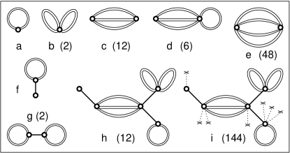
Figure 4: Generalized skeleton diagrams contributing to the functional $\Xi^{*}$. The contribution of the external field $\lambda$ is represented only in diagram (i) by dotted lines. The numbers in parentheses represent the symmetry factors (if different from 1) of the corresponding diagrams (the number of ways in which a graph can be made isomorphic with itself). The renormalized coupling ${\mathcal{E}}$ is represented by double lines.

In general, however, the diagrammatic expression of $\Xi^{*}$ is more complicated and involves, in addition to the bare cumulants, both renormalized coupling constants, ${\mathcal{E}}_{ji}^{\nu\mu}$, and bare coupling constants, $E_{ij}^{\mu\nu}$. Also, lines corresponding to the external field $\lambda$ have to be added. The generalized skeleton diagrams have to satisfy two conditions: i) Each diagram is two-particle irreducible with respect to the renormalized “hopping”; ii) By cutting any bare “hopping” line the diagram is divided into two disconnected parts. These conditions determine a tree-like structure for the generalized skeleton diagrams with skeleton blocks coupled by bare $E$ lines. This structure is illustrated in Fig. 4 for a few low-order contributions to $\Xi^{*}$. Due to the tree-like structure of the diagrams, it is rather difficult to find a local approximation for the functional $\Xi^{*}$. In order to overcome this problem, we proceed to the last step of our construction and define the Legendre transform of $\Omega^{*}$ with respect to the average of bosonic Hubbard operators, $Q_{i}^{\mu}=\langle X_{ij}^{\mu}\rangle$,

$$\Gamma[{\mathcal{E}},Q]=\Omega^{*}[{\mathcal{E}},\lambda;E]-\sum_{i}\sum_{\mu\in\mathcal{B}_{Q}}\lambda_{i}^{\mu}Q_{i}^{\mu},$$ (56)

where the bare coupling $E_{ij}^{\mu\nu}$ is treated as a parameter and is not written explicitly as an argument of the functional $\Gamma$. Using the condition $-\lambda_{i}^{\mu}=\delta\Gamma/\delta Q_{i}^{\mu}$ to eliminate $\lambda$, we obtain

$$\Gamma[{\mathcal{E}},Q]=\Omega_{0}+\frac{1}{\beta}\sum_{\omega_{n}}Tr~{}\ln[{\hat{\mathbf{I}}-\hat{\mathbf{M}}[{\mathcal{E}},Q]\hat{\mathbf{E}}}]+\frac{1}{\beta}\sum_{\omega_{n}}Tr[\hat{\mathbf{M}}[{\mathcal{E}},Q]\hat{\mathbf{{\mathcal{E}}}}]-\frac{1}{2}\sum_{i,j}\sum_{\mu,\nu\in\mathcal{B}_{Q}}Q_{i}^{\mu}E_{ij}^{\mu\nu}Q_{j}^{\nu}+\Psi[{\mathcal{E}},Q].$$ (57)

The properties with respect to ${\mathcal{E}}$ of the new functionals are similar to those of $\Omega^{*}$ and $\Xi^{*}$, namely the stationarity condition $\delta\Gamma/\delta{\mathcal{E}}_{ji}^{\nu\mu}=0$ yields equation (50), and we have

$$-\beta\frac{\delta\Psi[{\mathcal{E}},Q]}{\delta{\mathcal{E}}_{ji}^{\nu\mu}(i\omega_{n})}=M_{ij}^{\mu\nu}(i\omega_{n}).$$ (58)

In addition, stationarity with respect to $Q$, $\delta\Gamma/\delta Q_{i}^{\mu}=0$, yields

$$\frac{\delta\Psi[{\mathcal{E}},Q]}{\delta Q_{i}^{\mu}}=\sum_{j,~{}\beta\in\mathcal{B}_{Q}}E_{ij}^{\mu\nu}~{}Q_{j}^{\nu}.$$ (59)

The diagrammatic representation of the new Luttinger-Ward-type functional $\Psi$ contains skeleton diagrams that are two-particle irreducible with respect to the ${\mathcal{E}}$ lines and have cumulants dressed with $EQ$ contributions. The structure of the diagrams is illustrated in Fig 5. Using the diagrammatic representation of the functionals $\Psi$ and $\Xi^{*}$, as well as that of $Q$, and taking into account the symmetry factors associated with each diagram, it is straightforward to check that

$$\Psi[{\mathcal{E}},Q]=\Xi^{*}[{\mathcal{E}},\lambda=0;E]+\frac{1}{2}\sum_{i,j}\sum_{\mu,\nu\in\mathcal{B}_{Q}}Q_{i}^{\mu}E_{ij}^{\mu\nu}Q_{j}^{\nu},$$ (60)

where $Q_{i}^{\mu}=\langle X_{i}^{\mu}\rangle=\delta\Xi^{*}/\delta\lambda_{i}^{\mu}|_{\lambda=0}$.

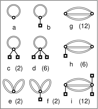
Figure 5: Example of diagrams contributing to $\Psi[{\mathcal{E}},Q]$. The average of a diagonal operator, $Q_{i}^{\alpha}$, is represented by a square. The symmetry factors are written in parentheses. If $Q_{i}^{\mu}=0$, the remaining basic skeleton diagrams (a, e, g, …) are identical with the remaining diagrams in Fig. 4 (a, b, c, …), and $\Psi=\Xi^{*}$. In general, we have the basic diagrams plus diagrams obtained by decorating the bare cumulants with lines and squares representing $E_{ij}^{\mu\nu}Q_{j}^{\nu}$.

We are prepared now to introduce the generalized DMFT from a functional perspective. By analogy with the standard approachreview , we construct an approximate theory by making the ansatz that the Luttinger-Ward functional $\Psi$ depends only on local renormalized “hopping” matrices, i.e.,

$$\Psi[{\mathcal{E}},Q]=\sum_{i}\psi[\mathbf{{\mathcal{E}}}_{ii},Q],$$ (61)

where $\psi$ is a functional that depends only on the local renormalized coupling constants at site i. In diagrammatic terms, it means that all the bare cumulants contained in a skeleton diagram contributing to $\psi$ are defined on the same site. A direct consequence of this ansatz is that the two-point irreducible cumulant of the theory is local,

$$\mathbf{M}_{ij}(i\omega_{n})=\frac{\delta\Psi}{\delta\mathbf{{\mathcal{E}}}_{ii}(i\omega_{n})}\delta_{ij},$$ (62)

with $\delta_{ij}$ being the Kronecker $\delta$ symbol. The stationarity condition for $\Gamma$ yields

$$\mathbf{{\mathcal{E}}}_{ii}=\left[\hat{\mathbf{E}}(\hat{\mathbf{I}}-\hat{\mathbf{M}}\hat{\mathbf{E}})^{-1}\right]_{ii}=\frac{1}{N}\sum_{k}\mathbf{E}(k)(\mathbf{I}-\mathbf{M}\mathbf{E}(k))^{-1},$$ (63)

where $M$ is given by (62) and, for the second equality, we assumed that the system is homogeneous. Relation (63) represents our generalized DMFT equation and it should be viewed as a functional equation for the local renormalized coupling matrix. To cast it in a more familiar form, let us observe that using the expressions for the Green’s function, Eq. (48), and for the renormalized coupling, Eq. (50), we have

$$\hat{\mathbf{G}}=\hat{\mathbf{M}}\hat{\mathbf{{\mathcal{E}}}}\hat{\mathbf{M}}+\hat{\mathbf{M}}.$$ (64)

Taking into account the local character of the irreducible cumulant, we obtain, for a homogeneous system,

$$\mathbf{G}_{ii}(i\omega_{n})=\frac{1}{N}\sum_{k}\left[\left(\frac{\delta\Psi}{\delta\mathbf{{\mathcal{E}}}_{ii}}\right)^{-1}-\mathbf{E}(k)\right]^{-1},$$ (65)

where $\mathbf{G}_{ii}(i\omega_{n})$ has to be understood as a functional of ${\mathcal{E}}$.

To be able to solve Eq. (63) or Eq. (65) we need to know the functional dependence of $\Psi$, at least approximately. A direct approach is rather hard in practice, therefore it is more convenient to generate the functionals from a purely local theory. A simple inspection of the diagrammatic expression for $\Psi$ (see Figure 5), shows that, in the case when all the bare cumulants are defined on the same site $i=0$, the same diagrams will correspond to an impurity problem defined by the statistical operator given by Eq. (24). In fact, taking into account the previous construction of the strong-coupling functionals, we have

$$\Gamma_{imp}[{\mathcal{D}},Q]=\frac{\Omega_{0}}{N} + \frac{1}{\beta}\sum_{\omega_{n}}Tr~{}\ln[{\mathbf{I}-\mathbf{M}_{imp}[{\mathcal{D}},Q]\mathbf{\Delta}}]+\frac{1}{\beta}\sum_{\omega_{n}}Tr[\mathbf{M}_{imp}[{\mathcal{D}},Q]\mathbf{{\mathcal{D}}}]$$

$$- \frac{1}{2}\sum_{\mu,\nu\in\mathcal{B}_{Q}}Q^{\mu}\Delta^{\mu\nu}(0)Q^{\nu}-\sum_{\mu\in\mathcal{B}_{Q}}h_{imp}^{\mu}Q^{\mu}+\Psi_{imp}[{\mathcal{D}},Q],$$

where $\mathbf{{\mathcal{D}}}=\mathbf{\Delta}[\mathbf{I}-\mathbf{M}_{imp}\mathbf{\Delta}]^{-1}$ is the renormalized hybridization, $Q^{\mu}=\langle X^{\mu}\rangle$ and $\Delta^{\mu\nu}(0)$ is the hybridization at zero frequency. In addition, we have to keep in mind that the bare impurity cumulants are dressed by external field lines, $h_{imp}^{\mu}$. The diagrammatic expressions for $\Psi[{\mathcal{E}},Q]$ and $\Psi_{imp}[{\mathcal{D}},Q]$ are identical and we have $\Psi/N=\Psi_{imp}$ provided

$${\mathcal{E}}_{ii}^{\mu\nu}={\mathcal{D}}^{\mu\nu};~{}~{}~{}~{}~{}~{}~{}~{}~{}~{}~{}~{}~{}~{}~{}~{}\sum_{j,\nu}E_{0j}^{\mu\nu}Q_{j}^{\nu}=h_{imp}^{\mu}+\sum_{\nu}\Delta^{\mu\nu}(0)Q^{\nu}.$$ (67)

Equations (67) represent the self-consistency condition for our strong-coupling generalized dynamical mean-field theory. The first of these equations can be rewritten in the more familiar form, Eq. (32), by simply using the expressions of the renormalized quantities ${\mathcal{E}}$ and ${\mathcal{D}}$. A direct consequence of the first self-consistency condition is the equality of the irreducible cumulants, $\mathbf{M}_{ii}(i\omega_{n})=\mathbf{M}_{imp}(i\omega_{n})$. Finally, let us mention that this correspondence with the impurity problem is also useful in establishing a relation between the grand-canonical potential of the lattice and the grand-canonical potential of the impurity. At stationarity both $\Gamma_{imp}$ and $\Gamma$ reduce to the corresponding grand-canonical potential, while $\Psi/N=\Psi_{imp}$. Therefore we have

$$\frac{\Omega}{N}=\Omega_{imp}+\frac{1}{2}\sum_{\mu,\nu\in\mathcal{B}_{Q}}\left[Q^{\mu}\Delta^{\mu\nu}(0)Q^{\nu}-\frac{1}{N}\sum_{i,j}Q_{i}^{\mu}E_{ij}^{\mu\nu}Q_{j}^{\nu}\right]-\frac{1}{\beta}\sum_{\omega_{n}}\left[Tr\ln[\mathbf{I}-\mathbf{M}\mathbf{\Delta}]-\frac{1}{N}\sum_{k}Tr\ln[\mathbf{I}-\mathbf{M}\mathbf{E}(k)]\right].$$ (68)

Appendix A Alternative derivation of the G-DMFT equations

The purpose of this Appendix is twofold: 1) To present an alternative formulation of our strong-coupling theory that is closely related to the more familiar perturbation expansions based on Wick’s theorem and translate the basic quantities involved in this approach in the corresponding language. 2) To propose a scheme that allows one to expand around the DMFT solution. The central idea is to decouple the nonlocal term using a generalized Hubbard-Stratonovich transformation and to trade in the X-operators for a set of canonical fermionic and bosonic fields. In terms of these new auxiliary fields, the standard techniques of the perturbation theory can be applied. This formulation represents a generalization of the strong-coupling expansion used by Pairault, Sénéchal, and Tremblaytramb for the study of the Hubbard model.

Starting with the partition function

$$Z=Tr\left\{e^{\beta H_{0}}~{}\hat{T}\exp\left[-\int_{0}^{\beta}d\tau\sum_{<i,j>}\sum_{\mu,\nu}X_{i}^{\mu}(\tau)E_{ij}^{\mu\nu}X_{j}^{\nu}(\tau)\right]\right\},$$ (69)

we perform a Hubbard-Stratonovich transformation and express the non-local part as a Gaussian integral over the auxiliary field $\zeta_{i}^{\mu}$,

$$Z=Z_{0}\int\mathcal{D}\zeta~{}\exp\left\{\int_{0}^{\beta}d\tau\sum_{<i,j>}\sum_{\mu,\nu}\zeta_{i}^{\mu}(\tau)(\chi_{0}^{-1})_{ij}^{\mu\nu}\zeta_{j}^{\nu}(\tau)-S_{int}[\zeta]\right\},$$ (70)

with

$$S_{int}[\zeta]=-\ln\Bigg{\langle}\hat{T}\exp\left\{-\int_{0}^{\beta}d\tau\sum_{i,\mu}\left[\zeta_{i}^{\mu}(\tau)X_{i}^{\mu}(\tau)+X_{i}^{\mu}(\tau)\zeta_{i}^{\mu}(\tau)\right]\right\}\Bigg{\rangle}_{0}.$$ (71)

The field $\zeta_{i}^{\mu}$ contains both fermionic (Grassmann variables) and bosonic (complex) components, as determined by the corresponding X-operators. The free propagator appearing in the quadratic term of Eq. (70) is $\chi_{0~{}ij}^{\mu\nu}=E_{ij}^{\mu\nu}$. Notice that the auxiliary fields have canonical fermionic or bosonic statistics and all the complications related to the unconventional algebra of the Hubbard operators are buried in the average $\langle.~{}.~{}.\rangle_{0}$ with respect to the unperturbed ensemble. Due to the nature of the local Hamiltonian $H_{0}$, the interaction term $S_{int}[\zeta]$ can be written as a sum of purely local contributions, each having an expression similar to Eq. (71) but without the summation over the site index $i$. Expanding in the $\zeta$-fields, we have explicitly

$$S_{int}[\zeta]=\sum_{i}\sum_{n=0}^{\infty}\frac{1}{n!}\sum_{\mu_{1},...,\mu_{n}}C_{i}^{n}(\mu_{1},...,\mu_{n};\tau_{1},...,\tau_{n})~{}\zeta_{i}^{\mu_{n}}(\tau_{n})...\zeta_{i}^{\mu_{1}}(\tau_{1}),$$ (72)

where $C_{i}^{n}$ is the n-point bare cumulant defined by Eq. (14). We can now develop a standard perturbation theory for the $\zeta$-field, having $\chi_{0}=E$ as the free propagator, and vertices given by $C_{i}^{n}$. The relation between the Green’s function of the X-operators and that of the auxiliary fields can be easily obtained if we notice that, due to the form of the interaction term (71), we have

$$G_{\mu\nu}(i,j;\tau,\tau^{\prime})=\frac{1}{Z}\int\mathcal{D}\zeta~{}\frac{\delta^{2}S_{int}[\zeta]}{\delta\zeta_{j}^{\nu}(\tau^{\prime})\delta\zeta_{i}^{\mu}(\tau)}\exp\{-S_{0}[\zeta]\},$$ (73)

where $S_{0}[\zeta]$ represents the quadratic term in Eq. (70). After performing two integrations by part, we obtain

$$\hat{\mathbf{G}}=-\hat{\mathbf{\chi}}_{0}^{-1}+\hat{\mathbf{\chi}}_{0}^{-1}\hat{\mathbf{\chi}}\hat{\mathbf{\chi}}_{0}^{-1},$$ (74)

where we used the tensor notation, and we introduced the full propagator, $\chi$, for the auxiliary fields, defined as

$$\chi_{ij}^{\mu\nu}(\tau,\tau\prime)=-\langle\hat{\mbox{T}}\{\zeta_{i}^{\mu}(\tau)\zeta_{j}^{\nu}(\tau^{\prime})\}\rangle+\langle\zeta_{i}^{\mu}\rangle\langle\zeta_{j}^{\nu}\rangle,$$ (75)

where $\hat{\mbox{T}}$ is the (imaginary) time ordering operator and $\langle.~{}.~{}.\rangle$ represents the average over the statistical ensemble. In terms of the self-energy for the $\zeta$ variables, $\Sigma_{\zeta}=\chi_{0}^{-1}-\chi^{-1}$, one has

$$\hat{\mathbf{G}}=(\hat{\mathbf{\Sigma}}_{\zeta}^{-1}-\hat{\mathbf{\chi}}_{0})^{-1},$$ (76)

which shows that $\Sigma_{\zeta}$ corresponds to the irreducible cumulant $M$ of the X-operator formulation. Also, the full Green’s function $\hat{\mathbf{\chi}}=(\hat{\mathbf{\chi}}_{0}^{-1}-\hat{\mathbf{\Sigma}}_{\zeta})^{-1}=\hat{\mathbf{E}}(\hat{\mathbf{I}}-\hat{\mathbf{M}}\hat{\mathbf{E}})^{-1}$ is the renormalized coupling costant $\hat{\mathbf{\mathcal{E}}}$ of the original theory. In addition, in the presence of bosonic Hubbard operators with non-zero mean value, we have

$$\langle\zeta_{i}^{\mu}\rangle=\sum_{j,\nu}E_{ij}^{\mu\nu}\langle X_{j}^{\nu}\rangle,$$ (77)

showing that the average of the auxiliary field represents the effective “magnetic”  field of the original formulation. This equation completes the correspondence between the the formulation in terms of X-operators and that in terms of auxiliary $\zeta$-fields.

It is now straightforward to re-derive our generalized mean-field equations using the standard techniques of a perturbation theory for the auxiliary fields. For example, the Baym-Kadanoff functional, $\Phi[\chi]$, can be defined in the usual way as the sum of all vacuum-to-vacuum skeleton diagrams. The corresponding free-energy functional can be written as

$$\Lambda[\chi,Q]=\frac{1}{\beta}\sum_{\omega_{n}}Tr\ln\left[\hat{\mathbf{\chi}}_{0}^{-1}-\hat{\mathbf{\Sigma}}_{\zeta}[\chi,Q]\right]+\frac{1}{\beta}\sum_{\omega_{n}}Tr[\hat{\mathbf{\Sigma}}_{\zeta}[\chi,Q]\hat{\mathbf{\chi}}]-\frac{1}{2}\sum_{i,j}\sum_{\mu,\nu}Q_{i}^{\mu}(\chi_{0})_{ij}^{\mu\nu}Q_{j}^{\nu}+\Phi[\chi,Q],$$ (78)

where the possibility of a non-zero average, $Q$, for the X-operators has been explicitly considered. Taking into account the correspondence between the auxiliary field formulation and the original X-operator formulation, we can see that $\Lambda[\chi,Q]$ is the equivalent of the functional $\Gamma[\mathcal{E},Q]$, while the Baym-Kadanoff functional $\Phi[\chi,Q]$ corresponds to $\Psi[\mathcal{E},Q]$, up to an $\mathcal{E}$-independent term equal to the atomic grand-canonical potential $\Omega_{0}$.

We can construct now a strong-coupling expansion to a certain order in $(E_{ij}/U)$, as in the work of Pairault, Sénéchal, and Tremblaytramb . However, any finite order expansion will intrinsically contain the problem of the exponentially large degeneracy of the atomic ground state, leading to the break-down of the solution in the low temperature limittramb . Next, we can recover our strong coupling DMFT scheme as a local approximation for the Baym-Kadanoff functional. This renormalized perturbation approach avoids the problem of the low temperature barrier. Further, we can exploit the idea of introducing auxiliary degrees of freedom and construct a formulation which, in principle, allows one to determine corrections to the DMFT approximation. The basic idea is to introduce the auxiliary fields in such a way as to obtain the DMFT result as the lowest order approximation. Starting again from the partition function (69), instead of performing directly a Hubbard-Stratonovich transformation, we first add and subtract in the exponent a term equal to

$$\int_{0}^{\beta}d\tau\int_{0}^{\beta}d\tau^{\prime}\sum_{i}\sum_{\mu,\nu}X_{i}^{\mu}(\tau)\Delta_{ii}^{\mu\nu}(\tau-\tau^{\prime})X_{i}^{\nu}(\tau^{\prime}),$$ (79)

where $\Delta_{ii}^{\mu\nu}(\tau-\tau^{\prime})$ is the hybridization function for the impurity problem associated with the DMFT approximation. Notice that this is a purely local quantity. Next, we introduce the auxiliary field $\xi$ that decouples the quadratic term containing $\chi_{0}(\tau-\tau^{\prime})=E\delta(\tau-\tau^{\prime})-\Delta(\tau-\tau^{\prime})$. The effective theory for the new variables will have a free term

$$S_{0}[\xi]=-\int_{0}^{\beta}d\tau\int_{0}^{\beta}d\tau^{\prime}\sum_{<i,j>}\sum_{\mu,\nu}\xi_{i}^{\mu}(\tau)(\chi_{0}^{-1})_{ij}^{\mu\nu}(\tau-\tau^{\prime})\xi_{j}^{\nu}(\tau^{\prime}),$$ (80)

and an interaction term

$$S_{int}[\xi]=-\ln\Bigg{\langle}\hat{T}\exp\left\{-\int_{0}^{\beta}d\tau d\tau^{\prime}~{}X_{i}^{\mu}\Delta_{ii}^{\mu\nu}X_{i}^{\nu}+\xi_{i}^{\mu}X_{i}^{\mu}+X_{i}^{\mu}\xi_{i}^{\mu}\right\}\Bigg{\rangle}_{0},$$ (81)

where, for simplicity, we omitted the summations and the imaginary time dependence. Again, the interaction part can be written as a sum of purely local terms. However, the vertices of the new theory are no longer the bare cumulants of the Hubbard operators. Instead, let us notice that each term $S_{int}[\xi_{i}]$ of the interaction part represents the generating functional $-\ln[Tr(\{\hat{\rho}_{imp}\}]$ for the impurity problem defined by Eq. (24). In the present formulation, the external fields $h_{imp}^{\alpha\beta}$ are represented by the average values $\langle\xi^{\alpha\beta}\rangle$. A direct consequence of this correspondence is that the second order cumulant generated by $S_{int}$ is equal to the impurity Green’s function $G_{imp}$ associated with the generalized DMFT solution of our problem. Further, the relation between the propagator for the $\xi$-field and the X-operator Green’s function can be derived as before and we have

$$\hat{\mathbf{G}}=(\hat{\mathbf{\Sigma}}_{\xi}^{-1}-\hat{\mathbf{\chi_{0}}})^{-1},$$ (82)

with $\Sigma_{\xi}$ the self-energy for the $\xi$-field.

Let us construct now the lowest order approximations for the pertubation expansions formulated in terms of auxiliaryy fields $\zeta$ and $\xi$, respectively. In the first case, the simplest diagram contributing to $\Sigma_{\zeta}$ is equal to the atomic Green’s function. The corresponding result represents the Hubbard-I approximationtramb . In the second case, the zero-order approximation for the self-energy is given by the DMFT impurity Green’s function, $\Sigma_{\xi}^{(0)}=G_{imp}$. Using the correspondence relation (82) with $\chi_{0}=E-\Delta$, as well as the equation $G_{imp}^{-1}(i\omega_{n})=i\omega_{n}-\Delta(i\omega_{n})-\Sigma_{imp}(i\omega_{n})$, we have

$$\mathbf{G}(i\omega_{n})=(\mathbf{G}_{imp}^{-1}(i\omega_{n})-\mathbf{E}+\mathbf{\Delta})^{-1}=[i\omega_{n}\mathbf{I}-\mathbf{E}-\mathbf{\Sigma}_{imp}(i\omega_{n})]^{-1}.$$ (83)

This shows that, in the formulation using auxiliary $\xi$ fields, the generalized DMFT result is recoverd as the lowest order approximation. Obviously, in order to determine the hybridization function $\Delta$, one has to first find the solution of the problem within the DMFT scheme. However, the strong coupling expansion constructed here allows us to determine in a systematic way the corrections to the DMFT result by computing higher order contributions to the self-energy $\Sigma_{\xi}$.

References

- (1) A. Georges, G. Kotliar, W. Krauth, and M. J. Rozenberg, Rev. Mod. Phys. 68, 13 (1996).
- (2) A. Georges and G. Kotliar, Phys. Rev. B 45, 6479 (1992).
- (3) W. Metzner and D. Vollhardt, Phys. Rev. Lett. 62.324 (1989).
- (4) S. Sachdev and J. Ye, Phys. Rev. Lett. 70, 3339 (1993).
- (5) A.M. Sengupta and A. Georges, Phys. Rev. B 52, 10295 (1995).
- (6) H. Kajueter, Ph.D. thesis, Rutgers University, 1996.
- (7) Q. Si and J.L. Smith, Phys. Rev. Lett. 77, 3391 (1996); J.L. Smith and Q. Si, Phys. Rev B 61, 5184 (2000).
- (8) R. Chitra and G. Kotliar, Phys. Rev. Lett. 84, 3678 (2000); Phys. Rev. B 63, 115110 (2001).
- (9) A. Schiller, Phys. Rev. B 60, 15660 (1999).
- (10) A. M. Shvaika, Phys. Rev. B 67, 75101 (2003); Phys. Status Solidi B 236, 368 (2003).
- (11) For an implementation of a strong-coupling expansion similar in spirit, see S. Pankov, Ph.D. thesis, Rutgers University, (2003).
- (12) A. M. Shvaika, Phys. Rev. B 62, 2358 (2000).
- (13) S. Pankov, G. Kotliar, and Y. Motome, Phys. Rev. B 66, 045117 (2002).
- (14) C.J. Bolech, S.S. Kancharla, and G. Kotliar, Phys. Rev. B 67, 75110 (2003).
- (15) For a review, see Phase Transitions and Critical Phenomena, edited by C. Domb and M. S. Green (Academic, London, 1974), Vol. 3.
- (16) J. Hubbard, Proc. R. Soc. London, A 296, 82 (1966).
- (17) W. Metzner, Phys. Rev. B 43, 8549 (1991).
- (18) For a review, see M. Wortis in Ref. domb, .
- (19) S. Pairault, D. Sénéchal, and A.-M.S. Tremblay, Phys, Rev, Lett. 80, 5389 (1998).