DMRG and periodic boundary conditions: a quantum information perspective

Abstract

We introduce a picture to analyze the density matrix renormalization group (DMRG) numerical method from a quantum information perspective. This leads us to introduce some modifications for problems with periodic boundary conditions in which the results are dramatically improved. The picture also explains some features of the method in terms of entanglement and teleportation.

The discovery and development of the DMRG method WhitePRL ; WhitePRB to treat quantum many–body systems has enabled us to analyze and understand the physical properties of certain condensed matter systems with unprecedent precision DMRGBook . Originally envisioned for 1D systems with short–range interactions at zero temperatures, during the last years this method has been successfully extended to other situations DMRGBook . Its mathematical foundations have been established RomerPRL ; MiguelAngel in terms of the so–called matrix product states (MPS) Fannes and by now there exists a coherent theoretical picture of DMRG.

At the same time, the field of Quantum Information Theory (QIT) has emerged to describe the properties of quantum many–body systems from a different point of view. A theory of entanglement has been established, and has allowed us to describe and understand phenomena like teleportation teleportation , and to use them in the fields of communication and computation NielsenChuang . Recently it has been shown that QIT may also shed some new light in our understanding of condensed matter systems Vidal ; Verstraete , and, in particular, in the DMRG method Osborne ; Korina .

In this work we analyze the standard DMRG method using a physical picture which underlies QIT concepts. The picture has its roots in the AKLT model AKLT and allows us to understand why DMRG offers much poorer results for problems with periodic boundary conditions (PBC) than for those with open boundary conditions (OBC), something which was realized at the origin of DMRG WhitePRB . It also gives a natural way of improving the method for problems with PBC, in which several orders of magnitude in accuracy can be gained. The importance of this result lies in the fact that physically PBC are strongly preferable over OBC as boundary effects are eliminated and finite size extrapolations can be performed for much smaller system sizes.

Let us start by reviewing the simplest version of the DMRG method for 1-D spin chains with OBC, which is typically represented as $B\bullet B$ WhitePRB ; Nishino . We denote by $d$ the dimension of the Hilbert space corresponding to each spin, and by $D$ the number of states kept by the DMRG method. We assume that the spins at the edges have dimension $d_{0}\geq D$ note1 . At some particular step the chain is split into two blocks and one spin in between. The left block ($L$) contains spins $1,\ldots,M-1$, and the right one ($R$) spins $M+1,\ldots,N$. Then a set of $D\times D$ matrices $A^{s}$ are determined such that the state

$$|\Psi\rangle=\sum_{s=1}^{d}\sum_{\alpha,\beta=1}^{D}A^{s}_{\alpha,\beta}|\alpha\rangle_{L}\otimes|s\rangle_{M}\otimes|\beta\rangle_{R},$$ (1)

minimizes the energy. The states $|\alpha\rangle_{L,R}$ are orthonormal, and have been obtained in previous steps. They can be constructed using the recurrence relations

$$|\alpha\rangle_{L}=\sum_{\alpha^{\prime}=1}^{D}\sum_{s=1}^{d}U^{[M-1],s}_{\alpha,\alpha^{\prime}}|s\rangle_{M-1}\otimes|\alpha^{\prime}\rangle_{L^{\prime}},$$ (2)

where the block $L^{\prime}$ contains the spins $1,\ldots,M-2$. The new matrices $U^{[M],s}$ are determined from $A^{s}$ and fulfill

$$\sum_{s=1}^{d}U^{[M],s}\left(U^{[M],s}\right)^{\dagger}={\bf 1}.$$ (3)

For the blocks consisting of the edge spins alone, the $|\alpha\rangle$ are taken as the members of an orthonormal set.

In order to give a pictorial representation of the above procedure we introduce at site $M$ two auxiliary $D$–level systems, $a_{M}$ and $b_{M}$. The corresponding Hilbert spaces $H_{a,b}$ are spanned by two orthonormal bases $|\alpha\rangle_{a,b}$, respectively. We take $L$ and $a_{M}$ (and also $R$ and $b_{M}$) in the (unnormalized) maximally entangled state

$$|\phi\rangle:=\sum_{\alpha=1}^{D}|\alpha\rangle\otimes|\alpha\rangle,$$ (4)

We can always write $|\Psi\rangle=P_{M}|\phi\rangle_{L,a_{M}}|\phi\rangle_{R,b_{M}}$, where $P_{M}$ maps $H_{a}\otimes H_{b}\to H_{M}$, with $H_{M}$ the space corresponding to the $M$–th spin and [cf. (1)]

$$P_{M}=\sum_{s=1}^{d}\sum_{\alpha,\beta=1}^{D}A_{\alpha,\beta}^{s}|s\rangle\langle\alpha,\beta|.$$ (5)

In fact, we can proceed in the same way at any other site $k\neq 1,M,N$ by defining two auxiliary systems $a_{k}$ and $b_{k}$ and a map $Q_{k}$ defined as in (5) but with the matrices $U$ instead of the $A$. For the edge spins $1$ and $N$ we define a single auxiliary system $b_{1}$ and $a_{N}$, respectively and define accordingly the operators $Q_{1,N}$ which now map $H_{b,a}\to H_{1,N}$. Thus, the state $\Psi$ is then obtained by applying the operators $Q_{1}\ldots,,P_{M},\ldots Q_{N}$ to the set of maximally entangled states $\phi$ between the auxiliary systems $b_{k}$ and $a_{k+1}$ ($k=1,\ldots,N-1$) [see Fig. 1(a)].

The DMRG procedure can be now represented as follows. At location $M$, one finds an operator $P_{M}$ acting on the subsystems $a_{M}$ and $b_{M}$ by determining the matrices $A^{s}$. From them, one obtains the operator $Q_{M}$ and goes to the next step at location $M+1$. One proceeds in the same way, moving to the right, until one reaches the location $N$. At that point, one starts moving to the left until one reaches the location $1$ at which point it moves again to the right. The procedure is continued until a fixed point for the energy is reached, something which always occurs since the energy is a monotonically decreasing function of the step number. This proves that DMRG with the $B\bullet B$ is a variational method which always converges.

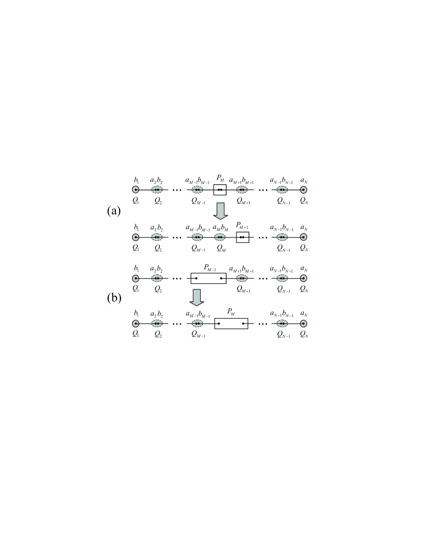
Figure 1: Schematic picture of the DMRG method for the $B\bullet B$ (a) and the $B\bullet\bullet B$ (b) configurations. Horizontal lines represent maximally entangled states $|\phi\rangle$, the ellipses and circles (squares) the operators $Q$ ($P$) which map the auxiliary system into the physical ones.

The more standard scenario ($B\bullet\bullet B$) is represented in Fig. 1(b). The operator $P_{M}$ acts on the auxiliary subsystems $a_{M}$ and $b_{M+1}$ and maps $H_{a}\otimes H_{b}\to H_{M}\otimes H_{M+1}$. In this picture [for both configurations, Figs. 1 (a,b)] it is very clear that the two edge spins are treated on a very different footing since they are represented by a single auxiliary system which is not entangled to any other.

In the case of a problem with PBC a slight modification of the scheme is used WhitePRB . The idea is to still separate the system into two blocks and two spins as before but now with the configuration $B\bullet B\bullet$. This ensures the sparseness of the matrices one has to diagonalize and thus it increases the speed of the algorithm WhitePRB . One can draw the diagram corresponding to this procedure in a similar way as in Fig. 1. The important point is that still there are always two sites (left most and right most of both blocks $B$) which are treated differently since they are represented by a single auxiliary spin which is not entangled to any other. In our opinion, this is the reason of the poor performance of the DMRG method for problems with PBC.

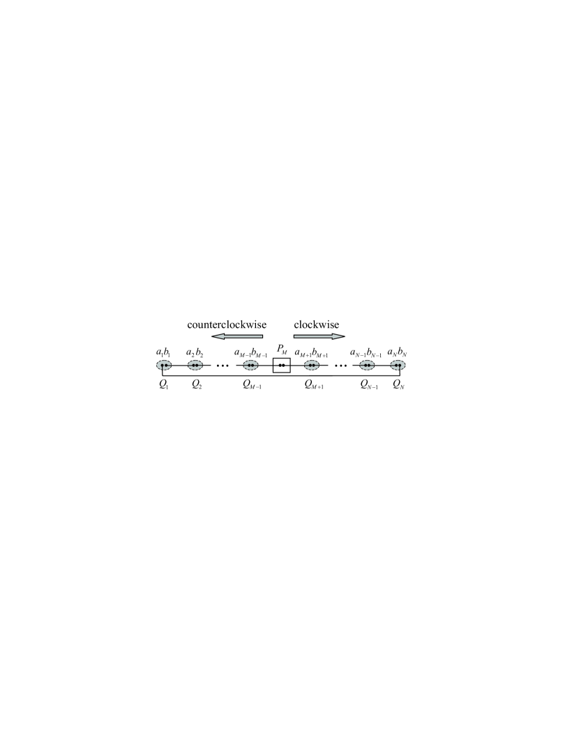
Figure 2: Proposed configurations for the case of PBC. One may also use two spins instead of one

The method we propose is very clear in terms of this picture (Fig. 2). One has to substitute at all sites $k$ the spin by two auxiliary systems $a_{k}$ and $b_{k}$ of dimension $D$, with $b_{k}$ and $a_{k+1}$ (with $a_{N+1}:=a_{1}$) in a maximally entangled states and find the maps $P_{k}:H_{a}\otimes H_{b}\to H_{k}$ which lead to a state

$$|\Psi\rangle=P_{1}\otimes P_{2}\ldots P_{N-1}\otimes P_{N}|\phi\rangle^{\otimes N},$$ (6)

with the minimal energy. This minimization can be performed in a similar way to the one used in the standard DMRG method. Before showing how to do this in practice, we derive some formulas in terms of these operators. We write

$$P_{k}=\sum_{s=1}^{d}|s\rangle\langle\varphi_{s}^{[k]}|,\quad\langle\varphi_{s}^{[k]}|=\sum_{\alpha,\beta}B_{\alpha,\beta}^{[k],s}\langle\alpha,\beta|.$$ (7)

Thus, the problem is solved once the states $\varphi$ (or equivalently, the matrices $B$) are determined. Note that starting from these states, it is possible to calculate expectation values of products of local observables RomerPRL , since

$$\langle\Psi|O_{1}\ldots O_{N}|\Psi\rangle={\rm Tr}\left(E^{[1]}_{O_{1}}\ldots E^{[N]}_{O_{N}}\right),$$ (8)

where

$$E^{[k]}_{O}=\sum_{s,s^{\prime}=1}^{d}\langle s|O|s^{\prime}\rangle B^{[k],s}\otimes\left(B^{[k],s}\right)^{\ast}.$$ (9)

Thus, the main idea to perform the minimization is very simple. Given the Hamiltonian $H$ describing the system, one chooses one site $M$ and writes the energy as

$$E=\frac{\langle\Psi|H|\Psi\rangle}{\langle\Psi|\Psi\rangle}=\frac{\langle\psi^{[M]}|H_{M}|\psi^{[M]}\rangle}{\langle\psi^{[M]}|N_{M}|\psi^{[M]}\rangle},$$ (10)

where $|\psi^{[M]}\rangle=\oplus_{s}|\psi^{[M]}_{s}\rangle$ is a vector built by concatenating the $\psi^{[M]}_{s}$, and $N_{M}$ and $H_{M}$ are $d\times D^{2}$ hermitian square matrices which are built using the vectors $\psi^{[k]}_{s}$ at $k\neq M$. For example, $N_{M}=\oplus_{s}N_{0}$ is a block diagonal matrix with identical blocks $N_{0}$ which has matrix elements $(N_{0})_{(\alpha,\alpha^{\prime}),(\beta,\beta^{\prime})}=(\tilde{N}_{0})_{(\alpha,\beta),(\alpha^{\prime},\beta^{\prime})}$, with

$$\tilde{N}_{0}=E^{[M+1]}_{\bf 1}\ldots E^{[N]}_{\bf 1}E^{[1]}_{\bf 1}\ldots E^{[M-1]}_{\bf 1}.$$ (11)

Thus, at this step the operator $P_{M}$ is found by solving the generalized eigenvalue problem

$$H_{M}|\psi^{[M]}\rangle=\lambda N_{M}|\psi^{[M]}\rangle,$$ (12)

with $\lambda$ minimum, which in turns gives the energy at this step. Then one chooses another site and proceeds in the same way until the energy converges. At the end we have all the $P_{k}$ and can evaluate all expectation values.

The above method is not very efficient numerically. First, the matrix $N_{0}$ may be ill conditioned. Second, one stores many matrices ($\sim N^{2}$) and performs many matrix multiplications ($\sim N^{2}$) at each step. Now we explain how one can make the method much more efficient.

Let assume that we have a set of spins in a ring. The idea is to determine operators $P_{k}$ in a clockwise order (first $P_{1}$, then $P_{2}$, until $P_{N-1}$), then improve them following a counterclockwise ordering (from $P_{N}$ to $P_{2}$), then again clockwise, until the fixed point is reached. At each step, a normalization condition similar to (3) is imposed, depending on whether we are in a clockwise or counterclockwise cycle, which makes the matrix $N_{M}$ well behaved. On the other hand, at each step only the operators which are strictly needed in later steps are calculated in an efficient way and stored.

The normalization condition is based on the following fact. Given the state $\Psi$, characterized by matrices $B$, if we substitute $B^{[M],s}\to B^{[M],s}X:=U^{[M],s}$ and $B^{[M+1],s}\to X^{-1}B^{[M+1],s}$, where $X$ is a nonsingular matrix, we obtain the same state. Analogously, we can substitute $B^{[M],s}\to YB^{[M],s}:=V^{[M]}$ and $B^{[M-1],s}\to B^{[M-1],s}Y^{-1}$. We choose $X$ in the clockwise cycles to impose (3) and $Y$ in the counterclockwise ones to impose

$$\sum_{s=1}^{d}\left(V^{[M],s}\right)^{\dagger}\left(V^{[M],s}\right)={\bf 1}.$$ (13)

Thus, at the point of determining the operator $P_{M}$,

$$|\Psi\rangle=Q_{1}\otimes\ldots Q_{M-1}\otimes P_{M}\otimes\tilde{Q}_{M+1}\ldots\otimes\tilde{Q}_{N}|\phi\rangle^{\otimes N},$$ (14)

where $Q_{k}$ and $\tilde{Q}_{k}$ are defined as in (7) but with $U$ and $V$ instead of $B$, respectively. Thus, the operators $X$ and $Y$ are all of them moved over, such that they are now included in those corresponding to $P_{M}$. It can be easily shown that these conditions on the operator $U$ ($V$) are equivalent to imposing that $E_{\bf 1}$ has the maximally entangled state $|\phi\rangle$ as right (left) eigenvector with eigenvalue 1. This is immediately reflected in the fact that the matrix $N_{M}$ is better behaved, which makes the problem numerically stable.

Let us now illustrate how the procedure works with simplest nearest neighbor Hamiltonian $\sigma_{z}^{[k]}\sigma_{z}^{[k+1]}$, namely the Ising Model. Let us assume that we are running the optimization of the operators clockwise and that we want to determine $P_{M}$. So far, in previous steps, apart from the matrices $U$ and $V$, we have stored: (a) For each $k<M$, the following four operators:

$$r_{k} := E_{\bf 1}^{[1]}E_{\bf 1}^{[2]}\ldots E_{\bf 1}^{[k-2]}E_{\bf 1}^{[k-1]},$$ (15a)

$$s_{k} := E_{\sigma_{z}}^{[1]}E_{\bf 1}^{[2]}\ldots E_{\bf 1}^{[k-2]}E_{\bf 1}^{[k-1]},$$ (15b)

$$t_{k} := E_{\bf 1}^{[1]}E_{\bf 1}^{[2]}\ldots E_{\bf 1}^{[k-2]}E_{\sigma_{z}}^{[k-1]},$$ (15c)

$$h_{k} := \sum_{n=1}^{k-2}E_{\bf 1}^{[1]}E_{\bf 1}^{[2]}\ldots E_{\sigma_{z}}^{[n]}E_{\sigma_{z}}^{[n+1]}\ldots E_{\bf 1}^{[k-2]}E_{\bf 1}^{[k-1]},$$ (15d)

(b) For each $k>M$ other four similar operators which contain products from $E^{[k]}$ to $E^{[N]}$. With them, one can build $H_{M}$ and $N_{0}$ by few matrix multiplications and thus determine $P_{M}$ by solving (12). From it, $Q_{M}$ is determined. Then, we construct $r_{M+1},s_{M+1},t_{M+1}$ and $h_{M+1}$ starting from $r_{M},s_{M},t_{M}$ and $h_{M}$ note2 . We continue in the same vein, finding four matrices at each step, and storing them, until we reach $N$. Then we start moving counterclockwise and start constructing the corresponding four matrices at each step. Notice that in order to construct the matrices $H_{M}$ and $N_{0}$ we will have to use the stored matrices (15) which were determined when we were moving clockwise. Thus, with this procedure we have to store of the order of $4N$ matrices of dimension $D^{2}$ (apart from the matrices $U$, $V$ and the last $B$’s) but the number of operations per step is independent of $N$. At the end, when we have reached the fixed point, we can determine the expectation value of any operator by using (8) and determining the required matrices using (9). Note that if the problem has translational symmetry, then all these evaluations are even simpler.

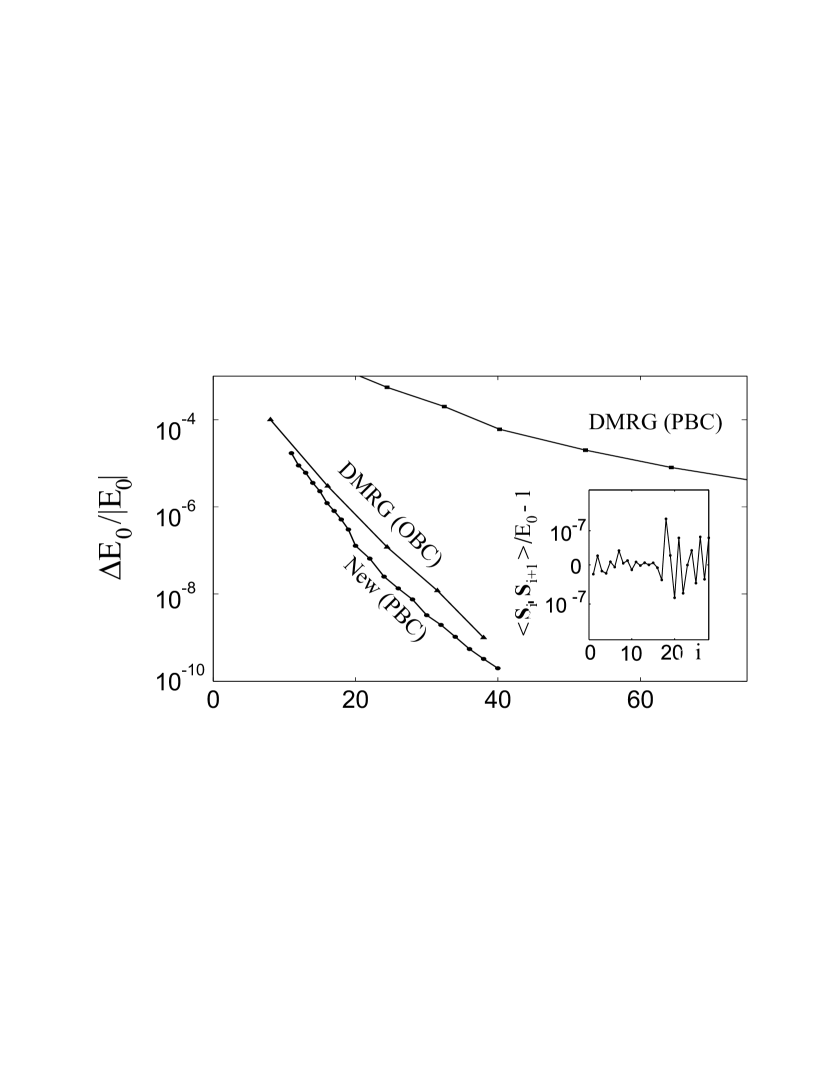
Figure 3: (Left) Comparison between DMRG (squares) WhitePRB and the new method (circles) for PBC, and $N=28$. For reference the DMRG results WhitePRB for the Heisenberg chain with OBC (triangles) are also shown. (Insert) Variation of the local bond strength from the average along the chain, calculated with the new method and $D=40$.

We have applied the above method to the spin $1/2$ Heisenberg chain. We have plotted in Fig. 3 the energies obtained as a function of $D$ and compared them with those obtained by the standard DMRG method with OBC and PBC. From the figure it is clear that the accuracies we obtain are comparable with those obtained with DMRG for problems with OBC but much better than for PBC. We have determined the errors by comparing with the exact results Exact . In the insert of Fig. 3 we have plotted the local bond strength $\langle{\mathbf{S}}^{[k]}{\mathbf{S}}^{[k+1]}\rangle$ as a function of $k$. As expected, the result is independent of the position $k$, as opposed to what occurs with OBC.

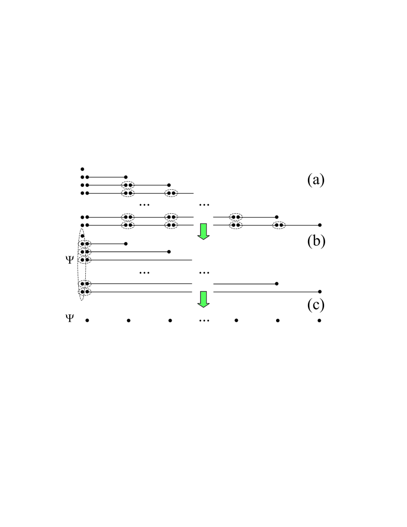
Figure 4: General states can be expressed in the form (6).

Finally we show that the picture introduced here may be valuable to understand the properties of states $\Psi$ in terms of the language and tools developed in the field of QIT. First, one can easily see that the entropy of the block formed by systems $(k_{0},k_{0}+1,\ldots,k_{1})$ is bounded by $2\log_{2}(D)$, as this block is connected to the rest only via $a_{k_{0}}$ and $b_{k_{1}+1}$, and thus the rank of the reduced density operator for the block is bounded by the product of the dimensions of the corresponding Hilbert spaces. Secondly, it allows us to show that any state can be written in the form (6) (MPS Fannes ; RomerPRL ) if we choose $D=d^{N}$ (actually, $D=d^{\lfloor\frac{N}{2}\rfloor}$ is sufficient). We consider $a_{k}$ and $b_{k}$ as composed of $d$–level subsystems, $a_{k}^{1},\ldots,a_{k}^{N}$ and $b_{k}^{1},\ldots,b_{k}^{N}$, respectively, and write $|\phi\rangle$ as a tensor product of maximally entangled states $\phi_{d}$ between $b_{k}^{l}$ and $a_{k+1}^{l}$. For $k=2,\ldots,N$, we choose the operators $P_{k}={\bf 1}_{a_{k}^{k}}\otimes\langle\eta_{k}|$ where $|\eta_{k}\rangle$ is a state for all particles but $a_{k}^{k}$, and contains $|\phi_{d}\rangle$ for each pair $a_{k}^{l}$-$b_{k}^{l}$ ($l>k$) and $|0\rangle$ for the rest. The action of $P_{k}$ is to teleport the entangled pairs such that at the end one has one entangled pairs between the first system and all the rest (Fig. 4), while leaving all the other auxiliary particles in $|0\rangle$. Finally, the operator $P_{1}$ is the product of two operators. The first acts on particles $a_{1}$ and transforms $|0\rangle^{N}\to|\Psi\rangle$. The second is ${\bf 1}_{a_{1}^{1}}\otimes\langle\eta_{1}|$, where $|\eta_{1}\rangle=|0\rangle_{b_{1}}\otimes|\phi_{d}\rangle^{\otimes N-1}$. This operator first prepares the desired state $\Psi$ in particles $a_{1}$ and then uses the available entangled pairs to teleport it to the the rest of the particles.

In summary, we have given a pictorial view of the DMRG method and have identified the reason of its poor performance for problems with PBC. Our picture immediately leads to a modified version of the DMRG method which dramatically improves the results. This is done at the expenses of no longer using sparse matrices, something which limits its applications. Nevertheless, we believe that the method may allow us to treat problems in condensed matter systems which so far have been difficult to tackle with the standard DMRG method. In any case, the present work illustrates how the developments made in QIT during the last years may prove useful in other branches of Physics.

We thank M.A. Martin-Delgado for enlightening discussions about DMRG and G. Cabrera for sending the extended data of Exact . Work supported by the DFG (SFB 631), the european project and network Quprodis and Conquest, and the Kompetenznetzwerk der Bayerischen Staatsregierung Quanteninformation.

References

- (1) S.R.White, Phys. Rev. Lett. 69, 2863 (1992).
- (2) S.R.White, Phys. Rev. B 48, 10345 (1992).
- (3) See, for example, Density–Matrix Renormalization, Eds. I. Peschel, et al., (Springer Verlag, Berlin, 1999).
- (4) S. Ostlund and S. Rommer, Phys. Rev. Lett. 75, 3537 (1995); S. Rommer and S. Ostlund, Phys. Rev. B 55, 2164 (1997).
- (5) J. Dukelsky et al., Europhys. Lett. 43, 457 (1997).
- (6) M. Fannes, B. Nachtergaele and R.F. Werner, Comm. Math. Phys. 144, 443 (1992).
- (7) C. H. Bennett et al., Phys. Rev. Lett. 70, 1895 (1993).
- (8) M. Nielsen and I. Chuang, Quantum Computation and Quantum Information, Cambridge University Press (2000).
- (9) G. Vidal et al., Phys. Rev. Lett. 90, 227902 (2003).
- (10) F. Verstraete, M. Popp, and J. I. Cirac, Phys. Rev. Lett. 92, 027901 (2004); F. Verstraete, M. A. Martin-Delgado, and J. I. Cirac, Phys. Rev. Lett. 92, 087201 (2004),
- (11) T. J. Osborne and M. A. Nielsen, Phys. Rev. A 66, 032110 (2002).
- (12) G. Vidal, Phys. Rev. Lett. 91, 147902 (2003).
- (13) I. Affleck et al., Commun. Math. Phys. 115, 477 (1988).
- (14) Note that this it is always possible to consider the first and last spins as two larger spins. Here is the minimum integer such that .
- (15) H. Takasaki, T. Hikihara, and T. Nishino, J. Phys. Soc. Jpn. 68, 1537 (1999).
- (16) Note that this can be done more efficiently by using the fact that the matrices have at most rank 2.
- (17) D. Medeiros and G.G. Cabrera, Phys. Rev. B 43, 3703 (1991).