Phase diagram of a frustrated mixed-spin ladder with diagonal exchange bonds

Abstract

Using exact numerical diagonalization and the conformal field theory approach,, we study the effect of magnetic frustrations due to diagonal exchange bonds in a system of two coupled mixed-spin $(1,\frac{1}{2})$ Heisenberg chains. It is established that relatively moderate frustrations are able to destroy the ferrimagnetic state and to stabilize the critical spin-liquid phase typical for half-integer-spin antiferromagnetic Heisenberg chains. Both phases are separated by a narrow but finite region occupied by a critical partially-polarized ferromagnetic phase.

I Introduction

Many experiments on bimetallic quasi-one-dimensional (1D) molecular magnets imply that the magnetic properties of these compounds are basically described by the Heisenberg spin model with antiferromagnetic exchange couplings. kahn ; hagiwara In the last decade, there has been an increasing experimental and theoretical interest in these mixed-spin systems exhibiting intriguing quantum spin phases and thermodynamic properties. In particular, a number of recent studies has been focused on ground-state properties of mixed-spin ladders. senechal

In this paper we study the ground-state phase diagram of a ferrimagnetic two-leg ladder containing frustrating antiferromagnetic diagonal exchange bonds (see Fig. 1). The model is defined by the Hamiltonian

$${\cal H}=\sum_{n=1}^{L}\left[J_{1}\left({{\bf s}_{1}}_{n}\cdot{{\bf s}_{2}}_{n+1}+{{\bf s}_{2}}_{n}\cdot{{\bf s}_{1}}_{n+1}\right)+J_{\perp}{{\bf s}_{1}}_{n}\cdot{{\bf s}_{2}}_{n}\right]\\ +J_{2}\sum_{n=1}^{L}\left({{\bf s}_{1}}_{n}\cdot{{\bf s}_{1}}_{n+1}+{{\bf s}_{2}}_{n}\cdot{{\bf s}_{2}}_{n+1}\right)\,,$$ (1)

where $L$ is the number of rungs and the spin operators ${{\bf s}_{1}}_{n}$ and ${{\bf s}_{2}}_{n}$ are defined on the rung with index $n$: $\left({{\bf s}_{1}}_{n}\right)^{2}=s_{1}(s_{1}+1)$, $\left({{\bf s}_{2}}_{n}\right)^{2}=s_{2}(s_{2}+1)$, $s_{1}>s_{2}$, and $J_{1},J_{2},J_{\perp}>0$. We introduce the frustration parameter $\alpha=J_{2}/J_{1}$, the spin ratio $\sigma=s_{1}/s_{2}$, and set the energy and length scales by $J_{1}\equiv 1$ and $a_{0}=1$, where $a_{0}$ is the spacing between neighboring rungs. In the remainder of this paper, if not especially noted, we will consider the case $J_{\perp}=J_{1}$.

As a function of the frustration parameter $\alpha$, the classical phase diagram of (1) exhibits three phases described by the angles $(\theta,\phi)$ fixing the directions of the classical spins ${{\bf s}_{1}}_{n}$ and ${{\bf s}_{2}}_{n}$ in respect to the classical ferrimagnetic configuration with spins ${{\bf s}_{1}}_{n}$ and ${{\bf s}_{2}}_{n}$ oriented along the axes ${\bf z}_{1}$ and ${\bf z}_{2}$, respectively (Fig. 1). The classical canted state (C) shown in Fig. 1 is stable in the interval $\alpha_{c1}<\alpha<\alpha_{c2}$ where $\alpha_{c1}=3[(\sigma^{2}+1)-\sqrt{(\sigma^{2}+1)^{2}-32\sigma^{2}/9}]/8\sigma$ and $\alpha_{c2}=[-(\sigma^{2}+1)+\sqrt{(\sigma^{2}+1)^{2}+32\sigma^{2}}]/8\sigma$ are second-order phase transition points separating the C phase from the ferrimagnetic (F) $(\theta,\phi)=(0,0)$ and the mixed-spin collinear $(\theta,\phi)=(\pi/2,\pi/2)$ phases, respectively. In the case of special interest $(s_{1},s_{2})=(1,\frac{1}{2})$, the classical transition points are $\alpha_{c1}=0.3219$ and $\alpha_{c2}=0.4606$. Notice that the square-lattice $J_{1}-J_{2}$ mixed-spin Heisenberg modelivanov1 exhibits similar classical magnetic phases which persist in the quantum phase diagram. On the other hand, the following analysis of (1) implies that in one space dimension the ferrimagnetic phase continues to exist in the quantum phase diagram, whereas the classical collinear magnetic state is completely destroyed by quantum fluctuations. Instead, for $\alpha>\alpha_{2c}$ there appears a singlet quantum paramagnetic phase which is critical (gapped) for half-integer (integer) rung spins ${\bf S}_{n}={{\bf s}_{1}}_{n}+{{\bf s}_{2}}_{n}$. As to the classical canted phase, it is argued that the longitudinal ferromagnetic order survives quantum fluctuations. On the other hand, on general grounds we may expect that the transverse magnetic ordering does not survive quantum fluctuations. A closely related phase diagram appears in a special class of lattice models with quantum-rotor degrees of freedom.sachdev

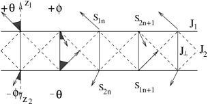
Figure 1: Sketch of the classical canted state for $J_{\perp}=J_{1}$ described by the angles $(\pm\theta,\pm\phi)$ for every magnetic cell composed of two neighboring rungs. $\theta$ and $\phi$ measure the deviations of the classical spins from the ferrimagnetic configuration: ${{\bf s}_{1}}_{n}\|{\bf z}_{1}$ and ${{\bf s}_{2}}_{n}\|{\bf z}_{2}$.

The following analysis of the quantum phase diagram is performed by using exact numerical diagonalization (ED) of small periodic systems, finite-size analysis of the ED data, and analytical spin-wave calculations. The emphasis is on the properties of the quantum paramagnetic phase.

II Magnetic phases

As may be expected, the positions of the classical phase transition points $\alpha_{c1}$ and $\alpha_{c2}$ are changed by quantum spin fluctuations. Using ED and a simple finite-size scaling, it is possible to find precise estimates for the quantum transition points. The latter are connected with the following changes in the total spin of the ground state $S_{T}$: $S_{T}=(s_{1}-s_{2})L$ for $0\leq\alpha<\alpha_{c1}$ (F phase), $0<S_{T}<(s_{1}-s_{2})L$ for $\alpha_{c1}<\alpha<\alpha_{c2}$ (C phase), and $S_{T}=0$ for $\alpha>\alpha_{c2}$ (quantum paramagnetic phase). The extrapolated data for $L=8,10,12$, and $14$ give the results $\alpha_{c1}=0.341$ and $\alpha_{c2}=0.399$ showing that the region occupied by the quantum C phase is narrowed but definitely finite. Figure 2 provides a summary of the reported results in terms of the net ferromagnetic moment per rung $M_{0}$ for $L=12$.

Figure 2: ED results for the ferromagnetic moment per rung $M_{0}$ $vs$ $J_{2}/J_{1}$ (dashed line). The step-like form of $M_{0}(J_{2}/J_{1})$ is connected to finite-size effects. The midpoints of the steps close to $\alpha_{c2}$ are well approximated by the ansatz $M_{0}=m_{1}(\alpha_{c2}-\alpha)^{\beta}+m_{2}(\alpha_{c2}-\alpha)$, where $m_{1}=1.65,m_{2}=0.56$, and $\beta=\frac{1}{2}$ (solid line).

The ferrimagnetic phase has already been studied for the model (1) without frustration.ivanov2 As $M_{0}>0$, both magnetic phases (F and C) are characterized by quadratic spin-wave excitations

$$E(k)=\frac{\rho_{s}}{M_{0}}k^{2}+{\cal O}(k^{4})\,,$$ (2)

where $\rho_{s}$ is the ferromagnetic spin-stiffness constant.halperin In approaching $\alpha_{c1}$ from the ferrimagnetic phase, the linear spin-wave theory predicts that the lower spin wave branch softens in the vicinity of $k=\pi$ and the gap at this point vanishes for $\alpha>\alpha_{c1}$. Thus the linear Goldstone mode, characteristic of the classical C phase, seems to survive quantum fluctuations although on general grounds it may be expected that the spin rotation symmetry $U(1)$ in the $xy$ plane is restored in one space dimension, i.e., $\langle{s_{1}}_{n}^{x}\rangle=\langle{s_{2}}_{n}^{x}\rangle=0$. note1 This scenario is supported by the renormalization-group analysis of similar phases in quantum rotor models,sachdev implying that the true tranverse long-range magnetic order in the classical C phase is transformed to a quasi-long-range $xy$ order in the quantum system. On the other hand, the spin-stiffness constant $\rho_{s}$ remains finite in both magnetic phases as well as at the transition point $\alpha_{c1}$. Following the terminology of Ref. sachdev, , the quantum C phase may be called partially polarized ferromagnetic phase, as the ferromagnetic moment $M_{0}$ is less than the maximal value $s_{1}-s_{2}$ in the ferrimagnetic phase (see Fig. 2). This quantum state may also be classified as a kind of ferromagnetic Luttinger liquid.bartosch We postpone the detail analysis of this quantum phase for future studies.

III Quantum paramagnetic phase

Now, let us turn to the region $\alpha>\alpha_{c2}$ of the phase diagram characterized by $S_{T}=0$. It is instructive to rewrite (1) in the following form

$${\cal H}=\sum_{n=1}^{L}\left(J_{1}{\bf S}_{n}\cdot{\bf S}_{n+1}+J_{\perp}{{\bf s}_{1}}_{n}\cdot{{\bf s}_{2}}_{n}\right)\\ +(J_{2}-J_{1})\sum_{n=1}^{L}\left({{\bf s}_{1}}_{n}\cdot{{\bf s}_{1}}_{n+1}+{{\bf s}_{2}}_{n}\cdot{{\bf s}_{2}}_{n+1}\right)\,.$$ (3)

The operator $2{{\bf s}_{1}}_{n}\cdot{{\bf s}_{2}}_{n}=\left({\bf S}_{n}\right)^{2}-s_{1}(s_{1}+1)-s_{2}(s_{2}+1)$ is a conserved quantity for $J_{2}=J_{1}$ and at this special point the low-energy physics of (1) is described by the antiferromagnetic spin-$S$ Heisenberg chain: $\left({\bf S}_{n}\right)^{2}=S(S+1),S=s_{1}-s_{2},s_{1}-s_{2}+1,\ldots,s_{1}+s_{2}$. In the case of special interest $(s_{1},s_{2})=(1,\frac{1}{2})$, and for relatively small interchain couplings $J_{\perp}\lessapprox 1.59J_{1}$, we have numerically found that all the rung spins are characterized by $S=\frac{3}{2}$, so that in the low-energy sector the ladder model (1) is equivalent to the $S=\frac{3}{2}$ antiferromagnetic Heisenberg chain.

Figure 3: ED results for the lowest excited states of the system $(s_{1},s_{2})=(1,\frac{1}{2})$ for two different frustration parameters ($\alpha=1$ and $0.4$): $L=12$ (open circles), $L=14$ (filled circles). Curves represent the two branches of spin-wave modes in the paramagnetic Brillouin zone, as obtained from the linear spin-wave theory. The spin-wave energies are multiplied by the normalization factor $v_{s}/v_{sw}=1.29$ where $v_{s}=3.87$ and $v_{sw}=2S=3$ are the spin-wave velocities, as obtained by the density matrix renormalization group methodhallberg and the linear spin-wave theory. Note that the classical transition point at $\alpha=0.4606$ appears as an instability point for the lower spin-wave branch.

The above statements concern the special point $J_{2}=J_{1}$ where $S$ is a good quantum number. As an example, in Fig. 3 we show the energies of the lowest excited states ($L=12$ and $14$) for $\alpha=0.4$ and $1$. Apart from the $k=0$ state, which is characterized by the total spin $2$, the lowest excited states are triplets above the singlet ground state. This structure of the low-energy spectrum is valid in the whole region $\alpha>\alpha_{c2}$ up to the limit $\alpha=\infty$ where the system is composed of two independent $s_{1}=1$ and $s_{2}=\frac{1}{2}$ antiferromagnetic Heisenberg chains. In accord to the generalized Lieb-Schultz-Mattis (LSM) theorem, affleck2 it is natural to suppose that the gapless linear structure of the spectrum around $k=\pi$ survives away from the point $J_{2}=J_{1}$.

To study the properties of the quantum paramagnetic phase in the whole region $\alpha>\alpha_{c2}$, we may compare the finite-size scaling properties of the ground state and the lowest excited states with those based on the $SU(2)$ Wess-Zumino-Witten (WZW) nonlinear $\sigma$ model. This model with the topological coupling $k_{0}=1$ is believed to describe the antiferromagnetic Heisenberg chains with half-integer site spins. affleck1 . In the following we restrict our analysis to the $(s_{1},s_{2})=(1,\frac{1}{2})$ system. According to the conformal field theory, the ground state energy $E_{0}(L)$ of a periodic system with length $L$ is given by the following expressionaffleck1

$$\frac{E_{0}}{L}=\varepsilon_{0}-\frac{\pi v_{s}}{6L^{2}}\left[1+\frac{3}{8}g^{3}+{\cal O}(g^{4})\right]+\frac{a_{1}}{L^{4}}\,.$$ (4)

Here $\varepsilon_{0}$ is the ground state energy per rung in the thermodynamic limit, $v_{s}$ is the spin-wave velocity, and $g=g(L)$ is the effective coupling constant of the marginally irrelevant operator $-2\pi g{\bf J}_{L}\cdot{\bf J}_{R}$ at the length scale $L$. ${\bf J}_{L}$ and ${\bf J}_{R}$ are the conserved current operators for the left and right movers in the WZW theory. The $L^{-4}$ contribution comes from irrelevant operators. The coupling $g$ is defined by the renormalization-group (RG) equationsolyom ; lukyanov

$$\frac{1}{g}+\frac{1}{2}\ln g=\ln\frac{L}{L_{c}}\,,$$ (5)

where $L_{c}$ is a non-universal effective length scale depending on the microscopic model. An iterative solution of (5) yields the following expansion for $g$

$$g=\frac{1}{\ln(L/L_{c})}-\frac{\ln\ln(L/L_{c})}{2\ln^{2}(L/L_{c})}+{\cal O}\left(\frac{1}{\ln^{3}(L/L_{c})}\right)$$ (6)

so that the marginally irrelevant operator introduces logarithmic corrections in Eq. (4).

The energy of the lowest triplet excitation $E_{t}(L)$ with momentum $k=\pi$ can be expressed in the form

$$\frac{E_{t}-E_{0}}{L}=\frac{2\pi v_{s}}{L^{2}}\left[\frac{1}{2}-\frac{g}{4}+b_{1}g^{2}+{\cal O}(g^{3})\right]+\frac{b_{2}}{L^{4}}\,.$$ (7)

At moderate length scales ($L$=8,10,12, and 14), the coupling constants $g(L)$ in (4) and (7) may have different values, so that instead of $L_{c}$ we introduce the effective length scales $L_{0}$ and $L_{t}$ for the ground state energy and the energy of triplet excitations.

Figure 4: Reduced energy gap between the lowest excited state at $\pi-2\pi/L$ and the ground state. The interpolation of ED data is performed by the ansatz $E(2\pi/L)/2\pi L=\sum_{n=1}^{3}c_{n}L^{-2n}$. For $\alpha=0.45,0.5$, and $1$ this yields, respectively, the spin-wave velocities $v_{s}=1.19,1,78$, and $3.81$. Note that the interpolation function for $\alpha=0.4$ has a positive curvarute.

The parameter $v_{s}$ in Eqs. (4) and (7) can be independently determined from the scaling of the reduced gap $E(2\pi/L)/2\pi L$, where $E(2\pi/L)$ is the energy gap between the lowest excited state with momentum $\pi-2\pi/L$ and the ground state. Using the interpolation ansatz $E(2\pi/L)/2\pi L=\sum_{n=1}^{3}c_{n}L^{-2n}$, we find, in particular, the estimate $v_{s}\equiv c_{1}=3.81$ at $\alpha=1$. This is close to the density matrix RG result $3.87\pm 0.02$ for the antiferromagnetic $S=\frac{3}{2}$ Heisenberg chain. hallberg In Fig. 4 we present the interpolation curves for different values of the frustration parameter $\alpha$. Excluding the point $\alpha=0.4$, our estimates for $v_{s}$ can be well interpolated by the ansatz

$$v_{s}=v_{1}(\alpha-\alpha_{2c})^{\gamma}+v_{2}(\alpha-\alpha_{2c})+{\cal O}\left[(\alpha-\alpha_{2c})^{2}\right]$$ (8)

up to $\alpha=1$, provided that $\gamma\approx\frac{2}{3}$. The linear spin-wave theory gives the exponent $\gamma=\frac{1}{2}$. Note that the spin-wave ansatz (8) assumes that the velocity $v_{s}$ vanishes at the critical point $\alpha_{c2}$. Of course, the above interpolation of ED data can not definitely confirm such an assumption, although the apparent change in the curvature of $E(2\pi/L)/2\pi L$ $vs$ $1/L^{2}$ close to $\alpha=0.4$ gives some indication in favor of $v_{s}(\alpha_{c2})=0$.cabra

Figure 5: Scaling of the ground state energy $E_{0}(L)/L$ at $\alpha=0.45$ and $0.5$. The interpolation of ED data is performed by Eqs. (4) and (5).

Having the parameter $v_{s}$ for different $\alpha$, now we can interpolate the ED data for $E_{0}(L)$ and $E_{t}(L)$ by using the scaling expressions (4) and (7). The fitting parameters in (4) are $\varepsilon_{0}$, $a_{1}$ and $L_{0}$. Alternatively, in Eq. (7) the fitting parameters are $b_{1}$, $b_{2}$, and $L_{t}$. As an example, in Fig. 5 we present the interpolation curves $E_{0}(L)/L$ $vs$ $1/L^{2}$ for frustration parameters $\alpha=0.45$ and $0.5$. Using the RG equation (5) for $g(L)$, the best fit at $\alpha=1$ is obtained for $\varepsilon_{0}=-2.3290$, $L_{0}=0.94$ and $a_{1}=-20.5$. This is in accord with the density matrix RG result $\varepsilon_{0}=-2.32833$. hallberg The parameter $L_{0}=0.94$ corresponds to an effective coupling constant $g(10)=0.35$. Performing the fits down to $\alpha=0.4$, we observe that the characteristic length $L_{0}$ remains almost unchanged (excluding the point $\alpha=0.4$ where formally $L_{0}\rightarrow\infty$). An interpolation procedure using only the leading term in the logarithmic expansion (6) produces similar results, although with a slightly larger effective length $L_{0}$ ($=1.08$).

Figure 6: Scaling of the triplet gap $\Delta_{t}/L=[E_{t}(L)-E_{0}(L)]/L$ for the frustration parameters $\alpha=0.42,0.45,0.5$, and $1$. The fit of ED data is performed with the scaling formula (7) and by using the logarithmic expansion (6) up to second order in $1/\ln(L/L_{t})$.

Table 1: Values of the coefficients in (4) and (7) giving the best fit to the ED data. The values of $v_{s}$ correspond to the ansatz (8) with $\gamma=\frac{2}{3}$ giving the best fit to the estimates from Fig. 4. $L_{0}=0.94$ for all values of $\alpha$ presented in the Table.

$\alpha$	$v_{s}$	$\varepsilon_{0}$	$a_{1}$	$L_{t}$	$b_{1}$	$b_{2}$
0.42	0.71	-1.5608	-26.8	2.20	-2.2	318
0.45	1.21	-1.5873	-26.0	2.20	-1.8	449
0.50	1.77	-1.6373	-25.5	2.12	-1.5	495
1.00	3.87	-2.3290	-20.5	2.06	-1.4	942

The ${\cal O}(g)$ correction to the scaling dimension in (7) makes the fit of our ED data more intricate. Moreover, we have found that for $L\leq 14$ the lowest singlet excited states $E_{s}(L)$ may belong to different conformal towers. That is why, instead of utilizing the combination of $E_{t}(L)$ and $E_{s}(L)$ which eliminates the ${\cal O}(g)$ correction, ziman we have performed the interpolation directly with Eq. (7) by using the logarithmic expansion (6) up to second order in $1/\ln(L/L_{t})$. The results presented in Fig. 6 and Table 1 imply that the effective coupling at a given length scale $g(L)$ exhibits only a small increasenote2 when approaching the critical point $\alpha_{c2}$, in agreement with the interpolation result for $E_{0}(L)$. On the other hand, as $\alpha\rightarrow\alpha_{c2}$ one indicates a monotonous growth of the ${\cal O}(g^{2})$ contribution to the scaling dimension. The scaling behavior of $E_{0}(L)$ and $E_{t}(L)$ for $\alpha>1$ qualitatively reveals the same properties.

IV Conclusions

In conclusion, we have examined the impact of magnetic frustration on the ground-state phase diagram of two coupled mixed-spin $(s_{1},s_{2})=(1,\frac{1}{2})$ ferrimagnetic Heisenberg chains. The analysis of ED data implies an interesting phase diagram containing the ferrimagnetic phase and a singlet paramagnetic phase exhibiting the characteristics of the critical spin-liquid phase in half-integer-spin antiferromagnetic Heisenberg chains. Both phases are separated by a tiny but finite region occupied by a critical partially-polarized ferromagnetic phase. It is natural to expect similar phase diagrams for the whole class of frustrated $(s_{1},s_{2})$ two-leg ladders with half-integer rung spins.

- (1) O. Kahn, Y. Pei and Y. Journaux: Molecular Inorganic Magnetic Materials. In: Inorganic Materials, ed by D.W. Bruce, D. O’Hare ( John Wiley Sons, New York 1992).
- (2) M. Hagiwara, K. Minami, Y. Narumi, K. Tatani, and K. Kindo, J. Phys. Soc. Jpn. 67, 2209 (1998); ibid. 68, 2214 (1999); N. Fujiwara and M. Hagiwara, Sol. State Commun. 113, 443 (2000).
- (3) D. Sénéchal, Phys. Rev. B 52, 15319 (1995); A.K. Kolezhuk and H.-J. Mikeska, Eur. Phys. J. B 5, 543 (1998); A. Koga, S. Kumada, N. Kawakami, and T. Fukui, J. Phys. Soc. Jpn. 67, 622 (1998); A. Satou and Y. Nakamura, ibid. 68, 4014 (1999); A. Langari and M.A. Martin-Delgado, Phys. Rev. B 63, 054432 (2001); A.E. Trumper and C. Gazza, ibid. 64, 134408 (2001); J. Lou, Ch. Chen, and Sh. Qin, ibid. 64, 144403 (2001); ibid. 67, 064419 (2003); O. Rojas and F.C. Alcaraz, ibid. 67, 174401 (2003).
- (4) N.B. Ivanov, J. Richter, and D.J.J. Farnell, Phys. Rev. B 66, 014421 (2002).
- (5) S. Sachdev and T. Senthil, Ann. Phys. (N.Y.) 251, 76 (1996).
- (6) N.B. Ivanov and J. Richter, Phys. Rev. B 63, 1444296 (2001).
- (7) B.I. Halperin and P.C. Hohenberg, Phys. Rev. 188, 898 (1969).
- (8) For brevity, we do not present the ED data revealing the anisotropy in the spin-spin correlations in both magnetic phases.
- (9) See, e.g., L. Bartosch, M. Kollar, and P. Kopietz, Phys. Rev. B 67, 092403 (2003), and references therein.
- (10) I. Affleck, D. Gepner, H.J. Schultz, and T. Ziman, J. Phys. A: Math. Gen, 22, 511 (1989).
- (11) Note that the -th unit cell of the model (1) contains only the rung spins and so that for we can apply the generalized LSM theorem: see, Affleck and E. Lieb, Lett. Math. Phys. 12, 57 (1986).
- (12) K. Hallberg, X.Q.G. Wang, P. Horsch, and A. Moreo, Phys. Rev. Lett. 76, 4955 (1996).
- (13) S. Lukyanov, Nucl. Phys. B 522, 533 (1998).
- (14) J. Solyom, Adv. Phys. 28, 201 (1979).
- (15) The assumption has also been considered as a general criterion for ferromagnetic instabilities in the critical paramagnetic phase: see, D.C. Cabra and J.E. Drut, J. Phys.: Condens. Matter 15, 1445 (2003), and references therein.
- (16) T. Ziman and H.J. Schulz, Phys. Rev. Lett. 59, 140 (1987).
- (17) Respectively, the effective coupling constant increases from at up to at .