On the origin of temperature dependence of interlayer exchange coupling in metallic trilayers

Abstract

We study the influence of collective magnetic excitations on the interlayer exchange coupling (IEC) in metallic multilayers. The results are compared to other models that explain the temperature dependence of the IEC by mechanisms within the spacer or at the interfaces of the multilayers. As a main result we find that the reduction of the IEC with temperature shows practically the same functional dependence in all models. On the other hand the influence of the spacer thickness, the magnetic material, and an external field are quite different. Based on these considerations we propose experiments, that are able to determine the dominating mechanism that reduces the IEC at finite temperatures.

I introduction

A lot of aspects of the coupling of two magnetic layers separated by a paramagnetic, metallic spacer are well understood todayBru95 . The coupling is caused by spin dependent reflections of spacer electrons at the interfaces. It oscillates with the spacer thickness $D$. The periods are determined by the spacer, namely by stationary Fermi surface spanning vectors in growth direction. This are vectors parallel to the film normal that connect two points on the Fermi surface and have a vanishing first derivative with respect to the planar components of the Fermi vectors.
However, the origin of the temperature dependence is still under discussion. Up to now it is not clear if the temperature dependence is governed by effects within the spacer, at the interface or within the magnetic layers. There are several proposals for mechanisms reducing the coupling at finite temperatures.

• spacer contribution
  One reason of the reduced IEC is the softening of the Fermi edge at higher temperatures, which makes the coupling mechanism less effective. This was proposed by Bruno and Chappert BrC91 and Edwards et.al. EMM91 It leads to a certain temperature dependent factor for each oscillation period.

• interface contribution
  The argument $\phi_{\sigma}$ of the complex reflection coefficients $r_{\sigma}=|r_{\sigma}|e^{i\phi_{\sigma}}$ at the spacer/magnet interface may be highly energy dependent. This gives rise to an additional temperature dependence of the IEC since the energy interval of interest around the Fermi energy increases with temperatureAMV96 ; CAF99 . The same may in principle apply to the norm of $r_{\sigma}$Bru99 . A rather obvious effect is the reduction of the spin asymmetry of the reflection coefficient $\Delta r=r_{\uparrow}-r_{\downarrow}$ with temperature.

• magnetic layers
  Collective excitations within the magnetic layers reduce their free energy. Since the layers are coupled the excitations depend on the angle between the magnetization vectors of both layers. Thus the reduction of the free energy will be different for parallel and antiparallel alignment of the magnetic layers. This difference

  $$\Delta F_{\rm mag}(T)=F_{\rm mag}^{\uparrow\uparrow}(T)-F_{\rm mag}^{\uparrow\downarrow}(T)$$

  contributes to the temperature dependence of the IEC.
  

The first two contributions are closely associated with the coupling mechanism. The third effect works rather parallel to the coupling mechanism itself, but nevertheless has consequences for the amount of energy achieved by the coupling.
It is the aim of this paper to study the role of the different contributions to the temperature dependence of the IEC. Thereto we have to gain explicit expressions for case (iii). The first two contributions can be described in the frame of ab initio theory combined with Fermi liquid theoryKDT00 ; DKB99 as well as in an quantum well pictureBru95 . They are thoroughly discussed in literature. The third mechanism is due to collective magnetic excitations which are beyond the scope of these theories. We derive the expressions using a Heisenberg model which is best suited to describe the low energy spin wave excitations within the magnetic layers.
The paper is organized as follows: In the next section we review and discuss the spacer and the interface contribution. In section 3 we introduce our model system, derive the expressions for the magnetic contribution and, discuss its qualitative behavior. A comparison of the different contributions follows. In the last section we compare experimental results with these trends and propose new experiments that are able to decide whether one of these mechanism dominates in real trilayer systems.

II spacer and interface contribution

The interlayer coupling energy $J_{\rm inter}$ is usually defined as the difference of grand canonical potential densities of the parallel and antiparallel aligned system Bru95 ; foot00 :

$$-2J_{\rm inter}=\Omega_{\uparrow\uparrow}-\Omega_{\uparrow\downarrow}\quad.$$ (1)

To consider the temperature dependence one wants to describe the system at a given particle number rather than at a fixed chemical potential. Therefore the grand canonical potentials have to be replaced by the free energy densities.

$$-2J_{\rm inter}=F_{\uparrow\uparrow}-F_{\uparrow\downarrow}\quad.$$ (2)

Within the quantum well picture it is assumed that the system is a Fermi liquid, which is correct for the spacer only. Furthermore it is assumed that the single particle energies are temperature independent. Actually, this is the assumption that excludes the effects of thermally excited spin waves in this model. Furthermore this assumption leads to temperature independent reflection coefficients and is justified only at temperatures well below the Curie temperature. Finally the norm of the reflection coefficients should vary only slightly with energy while its argument has to be a continuous function of energy at the Fermi edge.
Now, the crucial quantities for the temperature dependence are the followingLeC00 :

• the spacer thickness $D$, or equivalently, the number of spacer monolayers $N$,

• the stationary Fermi surface spanning vectors parallel to the film normal $q_{F}^{\alpha}$. Here the index $\alpha$ counts these vectors.

• the Fermi velocity at these vectors

  $$\left(\hbar\nu_{F(+;-)}^{\alpha}\right)^{-1}=\frac{dk_{z(+;-)}^{\alpha}}{d\epsilon}\Big{|}_{\epsilon=\epsilon_{F}}\quad,$$

  where $k_{z(+;-)}$ denotes the z components of the starting and end point of the spanning vector,

• and the energy derivative of the argument of the reflection coefficient asymmetry $\Delta r^{\alpha}=|\Delta r^{\alpha}|e^{i\phi^{\alpha}}$ at the stationary points $\mathbf{k^{\alpha}}$

  $$D_{\phi}^{\alpha}=\frac{d\phi^{\alpha}}{d\epsilon}\Big{|}_{\epsilon=\epsilon_{F}}\quad.$$ (3)

With the restrictions mentioned above the coupling can be written asLeC00

$$J_{\rm inter} = \sum_{\alpha}J_{\rm inter}^{\alpha}(N,0)\cdot f^{\alpha}(N,T)\quad,$$ (4)

with the temperature dependent functions

$$f^{\alpha}(N,T) = \frac{c_{\alpha}T}{\sinh(c_{\alpha}T)}$$

$$c_{\alpha} = a^{\alpha}N+b^{\alpha}\quad.$$ (5)

Here

$$a^{\alpha}N = \frac{2\pi k_{B}D}{\hbar\nu_{F}^{\alpha}}\quad\mbox{depends solely on the spacer and}$$

$$b^{\alpha} = 2\pi k_{B}D_{\phi}^{\alpha}\quad\mbox{is the interface contribution}$$ (6)

Figure 1: The spacer contribution to the temperature dependence of $J_{\rm inter}$ according to Eq.(4) for the case of a Cu(001) spacer with 20 monolayers (dashed line). The parameters $\rm c_{1},\,c_{2}$ were taken from Ref. 8, all other parameters from Ref. 2. The solid line is the function $cT/\sinh(cT)$.

Recall that $\alpha$ counts the number of stationary Fermi surface spanning vectors and hence the number of oscillation periods in $J_{\rm inter}(N)$Bru95 . The spacer contribution constants $a^{\alpha}$ depend only on the well known variables $\nu_{F}^{\alpha}$ and $d_{\rm sp}=\frac{D}{N}$. They are very small with a typical order of magnitude of $a^{\alpha}\approx 10^{-4}\,K^{-1}$. Ab-initio studies show that the values for $b^{\alpha}$ are not considerably higherDKB99 . Thus $c^{\alpha}\cdot T$ is a very small quantity, too, in the temperature regime of interest. We can therefore expand:

$$f^{\alpha}(c_{\alpha}\cdot T) \approx \frac{1}{1+\frac{1}{6}\left(c_{\alpha}\cdot T\right)^{2}}$$ (7)

$$\approx 1-\frac{1}{6}\left(c_{\alpha}\cdot T\right)^{2}\left(1-\frac{1}{6}\left(c_{\alpha}\cdot T\right)^{2}\right)$$

This behavior resembles a potential law. The effective exponent $y_{\alpha}$, defined as the best fit parameter in

$$f^{\alpha}(T)\approx 1-x_{\alpha}\,T^{y_{\alpha}}\quad,$$ (8)

is between one and two ($1<y_{\alpha}<2$). One can read off from Eq.(6) that the main difference between the spacer and the interface contribution is their dependence on the spacer thickness $D$. While the spacer contribution scales linearly with $D$ the interface contribution is independent of $D$.
Let us discuss the ratio $J_{\rm inter}(T)/J_{\rm inter}(0)$. For the case of a single oscillation period it is simply given by $f(T)$ from Eq.(5) or Eq.(8). This simple relation does not longer hold for more than one oscillation periods. However, as seen in Fig.1, the spacer and interface contribution to the temperature dependence is still approximately given by

$$\frac{J_{\rm inter}(T)}{J_{\rm inter}(0)}=\frac{cT}{\sinh(cT)}$$ (9)

and the fit parameter $c$ has the same order of magnitude as the parameters $c_{\alpha}$ from Eq.(5).
In the next section we derive the respective expressions for the magnetic contribution and compare them with the results described above.

III Contribution of magnetic layers

The model
Our model consists of two equivalent magnetic monolayers A, B with a ferromagnetic nearest neighbor Heisenberg exchange

$$H_{1}=-J\sum_{\langle ij\rangle}\left(\mathbf{S}_{ia}\cdot\mathbf{S}_{ja}+\mathbf{S}_{ib}\cdot\mathbf{S}_{jb}\right)\quad J>0\quad.$$ (10)

The sum runs over all pairs of nearest neighbors within a layer. The layers are coupled by an interlayer exchange term

$$H_{2}=-J_{I}\sum_{i}\mathbf{S}_{ia}\cdot\mathbf{S}_{ib}$$ (11)

and a magnetic field is added

$$H_{3}=-{B}^{\prime}\sum_{i}\left(S_{iaz}+S_{ibz}\right)\quad.$$ (12)

${B}^{\prime}$ is shorthand for $g\mu_{B}{B}$. The field is strong enough to align the magnetic moments of both layers parallel, even if the interlayer coupling $J_{I}$ is anti-ferromagnetic. This suits the experimental situation of a ferromagnetic resonance (FMR) experiment in the saturated limitLiB03 . The second term describes the interlayer coupling mediated by the spacer ($J_{I}>(<)0$ gives (anti)ferromagnetic coupling). The microscopic constant $J_{I}$ should be distinguished from the interlayer coupling energy $J_{\rm inter}$ which is a contribution to the free energy density of the system as defined in Eq.(2). At zero temperature $J_{I}$ and $J_{\rm inter}$ are closely connected and one finds after a simple and straightforward calculation

$$J_{\rm inter}=J_{I}S^{2}\quad.$$ (13)

$S$ denotes the spin quantum number. To account for the temperature dependence resulting from the spacer and the interfaces one has to replace the constant $J_{I}$ by an effective, temperature dependent quantity $J_{I}\cdot f(N,T)$. However, we want to calculate the effect of the magnetic contribution alone and assume in the following that the mechanisms (i) and (ii) are unimportant for the considered temperatures. The constant $J_{I}$ comprises all important spacer and interface properties at zero temperature as e.g. spacer thickness, spacer material, geometry, interface roughness and so on. The whole Hamiltonian is the sum of all terms above

$$H=H_{1}+H_{2}+H_{3}\quad.$$ (14)

The same model was studied by Almeida, Mills, and TeitelmannAMT95 to get information about the interlayer exchange coupling. However, they discuss the temperature dependence of the spin wave excitations within a renormalized spin wave theory following DysonDys56 . In this theory the spin wave excitations can be described by effective, temperature dependent coupling ”constants” $J_{I}^{\star}(T)$ and $J^{\star}(T)$. In Ref. 12 the temperature dependence of $J_{I}^{\star}$ is discussed.
But note that in our case the crucial quantity is not $J_{I}^{\star}(T)$ but the interlayer coupling energy $J_{\rm inter}(T)$ as defined in Eq.(2). One has to distinguish carefully between both variables. An important difference is that the temperature variation of $J_{I}^{\star}(T)$ is caused by interactions of spin waves, while the mere excitation of spin waves already reduces $J_{\rm inter}(T)$.
We will now describe how $J_{\rm inter}(T)$ is extracted from our model and present analytical as well as numerical results.

The coupling
We solve the Hamiltonian (14) within the free spin wave approximation which is a good treatment for low temperatures and is correct for zero temperature. Using the Holstein-Primakoff transformationHoP40 we obtain a bosonic Hamiltonian that describes spin waves in the magnetic sheets A and B:

$$H = E_{0}+\sum_{\mathbf{q}}\left[D_{1\mathbf{q}}\left(n_{\mathbf{q}a}+n_{\mathbf{q}b}\right)+D_{2}\left(a_{\mathbf{q}}^{\dagger}b_{\mathbf{q}}+b_{\mathbf{q}}^{\dagger}a_{\mathbf{q}}\right)\right]$$

$$\frac{1}{N}E_{0} = -J_{I}S^{2}-2JpS^{2}-2B^{\prime}S$$

$$D_{1\mathbf{q}} = 2J_{\mathbf{q}}S+J_{I}S+B^{\prime}$$

$$D_{2} = -J_{I}S\quad.$$ (15)

$a(b)_{\mathbf{q}}^{\dagger}$ creates a spin wave with wave number $\mathbf{q}$ in the layer $A(B)$. $n_{\mathbf{q}}^{a(b)}$ is the respective spin wave density. $p$ denotes the in-plane coordination number. $J_{\mathbf{q}}$ is an abbreviation for $J(p-\gamma_{\mathbf{q}})$, and $\gamma_{\mathbf{q}}$ is a geometrical factor,

$$\gamma_{\mathbf{q}}=\sum_{\mathbf{\Delta}}e^{i\mathbf{q}\mathbf{\Delta}}\quad,$$

with $\mathbf{\Delta}$ denoting a vector between nearest neighbors within a layer. The new Hamiltonian is bilinear and can be solved exactly, for instance by a Bogoliubov transformation. Thus one obtains the single particle excitation energies

$$\omega_{\mathbf{q}_{+}} = 2J_{\mathbf{q}}S+B^{\prime}$$

$$\omega_{\mathbf{q}_{-}} = 2J_{\mathbf{q}}S+B^{\prime}+2J_{I}S\quad,$$ (16)

and the ground state energy $E_{0}$ from Eq.(15). For anti-ferromagnetic coupling a minimal field $B^{\prime}=|2J_{I}S|$ is needed to avoid negative excitation energies. To define the interlayer exchange coupling we follow, e.g., Ref. 15 where $J_{\rm inter}$ is treated as a contribution to the free energy density

$$F = F_{0}+F_{\rm ex}$$

$$F_{\rm ex} = -J_{\rm inter}\cos(\phi)\quad\phi=\angle(\mathbf{M}_{A},\mathbf{M}_{B})$$ (17)

Inserting $\phi_{1}=0$ and $\phi_{2}=\pi$ into this expression we immediately arrive at the definition (2) used in the quantum well picture and in ab-initio theory. However, for finite coupling ($J_{I}\neq 0$) one of these angles is not the equilibrium angle. The respective configuration is unstable against spin wave excitation, which may cause problems in the evaluation of Eq.(2). To avoid these complications we evaluate Eq.(17) directly. $F_{0}$ is the part of the free energy density that is not connected with the interlayer coupling. It can be obtained immediately using

$$F_{0}=F(J_{\rm I}=0)\quad.$$ (18)

Here $F(J_{I}=0)$ is the free energy density of the uncoupled system where the coupling $J_{\rm I}$ is set to zero while all the other parameters are the same as in the full system. Since we consider a parallel alignment of all magnetic moments in the ground state ($\phi=0$) we simply get

$$-J_{\rm inter}=F_{\rm ex}=F-F(J_{\rm I}=0)$$ (19)

For the free energy densities of the full and the uncoupled system we find, respectively,

$$L\cdot F = -k_{B}T\ln{\Xi}=E_{0}+k_{B}T\sum_{\mathbf{q}}\big{[}\ln\left(1-e^{-\beta\omega_{\mathbf{q}_{+}}}\right)+$$

$$\qquad\qquad\qquad\qquad\qquad\qquad+\ln\left(1-e^{-\beta\omega{\mathbf{q}_{-}}}\right)\big{]}$$

$$L\cdot F_{0} = -k_{B}T\ln\Xi_{0}=E_{0}(J_{I}=0)+$$

$$\quad\qquad\qquad\qquad+k_{B}T\sum_{\mathbf{q}}2\ln\left(1-e^{-\beta\omega_{\mathbf{q}_{+}}}\right)$$

$L$ is the size of the system, i.e. the number of sites within a layer. $\Xi_{(0)}$ denotes the partition function. Note that in our model the chemical potential is equal to zero. Consequently the free energy is identical to the grand canonical potential which justifies the equations above. The interlayer exchange coupling finally reads

$$J_{\rm inter} = J_{I}S^{2}-k_{B}T\frac{1}{L}\sum_{\mathbf{q}}\left|\ln\left(1-e^{-\beta\omega_{\mathbf{q}_{+}}}\right)\right|$$ (20)

$$\qquad\qquad\qquad-\left|\ln\left(1-e^{-\beta\omega{\mathbf{q}_{-}}}\right)\right|\quad.$$

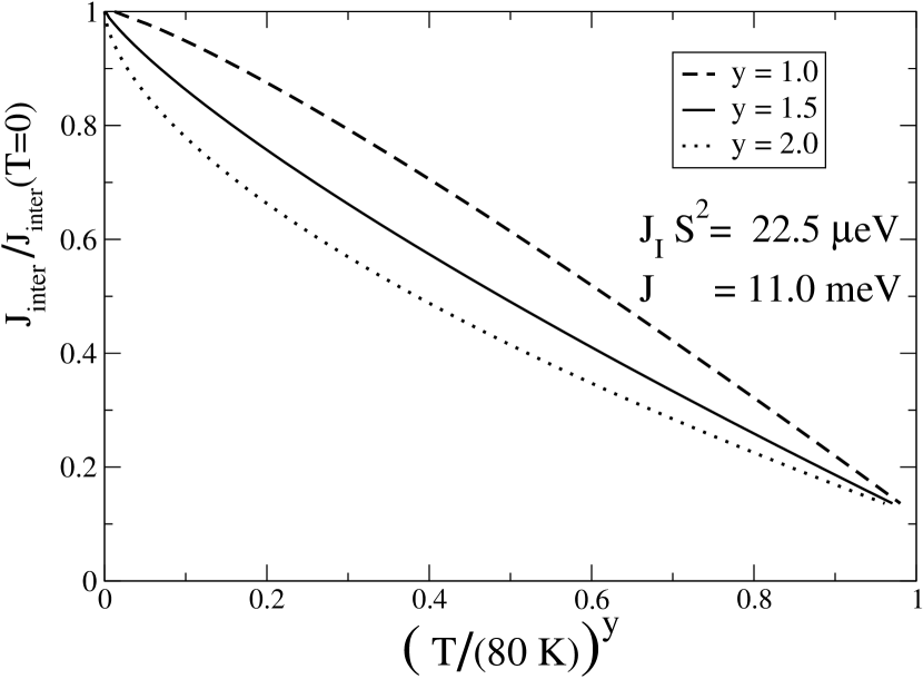
Figure 2: Temperature dependent factor of $J_{\rm inter}$ plotted against temperature in different scales. Here and in the following figures solely the magnetic contribution to the temperature dependence is shown.

This equation can be easily evaluated. Furthermore an analytical expression can be derived:
Let us assume, e.g., a quadratic lattice. The dominating terms in the sum over the two dimensional Brillouin zone stem from the vicinity of the $\Gamma$-point where $q$ is small and we can write: $J_{\mathbf{q}}\approx Jq^{2}$, where $q$ is the norm of $\mathbf{q}$. After expanding the logarithm and replacing the $\mathbf{q}$-summation by an integral we get

$$J_{\rm inter} \approx J_{I}S^{2}-k_{B}T\sum_{n=1}^{\infty}\frac{1}{n}e^{-\beta B^{\prime}n}\left(1-e^{-\beta\cdot 2J_{I}Sn}\right)\cdot$$ (21)

$$\cdot\frac{1}{2\pi}\int_{0}^{q_{0}}\,dq\,qe^{-\beta\,2JSnq^{2}}$$

The integral is written in polar coordinates $(q,\phi)$ and the trivial $\phi$ integration has already been performed. $q_{0}$ is the averaged extension of the first Brillouin zone. Since terms with large values of $q$ only contribute negligibly to the integral, we may approximately replace the upper limit by infinity and use the tabulated integral $\int_{0}^{\infty}\,dt\,te^{-\alpha t}=(2\alpha)^{-1}$. Thus we end up with

$$f(T) = \frac{J_{\rm inter}(T)}{J_{\rm inter}(0)}$$

$$= 1-\frac{1}{8\pi JS}\frac{1}{J_{\rm inter}(0)}\left(k_{B}T\right)^{2}\cdot\Sigma(T)\quad,$$

$$\Sigma(T) = \sum_{n=1}^{\infty}\frac{1}{n^{2}}e^{-\beta Bn}\left(1-e^{-\frac{1}{S}J_{\rm inter}(0)\beta n}\right)\quad.$$ (22)

The infinite sum converges by the majorant criterion (note the constraint $B^{\prime}>|2J_{I}S|$ for anti-ferromagnetic coupling). The first derivative of $\Sigma(T)$ with respect to $T$ is negativefoot1 , while the first derivative of the term $k_{B}T\cdot\Sigma(T)$ is larger than zero. Thus the coupling decreases with temperature faster than $1-x\;T$ but slower than $1-x\;T^{2}$. The effective coefficient $y$, defined in Eq. (8), is between 1 and 2. The evaluation of Eq.(20) clearly corroborates this trend as can be seen in Fig.2. The effective coefficient is around $y=1.5$ except for very low temperatures $T<30\,K$. Here and in the following calculations the parameters $J_{I}$ are chosen to be comparable with experiment LiB03 ; LiB03a using Eq.(13). The effective intra-layer coupling $J$ is chosen such that the spin wave stiffness of the bulk material has a realistic order of magnitude ($J=10-100~{}{\rm meV}$ for transition metalsPKT01 ). For this parameters we find a certain decrease of $J_{\rm inter}$ between $0$ and $300\,K$.

Figure 3: Temperature dependent factor of $J_{\rm inter}$ plotted against temperature for different zero temperature couplings $J_{I}S^{2}$.

Fig.3 shows the dependence of $f(T)$ on the zero temperature coupling $J_{\rm inter}(0)$. The temperature dependence is more pronounced if $J_{\rm inter}(0)$ is small. However, the differences between the curves are very small. $J_{\rm inter}(0)$ appears twice in Eq.(22), once in the denominator and once in the exponent. These contributions seem to cancel each other almost perfectly.
The dependence on the intralayer coupling $J$ is much more pronounced. This is seen in Eq.(22) as well as in Fig.4. Materials with a large effective coupling $J$ have a much less pronounced temperature dependence.
In addition the function $f(T)$ depends on the external field $B$ (Fig.5). External fields stabilize the coupling, since more energy is needed to excite a magnon and the ground state is stabilized.
This property also influences the dependence of $f(T)$ on the coupling sign. One can read off from Eq.(22):

$$f \big{(}T,{\rm fm},B^{\prime}-2J_{I}S\big{)}$$

$$= f \big{(}T,{\rm afm},B^{\prime}\big{)}\quad,$$ (23)

which means, that for anti-ferromagnetic coupling an effective field

$$B_{\rm eff}=B^{\prime}-2J_{I}S\quad,$$ (24)

rather than the pure external field, is decisive. Thus the temperature dependence is more pronounced for anti-ferromagnetic coupling compared with ferromagnetic coupling. This is shown in Fig.6, where results for anti-ferromagnetic and ferromagnetic coupling are shown for $|J_{\rm inter}(0)|=22.5\,\mu eV$. For comparison a curve for $J_{\rm inter}(0)=+40\,\mu eV$ is shown. The dependence on the norm of $J_{\rm inter}$ is almost negligible compared to the influence of the sign. However, this very influence is rather weak, too.

Figure 4: Temperature dependent factor of $J_{\rm inter}$ plotted against temperature for different intra-layer couplings $J$

The behavior of the magnetic contribution worked out above, will be compared to the spacer and interface contribution in the next section.

IV Comparison of the different coupling mechanisms

Figure 5: Temperature dependent factor of $J_{\rm inter}$ plotted against temperature for different external fields.

The spacer, interface and magnetic contribution show some similarities:

• In the temperature regime where the theories are applicable the functional dependencies $J_{\rm inter}(T)$ resemble each other. We have for all contributions

  $$f(T)=\frac{J_{\rm inter}(T)}{J_{\rm inter}(0)}\approx 1-x\,T^{y}\quad,$$ (25)

  with $1<y<2$.

There are, however, certain differences:

• The dependence of $f(T)$ on the spacer thickness $D$ is quite different. The spacer mechanism exhibits a strict $D\cdot T$ dependence

  $$f^{\rm spacer}(D,T)=f(D\cdot T)\quad,$$ (26)

  the interface contribution is independent of $D$,

  $$f^{\rm interface}(D,T)=f(T)\quad,$$ (27)

  while the magnetic layer contribution shows a very weak implicit dependence via the zero temperature coupling

  $$f^{\rm magnet}(D,T)=f(J_{\rm inter}(0,D),T)\quad.$$ (28)

  that oscillates with the spacer thickness.

• There are also differences concerning the dependence on the magnetic material. The spacer contribution is independent of the magnetic material, the interface contribution may be material dependent via $D_{\phi}$ and the magnetic contribution exhibits a strong $\frac{1}{J}$ dependence, where $J$ is the effective coupling between the magnetic moments of the film.

• The magnetic contribution shows a (weak) dependence on the coupling sign, i.e. the temperature dependence is more pronounced for anti-ferromagnetic interlayer coupling, if the coupling strength is the same.

• The magnetic contribution is suppressed by an external field. To our knowledge, there is no such effect for the spacer or interface contribution.

• Alloying of the spacer introduces disorder and can reduce the amplitude of the couplingDKB98 . In this case the temperature dependence of the spacer contribution is reduced (see Ref. 18), while the temperature dependence of the magnetic contribution is increased (see Fig.3). However, this statement has to be taken with care, since alloying may also change the stationary Fermi surface spanning vectors and therewith the parameters $c_{\alpha}$ of Eq.(5). For this case alloying may be increase or decrease the spacer contribution depending on the specific combination of materials.

The specific behavior of the different mechanisms opens the possibility to identify the dominant mechanism by experiments. To this end we will review existing experiments and propose new experiments in the next section.

Figure 6: Temperature dependent factor of $J_{\rm inter}$ plotted against temperature for two ferromagnetic couplings and one anti-ferromagnetic coupling.

V Experiments

There are not many reported studies dealing with the temperature dependence $f(T)$ of the interlayer coupling. Z. Zhang et.al. ZZW94a ; ZZW94 studied ${\rm Co_{\rm 32\,\AA}/Ru_{\rm x\,\AA}/Co_{\rm 32\,\AA}}$ trilayers using ferromagnetic resonance. N. Perat and A. Dina studied ${\rm Co_{\rm 24\AA}/Cu_{x\AA}/Co_{\rm 24\AA}(hcp)}$ samples using squid magnetization measurementsPeD97 . J. Lindner and K. Baberschke performed ferromagnetic resonance measurements on a ${\rm Ni_{7}/Cu_{x}/Co_{2}(001)}$ systemLiB03a .
With one exception (Ref. 19,20: $D=24\,\AA$) all data can be fitted to Eq.(5). In all cases the parameter $c$ deviates clearly from the value expected from the spacer contribution (6) alone. It was further shown by Lindner et.al.LRK02 that the data can be fitted with the same accuracy to Eq.(8) with $y=1.5$. Both functional behaviors fulfill our expectation and can be caused by any of the described mechanisms. As discussed in detail above we have to know the dependence on the intra-layer coupling $J$ or on the spacer thickness to discriminate between the different contributions. Unfortunately the dependence on the magnetic material (and therewith on $J$) was not investigated in these studies. On the other hand, there are some data describing the influence of the spacer thickness. They are summarized in Fig.7. There are two parameters that are a measure of the thickness dependence of $f(T)$, namely the parameter $x$ from Eq.(8) and the parameter $c$ from Eq.(5). Large $x$ or large $c$ indicate a large suppression of the coupling by temperature. In Fig.7 the parameter $c$ is displayed rather than $x$ since it is more convenient to obtain its values from the experimental studies. The data points were taken directly from the papers or were extracted from the respective plots.
The parameter $c$ increases with the spacer thickness $D$ in all cases. This qualitative trend is in accordance with the spacer but also with the magnetic contribution. A linear increase would favor a strong importance of the spacer contribution, while oscillations that follow $J_{\rm inter}(0,D)$ would indicate a decisive role of the magnetic mechanism. However, in all works there are not enough data points to establish a linear or oscillatory behavior.
If one assumes for a moment a linear dependence according to Eq. (6) the solid lines in Fig.7 are obtained. The graphs of Refs. 19, 20 and 21 show a certain finite value for the $D=0$ extrapolation. Thus the spacer mechanism can not be the only source of temperature dependence in these samples.

Figure 7: Parameter $c$ displayed against spacer thickness as obtained by different experiments. Large values of $c$ mean pronounced temperature dependence. The solid lines are linear extrapolations to $D=0$

The spacer thickness dependence is very weak in Ref. 21 as expected by the magnetic contribution (indeed $J_{\rm inter}(0)$ is very similar for both data points). On the other hand the value $a$ from Eq.(6), which can be read off from the slope in Fig.7, is in rather good agreement with model theory:

$$a_{\rm ex}\approx 2.4\cdot 10^{-4}\,K^{-1}\quad\quad a_{\rm th}\approx 1\cdot 10^{-4}\,K^{-1}$$ (29)

The theoretical value is taken from Ref. 2.
The situation in the ruthenium samplesZZW94a ; ZZW94 seems to be different. The contribution scaling with the spacer thickness is more important. There is a very interesting feature in the upper left panel of Fig.7. There seems to be evidence for a slight oscillatory behavior of $c$ as a function of spacer thickness. The oscillation follows the $J_{\rm inter}(0)$ value. For the spacer thicknesses of Ref. 21 no oscillations of $J_{\rm inter}(0)$with spacer thickness $D$ are found and consequently no oscillation of $c$. This behavior favors a magnetic mechanism. On the other hand the fitted $a$ value from Eq.(6) is again in reasonable agreement with the theoretical result

$$a_{\rm ex}\approx 5\cdot 10^{-4}\,K^{-1}\quad\quad a_{\rm th}\approx 2.4\cdot 10^{-4}\,K^{-1}\quad.$$ (30)

The deviations of a factor 2-3 are not alarming, since the linear fits are of course of bad quality due to the small number of data points.
The data of Ref. 15 reveal a different picture. Here the parameter $c$ really seems to scale with the spacer thickness as predicted by the model theory of the spacer contribution. Of course two points are not enough to confirm this mechanism and the value of $a$ differs from the theoretical one by an order of magnitude.

$$a_{\rm ex}\approx 2.4\cdot 10^{-3}\,K^{-1}\quad\quad a_{\rm th}\approx 1\cdot 10^{-4}\,K^{-1}\quad.$$ (31)

Again the theoretical value is taken from Ref. 2. This system was also investigated by ab-initio calculations DKB99 corroborating the order of magnitude of $a_{\rm th}$. Thus the origin of the strong difference remains unclear.
In summary, no clear conclusion can be drawn from the existing experiments. There is clearly a need for more experimental data. We propose a systematic investigation of the temperature dependence at different spacer thicknesses. The spacer thickness should be varied at least over a full oscillation of $J_{\rm inter}$ with $D$. The parameters $c$ of Eq.(5) or $x$ of Eq.(8) should be displayed as a function of spacer thickness $D$ and as a function of the zero temperature coupling $J_{\rm inter}(0)$.
In addition we propose the study of the temperature dependence for different magnetic materials (e.g. Co, Ni) separated by the same spacer (e.g. Cu).
With these experimental results at hand and with the theoretical results summarized in section 4 one may isolate the dominating mechanism that causes the temperature dependence of the interlayer coupling in metallic trilayers.
There is clearly a need for more theoretical studies as well. Both aspects, the spacer and interface contribution on the one hand and the magnetic contribution on the other, should be described in one model on equal footing. Furthermore the restriction to low temperatures, which is up to now inherent to all models, should be removed and effects as the temperature dependence of the reflection coefficients should be studied as well.

VI Summary

The reduction of the interlayer coupling with temperature in metallic multilayers may be caused by effects within the spacer, at the interface, or within the magnetic layers. We derived the magnetic part at low temperatures and discussed its dependence on the spacer layer thickness, on the magnetic materials, on the sign of the coupling, and on the external field. These dependencies were compared with those of the spacer and interface contributions. As a main result we found that the functional dependence of the temperature dependent factor $f(T)$ is roughly the same for all mechanisms. There are certain differences in the dependence of $f(T)$ on the spacer thickness and on the magnetic material. Based on these considerations we proposed experiments that are able to identify the dominant mechanism in metallic trilayers which is not possible with the experimental data available today.

References

- (1) see e.g. P. Bruno, Phys. Rev. B 52, 411 (1995)
- (2) P. Bruno and C. Chappert, Phys. Rev Lett. 67, 1602 (1991)
- (3) D. M. Edwards, J. Mathon, R. B. Muniz, and M. S. Phan, Phys. Rev Lett. 67, 493 (1991)
- (4) J. d’Albuquerque e Castro, J. Mathon, M. Villeret, and A. Umerski, Phys. Rev. B 53, R13306 (1996)
- (5) A. T. Costa, J. d’Albuquerque e Castro, M. S. Ferreira, and R. B. Muniz, Phys. Rev. B 60, 11894 (1999)
- (6) P. Bruno, Eur. Phys. J. B 11, 83 (1999)
- (7) see e.g.: J. Kudrnovsky, V. Drchal, I. Turek, P. Bruno, P. Dederichs, and P. Weinberger: ”ab-initio theory of the interlayer exchange coupling” in H. Dreysse (Ed.) Electronic Structure and Physical Properties of Solids. The Uses of the LMTO Method”,313 (Springer, Berlin 2000),cond-mat/9811152v2
- (8) V. Drchal, J. Kudrnovsky, P. Bruno, I. Turek, P. H. Dederichs, and P. Weinberger, Phys. Rev. B 60, 9588 (1999)
- (9) There is no unique conventien concerning the sign and the prefactor in this definition.
- (10) B. C. Lee and Y.-C. Chang, Phys. Rev. B 62, 3888 (2000)
- (11) J. Lindner and K. Baberschke, J. Phys.:Condens. Matter 15, R193 (2003)
- (12) N. S. Almeida, D. L. Mills, and M. Teitelman, Phys. Rev. Lett. 75, 733 (1995)
- (13) F. J. Dyson, Phys. Rev. 102, 1217 (1965)
- (14) T. Holstein and H. Primakoff, Phys. Rev. 58, 1098 (1940)
- (15) J. Lindner and K. Baberschke, J. Phys.:Condens. Matter 15, S465 (2003)
- (16) this holds only for which is usually fulfilled in experiments for
- (17) M. Pajda, J. Kudrnovsky,I. Turek, V. Drchal, and P. Bruno, Phys. Rev. B 64, 174402 (2001)
- (18) V. Drchal, J. Kudrnovsky, P. Bruno, P. H. Dederichs, and P. Weinberger, Phil. Mag. B 78, 571(1998)
- (19) Z. Zhang, L. Zhou, P. E. Wigen, and K. Ounadjela, Phys. Rev. B 50, 6094 (1994)
- (20) Z. Zhang, L. Zhou, P. E. Wigen, and K. Ounadjela, Phys. Rev. Lett. 73, 336 (1994)
- (21) N. Persat and A. Dinia, Phys. Rev. B 56, 2676 (1997)
- (22) J. Lindner, C. Rüdt, E. Kosubek, P. Poulopoulos, K. Baberschke, P. Blomquist, R. Wäppling, and D. L. Mills, Phys. Rev. Lett. 88, 167206 (2002)