Simple quantum feedback of a solid-state qubit

Abstract

We propose an experiment on quantum feedback control of a solid-state qubit, which is almost within the reach of the present-day technology. Similar to the earlier proposal, the feedback loop is used to maintain the coherent (Rabi) oscillations in a qubit for an arbitrary long time; however, this is done in a significantly simpler way, which requires much smaller bandwidth of the control circuitry. The main idea is to use the quadrature components of the noisy detector current to monitor approximately the phase of qubit oscillations. The price for simplicity is a less-than-ideal operation: the fidelity is limited by about 95%. The feedback loop operation can be experimentally verified by appearance of a positive in-phase component of the detector current relative to an external oscillating signal used for synchronization.

The needs of quantum computing [1] are fueling a rapid progress in experiments with solid-state qubits. In particular, quantum coherent (Rabi) oscillations have been demonstrated using superconducting charge, flux, and phase qubits [2] as well as double-quantum-dot qubits.[3] Successful experiments with two superconducting qubits have also been demonstrated. [4] Even though at present only very basic operations with qubits are experimentally accessible, more advanced experiments are a natural next stage. One of the directions for the advanced qubit control is realization of the quantum feedback control of a solid-state qubit, [5] which can be used in a quantum computer for qubit initialization and is also an important demonstration by itself, clarifying the controversial issue of gradual collapse of a quantum state. (In optics quantum feedback control was proposed more than a decade ago [6] and has been already demonstrated experimentally.[7])

For the analysis of a quantum feedback we have to take into account the process of continuous qubit collapse. Therefore, the conventional approach to continuous quantum measurement [8, 9] is inapplicable, and it is necessary to use the recently developed Bayesian approach [10] or the equivalent (though much different technically) approach of quantum trajectories.[11] The possibility of a quantum feedback is based on the fact that measurement by an ideal solid-state detector (with 100% quantum efficiency $\eta$) does not decohere a single qubit, [10] even though it decoheres an ensemble of qubits because each qubit evolves in a different way. The random evolution of a qubit in the process of measurement can be monitored using the noisy detector output, with accuracy depending on $\eta$, so that for an ideal detector ($\eta=1$) even the monitoring of qubit wavefunction is possible. An example of theoretically ideal solid state detector is [12, 10] the quantum point contact ($\eta$ comparable to 1 has been demonstrated experimentally [13]). The single-electron transistor is significantly nonideal [9, 10, 14] ($\eta\ll 1$) in the semiclassical “orthodox” mode of operation; [15] however, it can reach ideality in some modes based on cotunneling or Cooper pair tunneling. [16]

Monitoring of the quantum state in real time can naturally be used for continuous feedback control of a quantum system. In the experiment proposed in Ref. [5] the quantum feedback is used to maintain quantum coherent (Rabi[17]) oscillations in a qubit for an arbitrary long time, synchronizing them with an external classical signal. This is done by measuring the noisy current $I(t)$ in a weakly coupled detector and using the quantum Bayesian equations [10] to translate information contained in $I(t)$ into the evolution of qubit density matrix $\rho(t)$. After that $\rho(t)$ is compared with the desired quantum state $\rho_{d}(t)$, and the calculated difference is used to control the qubit Hamiltonian in order to decrease the difference. Notice that the measurement backaction necessarily shifts the phase of Rabi oscillations in a random way (adding it to dephasing due to environment); however, the information contained in $I(t)$ is sufficient to monitor this change and therefore restore the desired phase.

An important difficulty in such experiment is a necessity to solve the Bayesian equations in real time. Moreover, the bandwidth of the line delivering $I(t)$ to the circuit solving the Bayesian equations, should be significantly wider than the Rabi frequency $\Omega$ (otherwise the information contained in the noise is lost). Unfortunately, these conditions are unrealistic for the present-day experiments with solid-state qubits. (The “direct” feedback also analyzed in Ref. [5] does not require solving Bayesian equations, but requires a wide bandwidth of the whole feedback loop.)

In this paper we propose and analyze a much simpler way (Fig. 1) of processing the information carried by the detector current $I(t)$. The idea is to use the fact that besides noise, $I(t)$ contains an oscillating contribution due to Rabi oscillations in the measured qubit. Therefore, if we apply $I(t)$ to a simple tank circuit (which is in resonance with $\Omega$), then the phase of the tank circuit oscillations will depend on the phase of Rabi oscillations. Instead of using the tank circuit, almost equivalent theoretically procedure is to mix $I(t)$ with the signal from a local oscillator (Fig. 1) in order to determine two quadrature amplitudes of $I(t)$ at frequency $\Omega$, which will carry information on the phase of Rabi oscillations. Since diffusion of the Rabi phase is a slow process (assuming weak coupling to the detector and environment), the further circuitry can be relatively slow, limited by the qubit dephasing rate, but not limited by much higher Rabi frequency. The simplicity of the information processing and relatively small required bandwidth are the main advantages of this proposal in comparison with Ref. [5] The experiment can be realized using either superconducting [2, 4, 18] or GaAs [3, 13] technology.

The idea of this proposal partially stems from the fact that in absence of feedback the qubit Rabi oscillations lead to a noticeable peak in the spectral density $S_{I}(\omega)$ of the detector current at $\omega\approx\Omega$, with the peak-to-pedestal ratio up to 4 times [19] (somewhat similar experiments have been reported recently [20]). Since 4 is not a big number, one would expect quite inaccurate phase information carried by current quadratures and therefore poor operation of the feedback. Surprisingly, the quantum feedback operates much better than it would be expected from classical analysis.

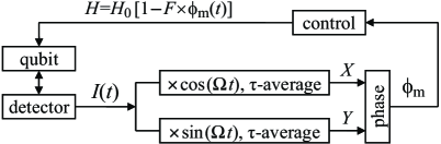
FIG. 1.: Schematic of the proposed quantum feedback loop. Two quadrature components of the detector current $I(t)$ are used to monitor approximately the phase difference between Rabi oscillations and a local oscillator, which is used to control the qubit parameter $H$. The phase can also be monitored using a tank circuit. Positive average in-phase quadrature $\langle X\rangle$ is an experimental indication of quantum feedback operation.

Let us consider a “charge” qubit (either double quantum dot or single Cooper pair box) with Hamiltonian ${\cal H}_{qb}=(\varepsilon/2)(c_{2}^{\dagger}c_{2}-c_{1}^{\dagger}c_{1})+H(c_{1}^{\dagger}c_{2}+c_{2}^{\dagger}c_{1})$, where $c_{1,2}^{\dagger}$ and $c_{1,2}$ are the creation and annihilation operators in the basis of “localized” (charge) states, $\varepsilon$ is their energy asymmetry, and the tunneling $H=H_{0}+H_{fb}(t)$ can be controlled by the feedback loop ($H_{fb}$). We assume the standard coupling [21, 10, 19] between the charge qubit and the detector (quantum point contact or single-electron transistor). Instead of writing Hamiltonians explicitly, we will characterize the measurement by two levels of the average detector current, $I_{1}$ and $I_{2}$, corresponding to the two charge states, by the detector output noise $S_{I}$, and by the total ensemble-averaged qubit dephasing rate $\Gamma$ due to detector backaction and environment. Assuming sufficiently large detector voltage and quasicontinuous detector current $I(t)$, we describe the qubit evolution by the Bayesian equations [10] (in Stratonovich form)

$$\dot{\rho}_{11}=-2H\,\mbox{Im}\,\rho_{12}+2\rho_{11}\rho_{22}[I(t)-I_{0}]\,\Delta I/S_{I},$$ (1)

$${\dot{\rho}}_{12}=i\varepsilon\rho_{12}+iH(\rho_{11}-\rho_{22})-\gamma\rho_{12}$$ (2)

$$\hskip 22.76228pt-(\rho_{11}-\rho_{22})\rho_{12}[I(t)-I_{0}]\,\Delta I/S_{I}\,,$$ (3)

where $\hbar=1$, $\Delta I=I_{1}-I_{2}$, $I_{0}=(I_{1}+I_{2})/2$, and $\gamma=\Gamma-(\Delta I)^{2}/4S_{I}$. The qubit decoherence rate $\gamma=\gamma_{d}+\gamma_{e}$ is due to detector nonideality, $\gamma_{d}=(\eta^{-1}-1)(\Delta I)^{2}/S_{I}$, and due to additional coupling with environment ($\gamma_{e}$). The current $I(t)=I_{0}+(\rho_{11}-\rho_{22})\Delta I/2+\xi(t)$ has the noise component $\xi(t)$ with the flat (white) spectral density $S_{I}$. Notice that in the case $\varepsilon=0$ (which is assumed unless mentioned otherwise), we can disregard the evolution of $\mbox{Re}\rho_{12}$ (it becomes zero at $t\gg\Gamma^{-1}$), so only two degrees of freedom are left, which may be parameterized as $\rho_{11}-\rho_{22}=P\cos(\Omega t+\phi)$ and $2\mbox{Im}\rho_{12}=P\sin(\Omega t+\phi)$, where the feedback-maintained frequency $\Omega$ (see below) is assumed to be equal (unless stated otherwise) to the bare Rabi frequency $\Omega_{0}=(4H_{0}^{2}+\varepsilon^{2})^{1/2}=2H_{0}$. Moreover, in the ideal case $\gamma=0$ the state eventually becomes pure,[10] so that $P=1$ and the evolution can be described by only one parameter $\phi(t)$.

We assume that two quadrature components of the detector current (Fig. 1) are determined as

$$X(t)=\int^{t}_{-\infty}[I(t^{\prime})-I_{0}]\cos(\Omega t^{\prime})e^{-(t-t^{\prime})/\tau}dt^{\prime}\,,$$ (4)

$$Y(t)=\int^{t}_{-\infty}[I(t^{\prime})-I_{0}]\sin(\Omega t^{\prime})e^{-(t-t^{\prime})/\tau}dt^{\prime}\,,$$ (5)

where $\Omega$ is the local oscillator frequency applied to the mixer, and $\tau$ is the averaging time constant. Similar formulas are also applicable to the case of a tank circuit with the resonant frequency $\Omega$ and quality factor $Q=\Omega\tau/2$. If the detector current would be a harmonic signal $I(t)=I_{0}+P(\Delta I/2)\cos(\Omega t+\phi_{0})$, then $\phi_{0}=-\arctan(\langle Y\rangle/\langle X\rangle)$, so it is natural to use

$$\phi_{m}(t)\equiv-\arctan(Y/X)$$ (6)

as a monitored estimate of the phase shift $\phi(t)$ between the Rabi oscillations and the local oscillator ($\langle\dots\rangle$ means averaging over time).

Let us assume $\gamma=0$ and analyze first how close is the estimate $\phi_{m}(t)$ to the actual phase $\phi(t)$ without feedback, in which case $\phi$ evolves in a diffusive manner due to detector backaction. Figure 2 shows the rms phase difference $\Delta\phi_{rms}=\langle(\phi_{m}-\phi)^{2}\rangle^{1/2}$ (solid lines) as a function of $\tau$ for several values of the dimensionless qubit-detector coupling ${\cal C}\equiv(\Delta I)^{2}/S_{I}H_{0}$, calculated numerically using Monte Carlo simulation of the measurement process.[10] At weak coupling, ${\cal C}\lesssim 1$, the curves practically coincide, and the minimum $\Delta\phi_{rms}\approx 0.44$ is achieved at $\tau\approx 4S_{I}/(\Delta I)^{2}=1/\Gamma$, which is expectable since $\Gamma$ determines the phase diffusion: [10, 11, 19] $\langle[\phi(t)-\phi(0)]^{2}\rangle/t=\Gamma$. At larger $\tau$, $\phi_{m}$ includes too much of irrelevant information from distant past, while at smaller $\tau$ the quadrature amplitudes suffer too much from the noise. At $\tau\rightarrow 0$ (as well as at $\tau\rightarrow\infty$) $\Delta\phi_{rms}\rightarrow\pi/\sqrt{3}\approx 1.81$ that corresponds to the uniform distribution of $\Delta\phi=\phi_{m}-\phi$ (complete absence of correlation between $\phi$ and $\phi_{m}$) within $\pm\pi$ interval (all phases are defined modulo $2\pi$).

It it important to notice that the calculated $\Delta\phi_{rms}$ is significantly smaller than for a naive classical case, in which the noise $\xi(t)$ is not correlated with diffusive evolution of $\phi$. The dotted line in Fig. 2 shows the result for such a case at weak coupling, which has a minimum $\Delta\phi_{rms}\approx 1.0$ [actually, for this curve we even increased the signal, assuming $I(t)-I_{0}=\sqrt{2}(\Delta I/2)\cos(\Omega t+\phi)+\xi(t)$, which corresponds to correct spectrum[19]]. Even more surprisingly, at $\tau>2.5S_{I}/(\Delta I)^{2}$ the inaccuracy $\Delta\phi_{rms}$ in the quantum case is smaller than for the classical noiseless case, $\xi(t)=0$ (dashed line), which means that the noise improves the monitoring accuracy. This quantum behavior can be understood from the phase evolution equation [5, 10]

$$\dot{\phi}=-[I(t)-I_{0}]\sin(\Omega t+\phi)(\Delta I/S_{I})+\Omega_{0}-\Omega.$$ (7)

This equation [22] shows that the quadrature component of the noise which shifts the observed phase $\phi_{m}$, also shifts the actual phase $\phi$ in the same direction. In other words, when the noise imitates oscillations, it forces the real Rabi oscillations to evolve closer to what is observed.

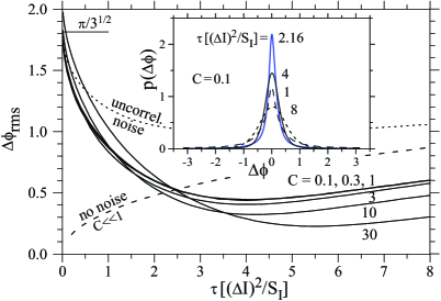
FIG. 2.: Dependence of monitoring inaccuracy $\Delta\phi_{rms}$ on averaging time $\tau$ without feedback for several values of coupling ${\cal C}$. Dashed and dotted lines correspond to classical signals. Inset: distribution of $\Delta\phi$ for several $\tau$ at weak coupling.

Inset in Fig. 2 shows the distribution of $\Delta\phi$ in the weak coupling limit for several values of $\tau$. The distributions are significantly non-Gaussian with the central part significantly narrower then $\Delta\phi_{rms}$. It is interesting that the value $\tau=4S_{I}/(\Delta I)^{2}$ corresponding to the minimum $\Delta\phi_{rms}$, does not provide the highest peak of the $\Delta\phi$ distribution. To find the best $\tau$ in this respect, let us compare the monitored phase evolution $\dot{\phi}_{m}=-[I(t)-I_{0}]\sin(\Omega t+\phi_{m})/(X^{2}+Y^{2})^{1/2}$, with Eq. (7). We would expect the best approximation of $\phi$ by $\phi_{m}$ when $\langle X^{2}+Y^{2}\rangle=(S_{I}/\Delta I)^{2}$. Using the definitions (4)–(5) and the current-current correlation function [19] $\langle I(0)I(t)\rangle=(S_{I}/2)\delta(t)+(\Delta I/2)^{2}\cos(\Omega t)\exp[-(\Delta I)^{2}t/8S_{I}]$, we obtain $\langle X^{2}+Y^{2}\rangle=S_{I}\tau[1/4+1/(1+8S_{I}/(\Delta I)^{2}\tau)]$ at $\Omega\tau\gg 1$ and ${\cal C}\ll 1$, so the condition $\langle X^{2}+Y^{2}\rangle=(S_{I}/\Delta I)^{2}$ is satisfied at $\tau(\Delta I)^{2}/S_{I}=(2/5)(\sqrt{41}-1)\approx 2.16$. This indeed corresponds to the largest peak of $\Delta\phi$ distribution (see inset in Fig. 2).

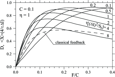
FIG. 3.: Dependence of the synchronization degree $D$ on the feedback factor $F$ in ideal case ($\gamma=0$) for several $\tau$. Experimentally $D$ can be measured via average in-phase current quadrature $\langle X\rangle$. Dashed line is for a classical feedback.

Reasonably small difference between $\phi$ and $\phi_{m}$ in absence of feedback implies that we can expect decent operation of the quantum feedback loop in which the phase estimate $\phi_{m}$ is used for determining the feedback action. Similar to Ref. [5] we consider the feedback loop, which aim is to suppress the fluctuations of the Rabi phase, so that the goal is $\phi(t)=0$ (or as small as possible). It has been shown that this goal can be fully reached using the linear feedback rule $H_{fb}(t)/H_{0}=-F\phi(t)$, which requires exact monitoring of $\phi$; here we analyze the operation of the feedback loop with $H_{fb}/H_{0}=-F\phi_{m}(t)$, where $F$ is the dimensionless feedback factor (by definition $|\phi_{m}|<\pi$).

We will characterize the performance of the feedback loop by the synchronization degree $D=\langle P(t)\cos\phi(t)\rangle=2{\cal F}-1$ where ${\cal F}=\langle\mbox{Tr}\rho(t)\rho_{d}(t)\rangle$ is fidelity and $\rho_{d}$ corresponds to the desired perfect Rabi oscillations ($P_{d}=1$, $\phi_{d}=0$). Figure 3 shows (solid lines) the dependence of $D$ on the feedback factor $F$ for several time constants $\tau$ in the case of weak coupling ${\cal C}=0.1$ and $\gamma=0$ (we normalize $F$ by ${\cal C}$, so the results practically do not depend on ${\cal C}$ for ${\cal C}\lesssim 1$). [23] One can see that each curve has a maximum, so that the “oversteering” effect at larger $F$ makes the feedback performance worse (this is in contrast to the case of Ref. [5] in which larger $F$ was always better). Somewhat unexpectedly, $\tau=1/\Gamma=4S_{I}/(\Delta I)^{2}$ is no longer an optimum, and smaller time constants are actually better. It can be shown that the feedback loop can operate even at $\tau\ll\Omega^{-1}\ll\Gamma^{-1}$; however, we are not interested in this regime because it requires a wide bandwidth of the control circuitry. Limiting ourselves to $\tau\sim S_{I}/(\Delta I)^{2}$, we see that the maximum achievable synchronization degree $D_{max}$ is about 90% (that corresponds to the fidelity ${\cal F}$ of about 95%). It is impossible to reach 100% because the monitored simple phase estimate $\phi_{m}$ is significantly different from the actual $\phi$. It is interesting to note that a very crude estimate of $D_{max}$ as $\cos(\Delta\phi_{rms})$ using $\min(\Delta\phi_{rms})\simeq 0.44$ from the analysis without feedback, works quite well, $\cos(0.44)=0.90$ (though for different $\tau$). Dashed line in Fig. 3 shows the feedback performance for a classical signal corresponding to the dotted line in Fig. 2, assuming $\tau(\Delta I)^{2}/S_{I}=1$. As expected, it operates much worse than the quantum feedback because of the reason discussed above. [The crude estimate $D_{max}\sim\cos(\Delta\phi_{rms,\min})=\cos(1.0)=0.54$ still works well.]

An important question is how the operation of the quantum feedback loop can be verified experimentally. One of the easiest ways is to check that the average value $\langle X\rangle$ of the in-phase quadrature component $X(t)$ becomes positive, while in absence of feedback ($F=0$) positive and negative values of $X$ are obviously equally probable. Notice that any Hamiltonian control of a qubit which is not based on the information obtained from the detector (i.e. feedback control) cannot provide nonzero $\langle X\rangle$. [24] It is easy to show that $\langle X\rangle=[D+\langle P\cos(2\Omega_{m}+\phi)\rangle]\tau\Delta I/4$, and since the second term in brackets vanishes at weak coupling (and $\varepsilon=0$), therefore $\langle X\rangle$ is directly related to $D$. The numerical results for $\langle X\rangle/(\tau\Delta I/4)$ practically coincide with the curves for $D$ in Fig. 3 (within the thickness of the line).

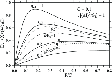
FIG. 4.: Solid lines: synchronization degree $D$ (and in-phase current quadrature $\langle X\rangle$) as functions of $F$ for several values of the detection efficiency $\eta_{eff}$. Dashed and dotted lines illustrate the effects of the energy mismatch ($\varepsilon\neq 0$) and the frequency mismatch ($\Omega\neq\Omega_{0}$).

The ideal case $\gamma=0$ is obviously not realizable in an experiment because of finite nonideality of a detector ($\eta<1$) and presence of an extra environment ($\gamma_{e}>0$). Both effects can be taken into account simultaneously introducing effective efficiency of quantum detection $\eta_{eff}=[\eta^{-1}+\gamma_{e}S_{I}/(\Delta I)^{2}]^{-1}$. Figure 4 shows (solid lines) the feedback performance for several values of $\eta_{eff}$ assuming $\tau(\Delta I)^{2}/S_{I}=1$. One can see that $\eta_{eff}\sim 0.1$ is still a sufficient value for a noticeable operation of the quantum feedback loop. Notice that $D_{max}$ is limited at least by the state purity, $D_{max}<P$, which is [22] $P\approx\sqrt{2\eta_{eff}}$ at $\eta_{eff}\ll 1$ and ${\cal C}/\eta\ll 1$ ($D_{max}=P$ can be reached by the feedback of Ref. [5] but not by the feedback studied here).

Finally, let us discuss how accurately the conditions $\Omega=\Omega_{0}$ and $\varepsilon=0$ should be satisfied in an experiment. If $\Omega$ is different from $\Omega_{0}$, then without feedback the phase $\phi$ linearly grows in time [Eq. (7)]. However, if the feedback loop operation is faster than $|\Delta\Omega|=|\Omega-\Omega_{0}|$, the linear growth of $\phi$ is stopped by adjusting the Rabi frequency $\Omega_{0}$ to match the desired frequency $\Omega$. Dotted lines in Fig. 4 show the feedback operation for $\eta_{eff}=0.2$ and two values of $\Delta\Omega$, confirming still good operation at $|\Delta\Omega|\ll{\cal C}\Omega\sim\Gamma\sim\tau^{-1}$. Notice that the frequency mismatch leads to nonzero $\langle\phi_{m}\rangle$ and therefore can be noticed and corrected. Energy mismatch ($\varepsilon\neq 0$) also worsens the performance of the feedback loop; however, the dashed lines in Fig. 4 ($\eta_{eff}=0.5$) show that a relatively large mismatch ($\varepsilon\lesssim H_{0}$) can be tolerated.

In conclusion, we have proposed and analyzed the quantum feedback loop for a solid-state qubit, based on monitoring the phase of Rabi oscillations via quadrature components of the current in a weakly coupled detector. Surprisingly, it operates much better than one could guess from relatively small spectral peak of the detector output in absence of feedback. The work was supported by NSA and ARDA under ARO grant DAAD19-01-1-0491.

REFERENCES

- [1] M. A. Nielsen and I. L. Chuang, Quantum computation and quantum information (Cambridge University Press, Cambridge, 2000).
- [2] Y. Nakamura et al., Nature 398, 786 (1999); D. Vion et al., Science 296, 886 (2002); Duty et al., Phys. Rev. B 69, 140503 (2004); A. Guillaume et al., cond-mat/0312544; I. Chiorescu et al., Science 299, 1869 (2003); J. M. Martinis et al., Phys. Rev. Lett. 90 , 117901 (2002).
- [3] T. Hayashi et al., Phys. Rev. Lett. 91, 226804 (2003).
- [4] Yu. A. Pashkin et al., Nature 42, 823 (2003); A. J. Berkley et al., Science 300, 1548 (2003).
- [5] R. Ruskov and A. N. Korotkov, Phys. Rev. B 66, 041401 (2002).
- [6] H. M. Wiseman and G. J. Milburn, Phys. Rev. Lett. 70, 548 (1993).
- [7] M. A. Armen et al., Phys. Rev. Lett. 89, 133602 (2002); JM Geremia et al., quant-ph/0401107.
- [8] A. O. Caldeira and A. J. Leggett, Ann. Phys. (N.Y.) 149, 374 (1983); W. H. Zurek, Phys. Today, 44 (10), 36 (1991).
- [9] Y. Makhlin, G. Schön, and A. Shnirman, Rev. Mod. Phys. 73, 357 (2001).
- [10] A. N. Korotkov, Phys. Rev. B 60, 5737 (1999); Phys. Rev. B 63, 115403 (2001); cond-mat/0209629; Phys. Rev. B 67 235408 (2003); W. Mao et al., cond-mat/0401484.
- [11] H.-S. Goan, G. J. Milburn, H. M. Wiseman, and H. B. Sun, Phys. Rev. B 63, 125326 (2001); H.-S. Goan and G. J. Milburn, Phys. Rev. B 64, 235307 (2001); N. P. Oxtoby, H. B. Sun, and H. M. Wiseman, J. Phys.-Condens. Mat. 15, 8055 (2003).
- [12] I. L. Aleiner et al., Phys. Rev. Lett. 79, 3740 (1997).
- [13] E. Buks et al., Nature 391, 871 (1998).
- [14] M. H. Devoret and R. J. Schoelkopf, Nature 406, 1039 (2000).
- [15] D. V. Averin and K. K. Likharev, J. Low Temp. Phys. 62, 345 (1986).
- [16] A.B. Zorin, Phys. Rev. Lett. 76, 4408 (1996); A.M. van den Brink, Europhys. Lett. 58, 562 (2002); D. V. Averin, cond-mat/0010052; A. A. Clerk, S. M. Girvin. A. K. Nguyen, and A. D. Stone, Phys. Rev. Lett. 89, 176804 (2002).
- [17] We use the term “Rabi oscillations” for evolution of a qubit which state is not an energy eigenstate, not implying an rf field presence.
- [18] M. D. LaHaye et al., Nature 304, 74 (2004).
- [19] A. N. Korotkov and D. V. Averin, Phys. Rev. B 64, 165310 (2001); A. N. Korotkov, Phys. Rev. B 63, 085312 (2001); R. Ruskov and A. N. Korotkov, Phys. Rev. B 67, 075303 (2003); A. Shnirman, D. Mozyrsky, and I. Martin, cond-mat/0311325.
- [20] C. Durkan et al., Appl. Phys. Lett. 80, 458 (2002); E. Il’ichev et al., Phys. Rev. Lett. 91, 097906 (2004).
- [21] S. A. Gurvitz, Phys. Rev. B 56, 15215 (1997).
- [22] At finite (assuming and ) the phase equation is . At the last term can be neglected and state purity is given by . In particular, at .
- [23] Notice that because and , so the feedback requires only a weak change of the tunnel barrier between the qubit states.
- [24] Some procedures which include periodic dissipation phase (nonunitary operation) can be used to achieve nonzero , though much less efficiently than by the quantum feedback.