Third order correction to localization in a two-level driven system

Abstract

A general result is presented on the lack of second order corrections and on the form of the leading order Floquet quasi-energies in the high-frequency approximation for a two-level driven system. Then, by a perturbative approach in the high-frequency approximation that uses dual Dyson series and renormalization group techniques [M. Frasca, Phys. Rev. B 68, 165315 (2003)], we obtain a third order correction for a sinusoidal driving field that is the same obtained by Barata and Wreszinski [Phys. Rev. Lett. 84, 2112 (2000)], confirming their result that localization deviates from the zeros of the zero-th order Bessel function when higher order terms are taken into account. Three different expressions for this correction are compared. An important consequence of this result is that gives complete support to the correctness of both methods. Finally, the limitation of high-frequency approximations is presented by comparison with numerical results for a sinusoidal driving field.

In a recent paper by Barata and Wreszinski (BW)bw a new method to solve perturbatively the driven two-level system was presented. These authors showed that a third order correction, for the case of a sinusoidal driving field, appears to change the leading order Floquet quasi energies, in the limit of large frequency, in such a way to modify the naive result that one has localization in the two-level system at the zeros of the zero-th order Bessel function.

This analytical result is in agreement, to a certain extent as we will see, with a work by Creffield about the crossing manifolds of the localization points in this model cc1 ; cc2 . A different work by Platero, Brandes and Aguado pab showed that analytical and numerical results agree fairly well taking into account the result by Barata and Wreszinski.

The question of higher order corrections is a relevant one in view of the needs of workable two-level systems to be manipulated as qubit in quantum computers. This means that general results are important to know the proper way to drive a two-level system for such aims.

In this paper we present a several results on higher order corrections to Floquet quasi-energies for a driven two-level system. The approach we use has been already presented in fra1 . The method given there uses the dual Dyson series and renormalization group techniques. We improve the computations till third order showing equivalence with the method of Barata and Wreszinski giving in this way fully support to both methods in the high-frequency approximation.

A two-level driven system that is generally considered to implement a qubit by a solid state device has the form:

$$H=\frac{\Delta}{2}\sigma_{3}+g\sigma_{1}f(t)$$ (1)

being $\Delta$ the separation between the two levels, $g$ the coupling constant and $f(t)=f(t+T)$ a periodical driving field with period $T$ and $\omega=2\pi/T$ and $\sigma_{1}$,$\sigma_{3}$ Pauli matrices. The high-frequency regime is identified by the condition $\frac{\Delta}{\omega}\ll 1$. Floquet theory can be applied and from this we know that localization appears at the crossing of the quasi-energies hg . Then, a proper choice of the parameters can permit to drive a qubit. The other crucial parameter for our aims is $z=2g/\omega$ that we will use in the following.

We can prove a general result on the model (1) using the method of dual Dyson series given in Ref.fra1 . We introduce the unitary transformation

$$U_{F}=\exp\left[-ig\sigma_{1}\int_{0}^{t}dt^{\prime}f(t^{\prime})\right]$$ (2)

that gives the transformed Hamiltonian

$$H_{F}=\frac{\Delta}{2}\sigma_{3}\exp\left[-2gi\sigma_{1}\int_{0}^{t}dt^{\prime}f(t^{\prime})\right].$$ (3)

By introducing the Fourier series

$$\exp\left[-2gi\sigma_{1}\int_{0}^{t}dt^{\prime}f(t^{\prime})\right]=\sum_{n=-\infty}^{+\infty}c_{n}(z)e^{-in\omega t\sigma_{1}}$$ (4)

being

$$c_{n}(z)=\frac{1}{T}\int_{0}^{T}\exp\left[-in\omega t\sigma_{1}-2gi\sigma_{1}\int_{0}^{t}dt^{\prime}f(t^{\prime})\right]$$ (5)

where $\sigma_{1}$ can be treated as a c-number, it is not difficult to write down the Hamiltonian (3) in the form

$$H_{F}=H_{F0}+\sigma_{3}\sum_{n\neq 0}a_{n}(z)e^{-in\omega t\sigma_{1}}+\sigma_{2}\sum_{n\neq 0}b_{n}(z)e^{-in\omega t\sigma_{1}},$$ (6)

being $H_{F0}=\sigma_{3}a_{0}(z)+\sigma_{2}b_{0}(z)=\sigma_{3}c_{0}(z)$ the leading order Hamiltonian whose eigenvalues give the leading order Floquet quasi-energies. This expression is obtained by considering that the coefficients of the Fouries series depend on $\sigma_{1}$. Then, we are able to derive an estimation of the Floquet quasi-energies through eq.(5) for any kind of driven two-level model.

We can extend the above result by computing the second-order correction to the quasi-energies by the method of dual Dyson series fra1 . The computation with Hamiltonian (6) is quite straightforward giving the following secular contribution to the unitary evolution

$$U_{F}^{sec}(t,t_{0})=-i[\sigma_{3}a_{0}(z)+\sigma_{2}b_{0}(z)](t-t_{0})+i\sigma_{1}\sum_{n\neq 0}\frac{a_{n}^{2}(z)+b_{n}^{2}(z)}{n\omega}(t-t_{0})+\cdots$$ (7)

where we can recognize that a second order correction cannot appear when $a_{n}=\pm a_{-n}$ and $b_{n}=\pm b_{-n}$. This is precisely the case for a sinusoidal driving field having $c_{n}(z)=J_{n}(z)$ being $J_{n}(z)$ the Bessel functions of integer order. This means that eq.(29) and eq.(30) in Ref.fra1 have not the second order correction and should be corrected by eliminating it. The same is true for a square wave driving fieldcc1 ; cc2 $f(t)=\Theta(t)-2\Theta(t-T/2)$ in the interval $0\leq t<T$. In this case we have the Fourier coefficients

$$c_{n}(z)=\frac{z}{\pi}\left[\frac{\sin\pi z}{z^{2}-n^{2}}+i\sigma_{1}\frac{(-1)^{n}\cos\pi z-1}{z^{2}-n^{2}}\right]$$ (8)

and the leading order Hamiltonian $H_{F0}=\epsilon\left(\sigma_{3}\cos(\pi z/2)+\sigma_{1}\sin(\pi z/2)\right)$, being $\epsilon=\frac{\Delta}{\pi z}\sin(\pi z/2)$ and $\pm\epsilon$ the leading order Floquet quasi-energies.

A sinusoidal driving field has $f(t)=\cos(\omega t)$. Floquet theory hg gives localization, as a first approximation, for $J_{0}(z)=0$. One may ask if this result is true at any order or just as a first order approximation. Barata and Wreszinski obtained that a third order correction given by

$$BW(z)=-\frac{\Delta^{3}}{4\omega^{2}}\sum_{n_{1},n_{2}}\frac{J_{2n_{1}+1}(z)J_{2n_{2}+1}(z)J_{-2(n_{1}+n_{2}+1)}(z)}{(2n_{1}+1)(2n_{2}+1)}$$ (9)

that is not generally zero at the zeros of $J_{0}(z)$. In a successive work Barata and Cortez bc proved that the same correction could be written as

$$BC(z)=-\frac{\Delta^{3}}{4\omega^{2}}\sum_{n_{1}\neq 0,n_{2}\neq 0}\frac{J_{n_{1}}(z)J_{n_{1}-n_{2}}(z)J_{n_{2}}(z)}{n_{1}n_{2}}.$$ (10)

Our method given in Ref.fra1 needs the computation of the third order term of the unitary evolution by dual Dyson series

$$T_{3}=i\frac{\Delta^{3}}{8}\sigma_{z}\int_{t_{0}}^{t}dt_{1}\int_{t_{0}}^{t_{1}}dt_{2}\int_{t_{0}}^{t_{2}}dt_{3}\sum_{m}\sum_{n}\sum_{p}J_{m}(z)J_{n}(z)J_{p}(z)e^{-i\omega\sigma_{x}(mt_{1}-nt_{2}+pt_{3})}$$ (11)

starting from a generic initial time $t_{0}$ and being $J_{n}$ Bessel functions of integer order. Without repeating all the procedure here, our approach gives the third order correction

$$F(z)=-\frac{\Delta^{3}J_{0}(z)}{4\omega^{2}}\sum_{n\neq 0}\frac{J_{n}^{2}(z)}{n^{2}}-\frac{\Delta^{3}}{8\omega^{2}}\sum_{n_{1}\neq 0,n_{2}\neq 0,n_{1}\neq-n_{2}}\frac{J_{n_{1}}(z)J_{n_{1}+n_{2}}(z)J_{n_{2}}(z)}{n_{1}n_{2}}.$$ (12)

that yields the complete term with respect to eq.(31) in Ref.fra1 . We have given explicitly the first term with $J_{0}(z)$ that recovers the small $z$ limit. This limit is recovered by all the expressions $BW(z)$, $BC(z)$ and $F(z)$ as it should be. As already pointed out by Barata and Cortez bc , it is not possible to prove directly equivalence of this formulas by analytical means. The relationship does not depend on the properties of the Bessel functions. So, we need to content ourselves of a direct numerical check here.

In fig.1 we have compared the three expressions above, normalized by the factor $\frac{\Delta^{3}J_{0}(z)}{4\omega^{2}}$ and the result is absolutely satisfactory.

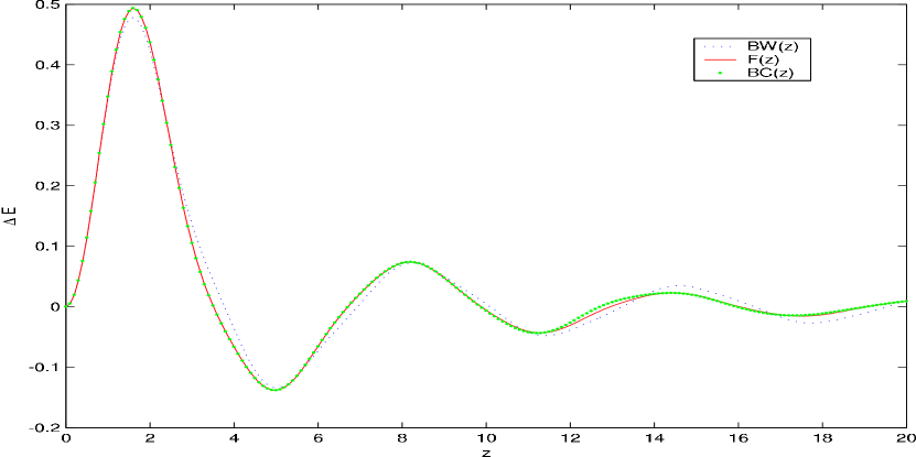
Figure 1: (Color online) The three terms, normalized by the factor $\frac{\Delta^{3}J_{0}(z)}{4\omega^{2}}$, are given here in red (solid) for $F(z)$, green (points) for $BC(z)$ and blue (dotted) for $BW(z)$. The red and green curves are almost identical.

So, the BW method and our method give both the same result supporting each other with respect to correctness as should be expected. To use one or the other becomes just a matter of taste. The fact that two different analytical approaches, in the limit of large frequency, give the same result permits us to conclude that, also by this way, it is definitely proved that zeros of $J_{0}(z)$ are just approximately localization points .

One may ask how far this third order corrections can be pushed in the ratio $\Delta/\omega$. More generally, it is rather interesting to understand the limitations of such computations. The answer can be obtained from fig.(2)

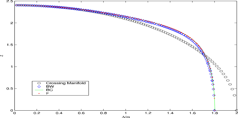
Figure 2: (Color online) The three terms, $F$ in red (dotted), $BC$ in green (solid) and $BW$ in blue (diamonds) are compared with the numerical results on crossing manifolds in black (circles) given in Ref.cc1 .

where is seen that for values of the ratio $\Delta/\omega\approx 0.5$ all the high-frequency approximations begin to fail demanding for higher order terms.

In order to give a proper picture of the problems encountered in Ref.fra1 we note as the series we obtained in it for the Floquet quasi-energies till third order was not correct [eqs.(29),(30) and (31) in Ref.fra1 ]. Rather we have shown here that no second order correction appears and that the third order correction deviates from the naive leading order result of localization at the zeros of the zero-th order Bessel function. These corrections make our approach completely equivalent, for the results, to the method conceived by Barata and Wreszinski bw . It should be said that our method makes the computation of Floquet eigenstates and quasi-energies a completely algorithmic matter, relying all the calculations on a very simple recipe.

In conclusion we have given general results for a driven two-level model giving a method to compute high-frequency leading order Floquet quasi-energies. Besides, we have proved fully equivalence between Barata and Wreszinski and our method to compute a high-frequency perturbation series. Finally, the limitation of these methods has been pointed out by comparing them with a numerical computation.

- (1) J. C. A. Barata, and W. F. Wreszinski, Phys. Rev. Lett. 84, 2112 (2000).
- (2) C. E. Creffield, Phys. Rev. B 67, 165301 (2003).
- (3) C. E. Creffield, Europhys. Lett., 66, 631 (2004).
- (4) T. Brandes, R. Aguado and G. Platero, Phys. Rev. B 69, 205326 (2004).
- (5) M. Frasca, Phys. Rev. B 68, 165315 (2003).
- (6) M. Grifoni and P. Hänggi, Phys. Rep. 304, 229 (1998).
- (7) J. C. A. Barata, D. A. Cortez, J. Math. Phys. 44, 1937 (2003); for a more complete treatment see also math-ph/0201008 (unpublished).