Option pricing with fractional volatility

Abstract

Based on empirical market data, a stochastic volatility model is proposed with volatility driven by fractional noise. The model is used to obtain a risk-neutrality option pricing formula and an option pricing equation.

Keywords: Option pricing, Stochastic volatility, Fractional noise

1 Introduction

The Black-Scholes (B-S) [1] [2] pricing formula for call options is widely used by market agents. However, rather than as a predictive formula, it is used as a means of quoting option prices in terms of another parameter, the implied volatility. If $C_{BS}\left(S_{t},K,T-t,\sigma_{t}\right)$ is the Black-Scholes price for an option at time $t$, with strike price $K$, maturity time $T$ and underlying price $S_{t}$ then, the implied volatility $\sigma_{t}^{\mathnormal{imp}}$ is such that

$$C_{BS}\left(S_{t},K,T-t,\sigma_{t}^{\mathnormal{imp}}\right)=C_{t}\left(K,T\right)$$ (1)

$C_{t}\left(K,T\right)$ being the market price of a (liquid) option.

B-S is based on unrealistic assumptions about the market process: geometric Brownian motion with constant non-stochastic volatility, continuous adjustment of the portfolio and no transaction fees. Nevertheless B-S owes its great popularity to its simplicity and to the fact that $C_{BS}$ is an invertible map from $\left[0,\infty\right)$ to $\left[0,S_{t}-Ke^{-r\left(T-t\right)}\right)$, $r$ being the risk-free rate.

The empirical shortcomings of B-S originated a vast amount of alternative models [3] $-$ [9], which attempt to explain the deviations from B-S by introducing additional degrees of freedom. The majority of these models have no compact closed-form solution and numerical solutions most often do not reproduce correctly the data profiles [10] [11].

Given the success of the Black-Scholes formula as a compact invertible parametrization, any alternative model that attempts to introduce a higher degree of market realism should, at least, provide also a compact closed-form recipe to parametrize the data.

In liquid markets the autocorrelation of price changes decays to negligible quantities in a few minutes, consistent with the absence of long term statistical arbitrage. Geometric Brownian motion models well this lack of memory, although it does not reproduce the empirical leptokurtosis. On the other hand, nonlinear functions of the returns exhibit significant positive autocorrelation. For example, there is volatility clustering, with large returns expected to be followed by large returns and small returns by small returns (of either sign). This has the clear implication that, on stochastic volatility models, long memory effects should be represented in the volatility process.

Two-factor models with one persistent factor and one quickly mean-reverting factor [12], multicomponent GARCH models as the one proposed in [13] (LM(q)-ARCH) or fractionally integrated processes [14] [15] provide adequate fits to the empirical volatility data. However, these models do not possess the analytical properties required to construct an option pricing equation generalizing Black-Scholes.

Because the market process, as well as some functionals of their variables, display approximate self-similar properties, mathematical simplicity suggests to look for descriptions in terms of fractional Brownian motion. In fact, if a nondegenerate process $X_{t}$ has finite variance, stationary increments and is self-similar

$$\mathnormal{Law}\left(X_{at}\right)=\mathnormal{Law}\left(a^{H}X_{t}\right)$$ (2)

then [16] $0<H\leq 1$ and

$$\mathnormal{Cov}\left(X_{s},X_{t}\right)=\frac{1}{2}\left(\left|s\right|^{2H}+\left|t\right|^{2H}-\left|s-t\right|^{2H}\right)E\left(X_{1}^{2}\right)$$ (3)

The simplest process with these properties is a Gaussian process called fractional Brownian motion. Fractional Brownian motion [17]

$$\mathbb{E}\left[B_{H}\left(t\right)\right]=0\qquad\mathbb{E}\left[B_{H}\left(t\right)B_{H}\left(s\right)\right]=\frac{1}{2}\left\{\left|t\right|^{2H}+\left|s\right|^{2H}-\left|t-s\right|^{2H}\right\}$$ (4)

has for $H>\frac{1}{2}$ a long range dependence

$$\sum_{n=1}^{\infty}\mathnormal{Cov}\left(B_{H}\left(1\right),B_{H}\left(n+1\right)-B_{H}\left(n\right)\right)=\infty$$ (5)

and was suggested in the past as a tool for modeling in Finance [18]. However, because it was pointed out [19] that markets based on $B_{H}\left(t\right)$ could have arbitrage, fractional Brownian motion was no longer considered, by many, as promising for mathematical modeling in Finance. The arbitrage result in [19] is a consequence of using pathwise integration. With a different definition [21],

$$\int_{a}^{b}f\left(t,\omega\right)dB_{H}\left(t\right)=\lim_{\left|\Delta\right|\rightarrow 0}\sum_{k}f\left(t_{k},\omega\right)\diamond\left(B_{H}\left(t_{k+1}\right)-B_{H}\left(t_{k}\right)\right)$$ (6)

where $\Delta:a=t_{0}<t_{1}<\cdots<t_{n}=b$ is a partition of the interval $[a,b]$, $\left|\Delta\right|=\max_{0\leq k\leq n-1}\left(t_{k+1}-t_{k}\right)$ and $\diamond$ denotes the Wick product, the integral has zero expectation value and the arbitrage result is no longer true. This is, in fact, the most natural definition because it is the Wick product that is associated to integrals of Itô type, whereas the usual product is natural for integrals of Stratonovich type.

An essentially equivalent approach constructs the stochastic integral through the divergence operator and Malliavin calculus [22]. A fully consistent stochastic calculus has therefore been developed for fractional Brownian motion [20] [21] [23] [24] [22] [25]. We will draw on these results, in particular on the fractional generalization of the Itô formula, to derive our stochastic differential market model and option pricing equation.

However, to simply postulate that the price process follows a stochastic law

$$\begin{array}[]{lll}dS_{t}&=&\mu S_{t}dt+\sigma S_{t}dB_{H}\left(t\right)\end{array}$$ (7)

with $B_{H}\left(t\right)$ ($H>1/2$) a persistent fractional Brownian motion, as done in [26] [27], although mathematically pleasant, is not phenomenological correct in view of the fact that price changes have a short memory. The simplest alternative would be to generalize current stochastic volatility models by changing the Hurst coefficient of the volatility process, namely

$$\begin{array}[]{lll}dS_{t}&=&\mu S_{t}dt+\sigma_{t}S_{t}dB\left(t\right)\\ d\sigma_{t}&=&\mu_{V}\left(\theta-\sigma_{t}\right)dt+\sigma_{V}\sigma_{t}dB_{H}\left(t\right)\end{array}$$ (8)

The price would follow a geometrical Brownian process, whereas the volatility would have a mean-reverting deterministic term and a stochastic component modeled by a geometrical fractional Brownian motion of Hurst coefficient $H>\frac{1}{2}$. This, on the one hand, would introduce a memory component on the volatility (where the data says it should be) and, on the other hand, as it is known [29] [30] stochastic volatility changes the effective probability distribution function of $S_{t}$ (even for $H=\frac{1}{2}$), generating fat tails closer to the empirical data.

However, the stochastic volatility model of Eqs.(8), as we will see later, turns out not to be justified as well, because its scaling properties are very different from those of the empirical data. For this reason we have made a detailed analysis of the data, reported in Section 2, trying to infer a model which is, at the same time, mathematically manageable and not grossly disproved by the data. Our conclusion is the following coupled stochastic system

$$\begin{array}[]{lll}dS_{t}&=&\mu S_{t}dt+\sigma_{t}S_{t}dB\left(t\right)\\ \log\sigma_{t}&=&\beta+\frac{k}{\delta}\left\{B_{H}\left(t\right)-B_{H}\left(t-\delta\right)\right\}\end{array}$$ (9)

It means that, in addition to a mean value, volatility is driven not by fractional Brownian motion but by fractional noise. Notice that our empirically based model is quite different from the usual stochastic volatility models which assume the volatility to follow an arithmetic or geometric Brownian process. $\delta$ is the observation scale of the process. In the $\delta\rightarrow 0$ limit the driving process would be the distribution-valued process $W_{H}$

$$W_{H}=\lim_{\delta\rightarrow 0}\frac{1}{\delta}\left(B_{H}\left(t\right)-B_{H}\left(t-\delta\right)\right)$$ (10)

In (9) the constant $k$ measures the strength of the volatility randomness. Although phenomenologically grounded and mathematically well specified, the stochastic system (9) is still a limited model because, in particular, the fact that the volatility is not correlated with the price process excludes the modeling of leverage effects.

In Section 3, following a risk-neutrality approach [4] [7], we use the conditional probability distributions following from Eqs.(9) to derive an option price formula and compare it with Black-Scholes, namely in terms of the equivalent implied volatility surfaces.

The risk-neutrality approach of Section 3 provides a fairly simple explicit generalization of Black-Scholes, which we believe to be based in a more realistic mathematical representation of the market process. Nevertheless it relies on some approximations which may or may not be justified. Therefore, for future reference, we derive in Section 4 an option pricing equation of wider generality and obtain an integral representation of its solution.

2 The volatility process. An empirical analysis

Option pricing being our primary motivation, the relevant time scales and temporal horizon is greater than one day. Therefore we will use daily data from the New York Stock Exchange (NYSE), the aggregate index and individual companies as well. To discount trend effects and approach asymptotic stationarity of the processes, we have detrended and rescaled the data as explained in Ref.[31].

The first objective is to check whether the assumption that the price process follows a geometric Brownian process

$$dS_{t}=S_{t}\left(\mu dt+\sigma dB_{t}\right)$$ (11)

is an acceptable hypothesis for the daily data. For detrended data $\mu=0$ and if the stochastic part is a self-similar process it should satisfy

$$E\left|\frac{S\left(t+\Delta\right)-S\left(t\right)}{S\left(t\right)}\right|\sim\Delta^{H}$$ (12)

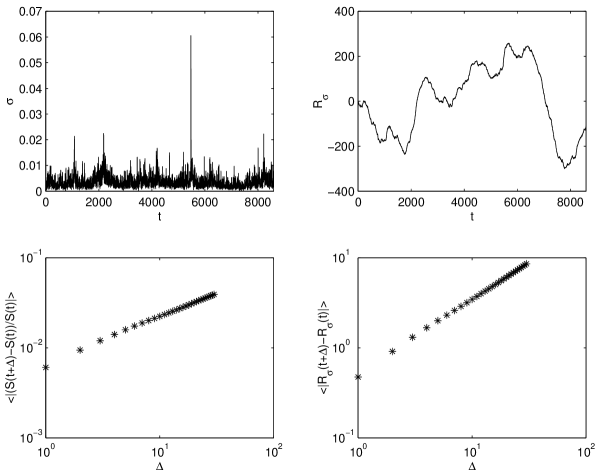
Figure 1: Self-similar properties of the price $S\left(t\right)$ and integrated log-volatility $\beta t+R_{\sigma}\left(t\right)$ processes

In the lower left panel of Fig.1 one checks Eq.(12) for the NYSE index in the period 1966$-$2000 with $\Delta=1:30$ days. We obtain approximate linearity in the log-log plot with $H=0.52$. There is a small deviation from linearity for the first few days, but one should notice that stochastic volatility effects have not yet been taken into account. So, the geometric Brownian hypothesis for the daily price process is, at least, not very unreasonable. It would imply that, in first approximation, the probability distribution would be log-normal with volatility (variance) given by

$$\sigma_{t}^{2}=\frac{1}{\left|T_{0}-T_{1}\right|}\mathnormal{var}\left(\log S_{t}\right)$$ (13)

Eq.(13) is used to extract the volatility process $\sigma_{t}$ from the data and one checks whether a relation of the form

$$E\left|\sigma\left(t+\Delta\right)-\sigma\left(t\right)\right|\sim\Delta^{H}$$ (14)

or

$$E\left|\frac{\sigma\left(t+\Delta\right)-\sigma\left(t\right)}{\sigma\left(t\right)}\right|\sim\Delta^{H}$$ (15)

hold for the volatility process. This would be the behavior implied by most of the stochastic volatility models that have been proposed in the past. It turns out that the data shows this to be a very bad hypothesis, meaning that the volatility process itself is not self-similar. However, the integrated log-volatility is well represented by a relation of the form

$$\sum_{n=0}^{t/\delta}\log\sigma\left(n\delta\right)=\beta t+R_{\sigma}\left(t\right)$$ (16)

As shown in the lower right panel of Fig.1 the $R_{\sigma}\left(t\right)$ process has self-similar properties. We will identify it with a fractional Brownian motion with Hurst coefficient $H\simeq 0.8$ (for the NYSE index),

$$R_{\sigma}\left(t\right)=kB_{H}\left(t\right)$$ (17)

The same parametrization holds for the data of all individual companies that we tested, with $H$ in the range $0.8-0.9$. This analysis bears some resemblance to the detrended fluctuation analysis technique [32]. Notice however that here, because we are using market data that has already been detrended and rescaled, it is used merely to extract the mean volatility.

Eq.(16) provides a simple mathematical representation of the volatility memory effects. In particular, it means that the volatility is not driven by fractional Brownian motion but by fractional noise,

$$\log\sigma_{t}=\beta+\frac{k}{\delta}\left(B_{H}\left(t\right)-B_{H}\left(t-\delta\right)\right)$$ (18)

$\delta$ being the observation time scale (one day, for daily data). This provides a simple interpretation of the fact that empirical return statistics depend on the observation time scale. In the $\delta\rightarrow 0$ limit (continuous time resolution) the driving process would be the distribution valued process (fractional white noise)

$$W_{H}\left(t\right)=\lim_{\delta\rightarrow 0}\frac{1}{\delta}\left(B_{H}\left(t\right)-B_{H}\left(t-\delta\right)\right)$$ (19)

For the volatility (at resolution $\delta$)

$$\sigma\left(t\right)=\theta e^{\frac{k}{\delta}\left\{B_{H}\left(t\right)-B_{H}\left(t-\delta\right)\right\}-\frac{1}{2}\left(\frac{k}{\delta}\right)^{2}\delta^{2H}}$$ (20)

the term $-\frac{1}{2}\left(\frac{k}{\delta}\right)^{2}\delta^{2H}$ being included to insure that $E\left(\sigma\left(t\right)\right)=\theta$.

Eqs. (11) and (18), or equivalently (11) and (20), define our stochastic volatility model.

This stochastic volatility model will be used in the next section to derive an option pricing formula. However it is also useful to compute the modifications implied by the stochastic volatility on the probability distribution of the price returns. From (18) one concludes that $\log\sigma_{t}$ is a Gaussian process with mean $\beta$ and covariance

$$\psi\left(s,u\right)=\frac{k^{2}}{2\delta^{2}}\left\{\left|s-u+\delta\right|^{2H}+\left|u-s+\delta\right|^{2H}-2\left|s-u\right|^{2H}\right\}$$ (21)

This Gaussian process has non-trivial correlation for $H\neq\frac{1}{2}$. At each fixed time $\log\sigma_{t}$ is a Gaussian random variable with mean $\beta$ and variance $k^{2}\delta^{2H-2}$. Then,

$$p_{\delta}\left(\sigma\right)=\frac{1}{\sigma}p_{\delta}\left(\log\sigma\right)=\frac{1}{\sqrt{2\pi}\sigma k\delta^{H-1}}\exp\left\{-\frac{\left(\log\sigma-\beta\right)^{2}}{2k^{2}\delta^{2H-2}}\right\}$$ (22)

therefore

$$P_{\delta}\left(\log\frac{S_{T}}{S_{t}}\right)=\int_{0}^{\infty}d\sigma p_{\delta}\left(\sigma\right)p_{\sigma}\left(\log\frac{S_{T}}{S_{t}}\right)$$ (23)

with

$$p_{\sigma}\left(\log\frac{S_{T}}{S_{t}}\right)=\frac{1}{\sqrt{2\pi\sigma^{2}\left(T-t\right)}}\exp\left\{-\frac{\left(\log\left(\frac{S_{T}}{S_{t}}\right)-\left(\mu-\frac{\sigma^{2}}{2}\right)\left(T-t\right)\right)^{2}}{2\sigma^{2}\left(T-t\right)}\right\}$$ (24)

One sees that the effective probability distribution of the returns depends on the observation time scale $\delta$. This is a pleasant feature of this stochastic volatility model, which contrasts, for example, with GARCH models which describe well the volatility at a given time resolution, but fail to account for the $\delta$ dependence.

3 Option pricing. Risk-neutrality approach

Assuming risk neutrality [4], the value $V\left(S_{t},\sigma_{t},t\right)$ of an option must be the present value of the expected terminal value discounted at the risk-free rate

$$V\left(S_{t},\sigma_{t},t\right)=e^{-r\left(T-t\right)}\int V\left(S_{T},\sigma_{T},T\right)p\left(S_{T}|S_{t},\sigma_{t}\right)dS_{T}$$ (25)

$V\left(S_{T},\sigma_{T},T\right)=\max\left[0,S-K\right]$ and the conditional probability for the terminal price depends on $S_{t}$ and $\sigma_{t}$. As in Hull and White [7], we make use of the relation between conditional probabilities of related variables, namely

$$p\left(S_{T}|S_{t},\sigma_{t}\right)=\int p\left(S_{T}|S_{t},\overline{\log\sigma}\right)p\left(\overline{\log\sigma}|\log\sigma_{t}\right)d\left(\overline{\log\sigma}\right)$$ (26)

$\overline{\log\sigma}$ being the random variable

$$\overline{\log\sigma}=\frac{1}{T-t}\int_{t}^{T}\log\sigma_{s}ds$$ (27)

Then Eq.(25) becomes

$$V\left(S_{t},\sigma_{t},t\right)=\int C\left(S_{t},e^{\overline{\log\sigma}},t\right)p\left(\overline{\log\sigma}|\log\sigma_{t}\right)d\left(\overline{\log\sigma}\right)$$ (28)

$$C\left(S_{t},e^{\overline{\log\sigma}},t\right)=\int e^{-r\left(T-t\right)}V\left(S_{T},\sigma_{T},T\right)p\left(S_{T}|S_{t},\overline{\log\sigma}\right)dS_{T}$$ (29)

$C\left(S_{t},e^{\overline{\log\sigma}},t\right)$ being the Black-Scholes price for an option with average volatility $e^{\overline{\log\sigma}}$, which is known to be

$$C\left(S_{t},\sigma,t\right)=S_{t}\left(a+b\right)N\left(a,b\right)-Ke^{-r\left(T-t\right)}\left(a-b\right)N\left(a,-b\right)$$ (30)

with

$$\begin{array}[]{lll}a&=&\frac{1}{\sigma}\left(\frac{\log\frac{S}{K}}{\sqrt{T-t}}+r\sqrt{T-t}\right)\\ b&=&\frac{\sigma}{2}\sqrt{T-t}\end{array}$$ (31)

and

$$N\left(a,b\right)=\frac{1}{\sqrt{2\pi}}\int_{-1}^{\infty}dye^{-\frac{y^{2}}{2}\left(a+b\right)^{2}}$$ (32)

To compute the conditional probability $p\left(\overline{\log\sigma}|\log\sigma_{t}\right)$ we recall that from our stochastic volatility model

$$\overline{\log\sigma}=\log\sigma_{t}+\frac{1}{T-t}\int_{t}^{T}\frac{k}{\delta}ds\int_{t}^{s}\left(dB_{H}\left(\tau\right)-dB_{H}\left(\tau-\delta\right)\right)$$ (33)

Notice that, because we want to compute the conditional probability of $\overline{\log\sigma}$ given $\log\sigma_{t}$ at time $t$, $\sigma_{t}$ in Eq.(33) is not a process but simply the value of the argument in the $V\left(S_{t},\sigma_{t},t\right)$ function.

As a $t-$dependence process the double integral in (33) is a centered Gaussian process. Therefore, given $\log\sigma_{t}$ at time $t$, $\overline{\log\sigma}$ is a Gaussian variable with conditional mean and variance

$$E\left\{\overline{\log\sigma}|\log\sigma_{t}\right\}=\log\sigma_{t}$$ (34)

$$\alpha^{2}=E\left\{\left(\overline{\log\sigma}-\log\sigma_{t}\right)^{2}\right\}=\frac{k^{2}}{\delta^{2}\left(T-t\right)}\left\{\frac{1}{2\left(T-t\right)}I_{1}+I_{2}\right\}+k^{2}\delta^{2H-2}$$ (35)

with

$$I_{1}=\frac{2}{\left(2H+1\right)\left(2H+2\right)}\left\{\left(T-t+\delta\right)^{2H+2}+\left(T-t-\delta\right)^{2H+2}-2\left(T-t\right)^{2H+2}-2\delta^{2H+2}\right\}$$ (36)

$$I_{2}=\frac{1}{2H+1}\left\{2\left(T-t\right)^{2H+1}-\left(T-t+\delta\right)^{2H+1}-\left(T-t-\delta\right)^{2H+1}\right\}$$

Because in general $\delta\ll\left(T-t\right)$ one obtains

$$\alpha^{2}\simeq\frac{k^{2}}{\delta^{2-2H}}\left(1-\left(2H-1\right)\left(\frac{\delta}{T-t}\right)^{2-2H}\right)$$ (37)

Finally

$$p\left(\overline{\log\sigma}|\log\sigma_{t}\right)=\frac{1}{\sqrt{2\pi}\alpha}\exp\left\{\frac{-\left(\overline{\log\sigma}-\log\sigma_{t}\right)^{2}}{2\alpha^{2}}\right\}$$ (38)

and from (28)

$$V\left(S_{t},\sigma_{t},t\right)=\int_{-\infty}^{\infty}d\xi C\left(S_{t},e^{\xi},t\right)p\left(\xi|\log\sigma_{t}\right)$$ (39)

one obtains

$$V\left(S_{t},\sigma_{t},t\right)=S_{t}\left[aM\left(\alpha,a,b\right)+bM\left(\alpha,b,a\right)\right]-Ke^{-r\left(T-t\right)}\left[aM\left(\alpha,a,-b\right)-bM\left(\alpha,-b,a\right)\right]$$ (40)

$$M\left(\alpha,a,b\right) = \frac{1}{2\pi\alpha}\int_{-1}^{\infty}dy\int_{0}^{\infty}dxe^{-\frac{\log^{2}x}{2\alpha^{2}}}e^{-\frac{y^{2}}{2}\left(ax+\frac{b}{x}\right)^{2}}$$

$$= \frac{1}{4\alpha}\sqrt{\frac{2}{\pi}}\int_{0}^{\infty}dx\frac{e^{-\frac{\log^{2}x}{2\alpha^{2}}}}{ax+\frac{b}{x}}\textnormal{erf}\mathnormal{c}\left(-\frac{ax}{\sqrt{2}}-\frac{b}{\sqrt{2}x}\right)$$

as the new option price formula (erfc being the complementary error function and $a$ and $b$ being defined in Eq.(31)), with $\sigma$ replaced by $\sigma_{t}$.

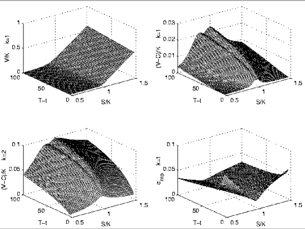
Figure 2: Option price and equivalent implied volatility in the risk-neutral approach to the stochastic volatility model

In Fig.2 we plot the option value surface for $V\left(S_{t},\sigma_{t},t\right)$ in the range $T-t\in[5,100]$ and $S/K\in[0.5,1.5]$ as well as the difference $\left(V\left(S_{t},\sigma_{t},t\right)-C\left(S_{t},\sigma_{t},t\right)\right)/K$ for $k=1$ and $k=2$. The other parameters are fixed at $\sigma=0.01,r=0.001,\delta=1,H=0.8$. The lower right panel shows the implied volatility surface corresponding to $V\left(S_{t},\sigma_{t},t\right)$ for $k=1$. Notice that computationally it is perhaps more convenient to use Eq.(39) (and an optimized Black-Scholes routine) than the more elegant Eq.(40).

4 An option pricing equation

Whenever the actual drift of a financial time series can be replaced by the risk-free rate we are in a risk-neutral situation. However, in stochastic volatility models this may not be a good assumption. In particular, an accurate option pricing formula should take into account the market price of volatility risk. Here we derive an option pricing equation which does not assume risk-neutrality.

Because volatility is not a tradable security, a pure arbitrage argument cannot determine completely the fair price of an option. On the other hand, because of the fractional nature of the volatility process, volatility follows a stochastic process different from the one of the underlying security. Therefore, we cannot apply the reasoning [33] that leads to uniform coefficients of the form $\left(\mu_{i}-\lambda_{i}\sigma_{i}\right)$ in the first derivative terms of the option pricing equation. Hence, a first principles derivation, with clearly specified assumptions is required.

As in Black-Scholes, we form a portfolio

$$\Pi\left(t\right)=V\left(S,\sigma,t\right)-\Delta\left(S,\sigma,t\right)S_{t}$$ (42)

From (11) and (18) and choosing $\Delta\left(S,\sigma,t\right)=\frac{\partial V}{\partial S}$ we obtain

$$d\Pi\left(t\right) = \left\{\frac{\partial V}{\partial t}+\frac{1}{2}\frac{\partial^{2}V}{\partial S^{2}}\sigma^{2}S^{2}\right\}dt+\sigma\frac{\partial V}{\partial\sigma}\frac{k}{\delta}\left(dB_{H}\left(t\right)-dB_{H}\left(t-\delta\right)\right)$$

$$+\left(\sigma^{2}\frac{\partial^{2}V}{\partial\sigma^{2}}+\sigma\frac{\partial V}{\partial\sigma}\right)H\frac{k^{2}}{\delta^{2}}\delta^{2H-1}dt$$

Consistent with our stochastic volatility model (9), we have assumed the volatility to be uncorrelated with $S$ and Eq.(4) follows from the application of the fractional Itô formula [21] [28]. Namely, if $X_{t}=\left(X_{t}^{(1)},X_{t}^{(2)},\cdots,X_{t}^{(n)}\right)$ with $dX_{t}^{(i)}=c_{i}\left(t,\omega\right)dB_{H}^{(i)}\left(t\right)$ , then

$$df\left(t,X_{t}\right)=\frac{\partial f}{\partial t}dt+\sum_{i}\frac{\partial f}{\partial X^{\left(i\right)}}dX_{t}^{(i)}+\sum_{i}\frac{\partial^{2}f}{\partial X^{\left(i\right)2}}c_{i}\left(t,\omega\right)D_{i,t}^{\phi}\left(X_{t}\right)$$ (44)

$D_{i,t}^{\phi}\left(X_{t}\right)$ being the $\phi-$Malliavin derivative corresponding to the $X_{t}^{(i)}-$process, defined by

$$D_{i,f}^{\phi}X_{t}\left(\omega_{i}\right) = \lim_{\varepsilon\rightarrow 0}\frac{1}{\varepsilon}\left\{X\left(\omega_{i}+\varepsilon\int_{0}^{\bullet}ds\int_{0}^{\infty}\phi\left(s,u\right)f\left(u\right)du\right)-X\left(\omega_{i}\right)\right\}$$

$$= \int_{0}^{\infty}D_{i,u}^{\phi}\left(X_{t}\right)f\left(u\right)du$$

$\phi\left(s,u\right)$ being the kernel

$$\phi\left(s,u\right)=H_{i}\left(2H_{i}-1\right)\left|s-u\right|^{2H_{i}-2}$$ (46)

In (4) we are still left with the stochastic term $\sigma\frac{\partial V}{\partial\sigma}\frac{k}{\delta}\left(dB_{H}\left(t\right)-dB_{H}\left(t-\delta\right)\right)$ and, because volatility is not a tradable security this term cannot be eliminated by a portfolio choice. Instead we may assume as reasonable to equate the deterministic term in $d\Pi\left(t\right)$ to

$$\left(r\Pi\left(t\right)+\nu\frac{k}{\delta}\sigma\frac{\partial V}{\partial\sigma}\right)dt$$ (47)

where $r$ is the risk-free return and, with $\nu>0$, the second term is a measure of the market price of volatility risk (bigger risk, bigger return). We end up with

$$\frac{\partial V}{\partial t}+rS\frac{\partial V}{\partial S}+\frac{\sigma^{2}S^{2}}{2}\frac{\partial^{2}V}{\partial S^{2}}+\frac{k}{\delta}\left(kH\delta^{2H-2}-\nu\right)\sigma\frac{\partial V}{\partial\sigma}+Hk^{2}\delta^{2H-3}\sigma^{2}\frac{\partial^{2}V}{\partial\sigma^{2}}=rV$$ (48)

as the general form of the option pricing equation consistent with the stochastic volatility model in (9).

We now obtain an integral representation for the solution of this equation. With the change of variable

$$x=\log\frac{S}{K}$$ (49)

and passing to the two-dimensional Fourier transform

$$V\left(t,x,\sigma\right)=\int\int d\phi d\rho F\left(\phi,\rho,\sigma\right)e^{i\left(\phi t+\rho x\right)}$$ (50)

we obtain

$$Hk^{2}\delta^{2H-3}\sigma^{2}\frac{\partial^{2}F}{\partial\sigma^{2}}+\frac{k}{\delta}\left(kH\delta^{2H-2}-\nu\right)\sigma\frac{\partial F}{\partial\sigma}+\left(i\left(\phi+\rho r-\frac{\sigma^{2}\rho}{2}\right)-\frac{\sigma^{2}\rho^{2}}{2}-r\right)F=0$$ (51)

Now, defining new constants

$$\begin{array}[]{lll}\chi\left(\rho\right)&=&\frac{\nu}{2Hk\delta^{2H-2}}\\ \xi^{2}\left(\rho,\phi\right)&=&\chi^{2}\left(\rho\right)-\frac{r-i\left(\phi+\rho r\right)}{Hk^{2}\delta^{2H-3}}\\ \zeta^{2}\left(\rho\right)&=&-\frac{i\rho+\rho^{2}}{2Hk^{2}\delta^{2H-3}}\end{array}$$ (52)

and making the replacement

$$F\left(\sigma\right)=\sigma^{\chi}Z_{\xi}\left(\zeta\sigma\right)$$ (53)

Eq.(51) reduces to a standard Bessel equation. Therefore the solution of (48) is

$$V\left(t,x,\sigma\right)=\int\int d\rho d\phi e^{i\left(\phi t+\rho x\right)}\sigma^{\chi\left(\rho\right)}Z_{\xi(\rho,\phi)}\left(\zeta\left(\rho\right)\sigma\right)$$ (54)

$Z_{\xi}\left(\zeta\sigma\right)$ being a Bessel function. The Bessel function will be a linear combination

$$Z_{\xi}\left(\zeta\sigma\right)=c_{1}J_{\xi}\left(\zeta\sigma\right)+c_{2}N_{\xi}\left(\zeta\sigma\right)$$

of a Bessel function of first kind and a Neumann function, with coefficients $c_{1}$ and $c_{2}$ to be fixed by the boundary conditions, which for call options is

$$V\left(T,x,\sigma\right)=\max\left(x,0\right)$$

Eq.(54) is an exact solution of the option pricing equation. How useful it might be will depend on the development of adequate computational algorithms for its numerical evaluation.

References

- [1] F. Black and M. Scholes; The pricing of options and coorporate liabilities, J. of Political Economy 81 (1973) 637-654.
- [2] R. C. Merton; Theory of rational option pricing, Bell J. Econ. Manag. Sci. 4 (1973) 141-183.
- [3] R. C. Merton; Option pricing when underlying stock returns are discontinuous, J. of Financial Economics 3 (1976) 125-144.
- [4] J. C. Cox and S. A. Ross; The valuation of options for alternative stochastic processes, J. of Financial Economics 3(1976) 145-166.
- [5] J. C. Cox, S. A. Ross and M. Rubinstein; Option pricing: A simplified approach, J. of Financial Economics 7 (1979) 229–263.
- [6] M. Rubinstein; Displaced diffusion option pricing, J. of Finance 38 (1983) 213-217.
- [7] J. C. Hull and A. White; The pricing of options on assets with stochastic volatility, J. of Finance 42 (1987) 281-300.
- [8] S. L. Heston; A closed form solution for options with stochastic volatility with applications to bond and currency options, The Review of Financial Studies 6 (1993) 327-343.
- [9] J.-P. Bouchaud and M. Potters; Theory of Financial Risk: From data analysis to risk management, Cambridge University Press 2000.
- [10] G. Bakshi, C. Cao and Z. Chen; Empirical performance of alternative option pricing models, J. of Finance 52 (1997) 2003-2049.
- [11] R. Tompkins; Stock index futures markets. Stochastic volatility models and smiles, The Journal of Futures Markets 21 (2001) 43-78.
- [12] S. Alizadeh, M. W. Brandt and F. X. Diebold; Range-based estimation of stochastic volatility models, J. of Finance LVII (2002) 1047-1091.
- [13] Zhuanxin Ding and C. W. J. Granger; Modeling volatility persistence of speculative returns. A new approach, J. Econometrics 73 (1996) 185-215.
- [14] F. J. Breidt, N. Crato and P. Lima; The detection and estimation of long memory in stochastic volatility models, J. of Econometrics 83 (1998) 325-348.
- [15] J. Vilasuso; Forecasting exchange rate volatility, Economics Letters 76 (2002) 59-64.
- [16] P. Embrechts and M. Maejima; Selfsimilar processes, Princeton Univ. Press, Princeton NJ 2002.
- [17] B. B. Mandelbrot and J. W. Van Ness; Fractional Brownian motions, fractional noises and applications, SIAM Rev. 10 (1968) 422-437.
- [18] B. B. Mandelbrot; Fractals and Scaling in Finance: Discontinuity, Concentration, Risk, Springer, New York 1997.
- [19] L. C. G. Rogers; Arbitrage with fractional Brownian motion, Math. Finance 7 (1997) 95-105.
- [20] L. Decreusefond and A. S. Üstünel; Stochastic analysis of the fractional Brownian motion, Potential Analysis 10 (1998) 177-214.
- [21] T. E. Duncan, Y. Hu and B. Pasik-Duncan; Stochastic calculus for fractional Brownian motion. I. Theory, SIAM J. Control Optim. 38 (2000) 582-612.
- [22] E. Alòs and D. Nualart; Stochastic integration with respect to the fractional Brownian motion, Stochastics and Stochastics Reports 75 (2003) 129-152.
- [23] Y. Hu; Heat equation with fractional white noise potentials, Applied Math. and Optimization 43 (2001) 221-243.
- [24] B. Øksendal and T. Zhang; Multiparameter fractional Brownian motion and quasi-linear stochastic differential equations, Stochastics and Stochastics Reports 71 (2001) 141-163.
- [25] E. Alòs, O. Mazet and D. Nualart; Stochastic calculus with respect to Gaussian processes, Ann. Probability 29 (2001) 766-801.
- [26] A. N. Shiryaev; On arbitrage and replication for fractal models, Research Report no. 2 MaPhySto, University of Aarhus 1998.
- [27] Y. Hu and B. Øksendal; Fractional white noise calculus and applications to finance, University of Oslo preprint 10/1999.
- [28] F. Biagini and B. Øksendal; Minimal variance hedging for fractional Brownian motion, University of Oslo preprint, February 2002.
- [29] E. M. Stein and J. C. Stern; Stock price distributions with stochastic volatility: An analytic approach, The Review of Financial Studies 4 (1991) 727-752.
- [30] B. LeBaron; Stochastic volatility as a simple generator of financial power laws and long memory, Quantitative Finance 2 (2001) 621-631.
- [31] R. Vilela Mendes, R. Lima and T. Araújo; A process-reconstruction analysis of market fluctuations, Int. J. of Theoretical and Applied Finance 5 (2002) 797-821.
- [32] C.-K. Peng, S. Havlin, H. E. Stanley and A. L. Goldberger; Quantification of scaling exponents and crossover phenomena in nonstationary heartbeat time series, Chaos 5 (1995) 82- 87.
- [33] Y.-D. Lyuu; Financial Engineering and Computation, Chapter 15, Cambridge Univ. Press, Cambrige UK 2002.