Magnetic-moment oscillations in a quantum Hall ring

Abstract

We predict non-mesoscopic oscillations in the orbital magnetic moment of a thin semiconductor ring in the quantum Hall effect regime. These oscillations, which occur as a function of magnetic field because of a competition between paramagnetic and diamagnetic currents in the ring, are a direct probe of the equilibrium current distribution in the nonuniform quantum Hall fluid. The amplitude of the oscillating moment in a thin ring with major radius $R$ and minor radius (half width) $a$ is approximately $aRe\omega_{\rm c}/c$, where $\omega_{\rm c}$ is the cyclotron frequency.

I introduction

There has been considerable interest in the orbital magnetic response of mesoscopic normal-metal rings to an applied magnetic field. The principal focus has been on the microscopic origin of the equilibrium persistent current $I$, which leads to a measurable magnetic moment $\pi R^{2}I/c$ in a thin ring of radius $R$. The persistent current $I$ is mesoscopic in originImry and vanishes in the macroscopic limit in accordance with Bloch’s theorem.Vignale However, because the current in a ring is actually distributed, the orbital magnetic moment

$$\mu\equiv{\pi\over c}\int\limits_{0}^{\infty}dr\ r^{2}j(r),$$ (1)

may be finite even if $I=\int_{0}^{\infty}dr\ j(r)$ vanishes. Here $j(r)$ is the azimuthal component of the equilibrium current density, and a two-dimensional electron system is assumed.

This multipole-moment effect is negligible in metal rings at laboratory magnetic field strengths or in semiconductor rings in weak fields, because $j(r)$ is itself small under these conditions. However, the equilibrium current density in the quantum Hall regime generally consists of strips or channels of distributed current, which alternate in sign, and which have universal (confining potential independent) integrated strengths of the order of $e\omega_{\rm c}$ Geller and Vignale ; Geller and Vignale CDFT . Therefore, although $I$ vanishes for a macroscopic ring in the quantum Hall regime, $\mu$ may be quite large. Furthermore, we shall show that because of a competition between paramagnetic and diamagnetic currents in the ring, the orbital magnetic moment oscillates with applied magnetic field. These oscillations, which are generally distinct from the de Haas–van Alphen or any mesoscopic oscillations, and which may be used to probe the equilibrium current distribution in the confined quantum Hall fluid, are the subject of this paper.

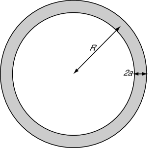
Figure 1: Two-dimensional electron gas in ring geometry.

There is an extensive literature on finite-size orbital magnetic effects in conductors,Denton ; Robnik ; Ruitenbeek ; Zhu and Wang and Sivan and Imry Sivan and Imry have discussed the de Haas–van Alphen oscillations in small (simply connected) quantum dots. The limit of a two-dimensional electron gas in a strong perpendicular magnetic field and a parabolic confining potential has been solved exactly by Harrison.Harrison However, we are not aware of any previous work on the problem considered here.

In the next section, we discuss the equilibrium current distribution in a ring in the quantum Hall effect regime, and we present results of a self-consistent Hartree calculation of the oscillating magnetic moment. In Section III, we show that in a particular limit, the magnetic-moment oscillations become that of the de Haas–van Alphen effect for a two-dimensional electron gas in the area defined by the bulk of the ring. Section IV contains a discussion of our results.

II hartree theory of the magnetic-moment oscillations

We shall assume that a two-dimensional electron gas is confined to a semiconductor ring of major radius $R$ and minor radius (half width) $a$ by a fixed positive background charge density of magnitude $n_{0}$. The inner radius of the two-dimensional ring is $R-a$ and the outer radius is $R+a$, as illustrated in Fig. 1. A uniform magnetic field of strength $B$ is oriented perpendicular to the two-dimensional electron gas in the $z$ direction.

The origin of the magnetic-moment oscillations is best understood within a self-consistent Hartree approximation. The effects of exchange and correlation are discussed at the end of this paper.

The theory of the equilibrium current distribution in the disorder-free, slowly confined quantum Hall fluid, has been developed in Refs. Geller and Vignale, and Geller and Vignale CDFT, . In the ring geometry considered here, the current flows in the azimuthal direction. The azimuthal component of the current density, a function of the radial coordinate $r$ only, may be written (ignoring exchange and correlation effects) as

$$j(r)=j_{\rm edge}(r)+j_{\rm bulk}(r),$$ (2)

where

$$j_{\rm edge}={e\hbar\over m^{*}}\sum_{i=0}^{\infty}\left(i+{\textstyle{1\over 2}}\right)\,{\partial n_{i}\over\partial r},$$ (3)

and

$$j_{\rm bulk}={en\over m^{*}\omega_{\rm c}}\,{\partial V\over\partial r}.$$ (4)

Here $m^{*}$ is the electron effective mass ($m^{*}/m\approx 0.067$ for GaAs), $e$ is the magnitude of the electron charge, and $\omega_{\rm c}\equiv eB/m^{*}c$ is the cyclotron frequency. In Eq. (3) $n_{i}(r)$ denotes the contribution to the equilibrium number density

$$n(r)=\sum_{i=0}^{\infty}n_{i}(r)$$ (5)

from the $i$-th Landau level, namely

$$n_{i}(r)\equiv{1\over 2\pi\ell^{2}}\sum_{\sigma}n_{\rm F}\left[\hbar\omega_{\rm c}\left(i+{\textstyle{1\over 2}}+{\textstyle{1\over 2}}\gamma\sigma\right)+V(r)\right].$$ (6)

Here $n_{\rm F}(\epsilon)=[\exp(\epsilon-\mu)/k_{\rm B}T+1]^{-1}$ is the Fermi distribution function,

$$\gamma\equiv{g\mu_{\rm B}B\over\hbar\omega_{\rm c}}={gm^{*}\over 2m_{\rm e}}$$ (7)

is the dimensionless spin splitting (with $g$ the magnitude of the effective Landé $g$-factor of the host semiconductor and $\mu_{\rm B}$ the Bohr magneton), $\ell\equiv\sqrt{\hbar c/eB}$ is the magnetic length, and the summation in Eq. (6) is over spin components $\sigma=\pm 1$. Instead of using the bare $g$-factor, which is about 0.44 in GaAs, we have used the experimentally measured exchange-enhanced value, which is aboutg7.3 $g\approx 7.3$ (see also Ref. g5.2, where a slightly smaller $g$-factor is observed). An important technical point in our computation is that the $g$-factor is the same for all Landau levels. This has been confirmed in an experimentg5.2 showing that the exchange-enhanced $g$-factor is independent of the magnetic field despite the intuitive expectation that it should have a $B^{-1/2}$ dependence (see Fig. 4 in Ref. g5.2, ). The confining potential $V(r)$ in Eq. (6) consists of an external potential, produced by the fixed positive background charge together with the self-consistent Hartree potential from the electron gas.confinement footnote The expressions above are valid provided $\ell V^{\prime}\ll\hbar\omega_{\rm c}$ and $k_{\rm B}T\ll\hbar\omega_{\rm c}$.

Assuming cylindrical symmetry, and a positive background charge given by $n_{\rm b}(r),$ the Hartree potential energy in the ring is

$$V(r)={4e^{2}\over\kappa}\int\limits_{0}^{\infty}\!dr^{\prime}\,{r^{\prime}\over r+r^{\prime}}\,K\left({4rr^{\prime}\over(r+r^{\prime})^{2}}\right)\bigg{[}n(r^{\prime})-n_{\rm b}(r^{\prime})\bigg{]},$$ (8)

where

$$K(m)\equiv\int\limits_{0}^{\pi/2}\frac{d\theta}{\sqrt{1-m\sin^{2}\theta}}$$ (9)

is the complete elliptic integral of the first kind,abramowitz-stegun (see Appendix A for more details) and $\kappa$ is the dielectric constant.

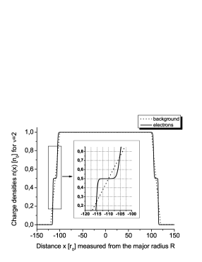
Figure 2: The electron density for $\nu=2$ (solid line) plotted together with the background charge density (dotted line) in units of $n_{0}=(2\pi r_{0}^{2})^{-1}$ for a two-dimensional ring of major radius $R=40a$ at temperature $T=0.005\ e^{2}/\kappa r_{0}k_{\rm B}$. The inset shows in more detail the inner-edge region where the $\nu=1$ incompressible strip is formed.

In Figs. 2 and 3 we present results of a self-consistent Hartree calculation of the low-temperature density and current distributions in the ring, as a function of $x\equiv r-R$ (the radial coordinate measured from the major radius of the ring). The dashed line in Fig. 2 shows the assumed positive background charge density of magnitude $n_{0}$ and width $2a$, where $a=100r_{0}$. Here $r_{0}$ is the average interparticle spacing in the bulk of the ring, defined by $n_{0}=(2\pi r_{0}^{2})^{-1}$. The background charge drops linearly to zero over a distance of $20r_{0}$, leading to the trapezoid-shaped cross-sectional distribution shown. The corresponding low-temperature electron density for a two-dimensional ring of major radius $R=40a$ is shown in the solid curve of Fig. 2. The magnetic field strength has been chosen so that two Landau levels are filled ($\nu=2$, where $\nu\equiv 2\pi\ell^{2}n_{0}$) in the bulk of the ring. Wide incompressible strips are formed at filling factor $\nu=1$ at the inner and outer edges of the ring.

The azimuthal current density at this same magnetic field strength is shown in the solid curve of Fig. 3 in units of $j_{0}\equiv e\hbar/2\pi m^{*}r_{0}^{3}$.

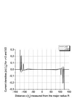
Figure 3: The current densities for $\nu=2$ (solid line) and $\nu=5/2$ (dotted line) in units of $j_{0}=e\hbar/2\pi m^{*}r_{0}^{3}$ for a two-dimensional ring of major radius $R=40a$ at temperature $T=0.005\ e^{2}/\kappa r_{0}k_{\rm B}$.

The qualitative features of the current distribution may be understood from Eqs. (3) and (4). At the inner edge of the ring, $x\approx-116r_{0}$, the density increases from zero to $n_{0}/2$. Because the compressibility in this edge region is large, the screening is nearly perfect and the self-consistent confining potential is approximately uniform. Therefore, the current density is dominated by the edge contribution (3). The current is positive because $n(r)$ is increasing with radius. At the boundary of the innermost edge region, $x\approx-114r_{0}$, the current has a node. In the $\nu=1$ incompressible region between $x\approx-114r_{0}$ and $-107r_{0}$, the density is uniform and the potential decreases by approximately $\hbar\omega_{\rm c}$. In this region the bulk contribution (4) is dominant, and the current is negative because $\partial V/\partial r$ is negative. At $x\approx-107r_{0}$ the incompressible region ends and there is another node in the current. Another edge region is then encountered as the density approaches its bulk value of $n_{0}$.

The current density at the outer edge of the ring follows similarly: There are two edge regions where the density decreases by $(2\pi\ell^{2})^{-1}$ and where the sign of the current is negative, separated by a $\nu=1$ incompressible bulk region where the current is positive. We note that the integrated current in each channel is universal, independent of the shape of the channel and the details of the confining potential.Geller and Vignale

It is tempting to regard the edge current (3) as being diamagnetic and the bulk current (4) as paramagnetic, but this is not correct. Figure 3 shows that the edge current—in the sense of our definition (3)—at the outer edge of the ring is in fact diamagnetic, but that near the inner edge of the ring it is paramagnetic instead.

At this point it is worth stressing the asymmetry between the odd-integer and even-integer filling factors $\nu$. It is well known that for the quantum Hall states with odd-integer $\nu$ the Fermi level resides in the Zeeman gap of size $\gamma\hbar\omega_{\rm c}$ within the uppermost Landau level, where $\gamma$ is defined in Eq. (7), while for the even-integer $\nu$ it lies in the cyclotron gap of size $\hbar\omega_{\rm c}$.

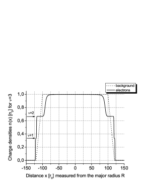
Figure 4: The electron density for $\nu=3$ (solid line) plotted together with the background charge density (dotted line) in units of $n_{0}=(2\pi r_{0}^{2})^{-1}$ for a two-dimensional ring of major radius $R=40a$ at temperature $T=0.005\ e^{2}/\kappa r_{0}k_{\rm B}$.

In our calculations, the spin-splitting is about 25% of the cyclotron energy. Because the width of the incompressible channel is proportional to the corresponding energy gap, the incompressible strips formed at odd-integer $\nu$ are notably narrower than the even-integer ones, as evident in Fig. 4. The horizontal arrows in Fig. 4 point to the positions of the incompressible strips corresponding to filling factors $\nu=1$ (at $n/n_{0}=1/3$) and $\nu=2$ (at $n/n_{0}=2/3$).

As the magnetic field is changed, the filling factor in the bulk of the ring changes. It is useful to define a dimensionless magnetic field strength

$$\beta\equiv{\hbar\omega_{\rm c}\over e^{2}/\kappa r_{0}},$$ (10)

where, as before, $\kappa$ is the dielectric constant of the semiconductor. The density of one filled Landau level is given by $(2\pi\ell^{2})^{-1}=r_{\rm s}\beta n_{0}$, where $r_{\rm s}\equiv r_{0}/a_{\rm B}$ is the dimensionless interparticle spacing and $a_{\rm B}\equiv\hbar^{2}\kappa/m^{*}e^{2}$ is the effective Bohr radius in the semiconductor. The density in Fig. 2 and current in the solid curve of Fig. 3 were calculated with the parameter values $r_{\rm s}=1$ and $\beta=1/2$.

The dotted curve of Fig. 3 shows the current distribution after the magnetic field has been reduced to a strength corresponding to $\beta=2/5$, so that $\nu=5/2$ in the bulk of the ring. In this case, there are three edge channels and two incompressible strips at the inner and outer edges of the ring. Note that the current distribution for $\beta=1/2$ and $\beta=2/5$ are almost everywhere opposite in sign (after an unimportant shift in $x$). This sign reversal, which clearly leads to oscillations in the orbital magnetic moment of the ring, occurs because of a combination of two factors: The competition between the edge current (3) and bulk current (4) leads to a pattern of strips or channels of current with alternating sign, and the electron-electron interaction expels most of the current from the bulk to the inner and outer edges of the ring.

The orbital magnetic moment of the ring is straightforward to compute from (1), and is plotted in the solid curve of Fig. 5 in units of

$$\mu_{0}\equiv 4\pi Ran_{0}\mu_{\rm B}^{*},$$ (11)

where $\mu_{\rm B}^{*}\equiv e\hbar/2m^{*}c$ is the effective Bohr magneton. The magnetic moment is plotted as a function of $\nu$, the filling factor in the bulk of the ring, and $r_{\rm s}=1$ as before. Note that the asymmetry between the odd-integer and even-integer $\nu$ discussed above leads to a partial suppression of the magnetization oscillation at odd-integer $\nu$. The dashed line of Fig. 5 shows the magnetic moment in the limit $R\gg a\gg\ell$ and $T=0$, which is calculated analytically in the next section. The deviation of the solid curve from the dashed one is a consequence of both finite-size effects and finite temperature. The solid curve on Fig. 5 is essentially the same as that in Fig. 2 of Ref. magnetization-exp, . The magnetic field distance between two adjacent minima of the magnetization in Fig. 2 in Ref. magnetization-exp, corresponds to a distance in $\nu$ approximately equal to 2 which is in very good agreement with Fig. 5 bellow.

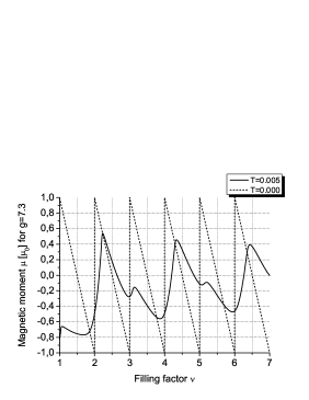
Figure 5: The magnetic moment as a function of the filling factor in units of $\mu_{0}$ for a two-dimensional ring of major radius $R=40a$ for temperature $T=0.005\ e^{2}/\kappa r_{0}k_{\rm B}$. The dashed line shows the oscillating magnetic moment of the noninteracting electron gas at $T=0$.

In addition to the plot of the magnetic-moment oscillations as a function of the filling factor $\nu$ given in Fig. 5, it is interesting to plot the magnetic moment as a function of the magnetic field. This is given in Fig. 6 for a system with $n_{0}=4.9\times 10^{15}m^{-2}\!$, corresponding to sample T412 of Ref. magnetization-exp, (after illumination), where we find excellent agreement with that experiment (see Fig. 3 of Ref. magnetization-exp, ).

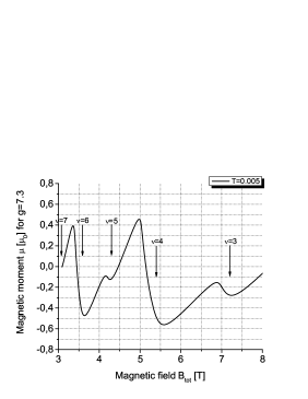
Figure 6: The magnetic moment (at temperature $T=0.005\ e^{2}/\kappa r_{0}k_{\rm B}$) as a function of the total magnetic field $B_{\rm tot}$ computed for the sample T412 of Ref. magnetization-exp, (after illumination) in units of $\mu_{0}$ for a two-dimensional ring of major radius $R=40a$. The arrows show the magnetic fields at which the corresponding filling factors appear.

III moment oscillations in the de haas–van alphen limit

In this section we calculate the orbital magnetic moment for the special case of $R\gg a\gg\ell$, a limit where an exact analytic solution is possible. Recall that $2a$ is the width of the electron gas in a ring of radius $R$, and $\ell$ is the magnetic length. We shall show that in this limit the magnetic-moment oscillations become that of the de Haas–van Alphen effect for a two-dimensional electron gas in the area defined by the bulk of the ring.

In terms of $x\equiv r-R$, the magnetic moment (1) may be written as

$$\mu={\pi\over c}\int\limits_{-\infty}^{\infty}dx\ (R+x)^{2}\ j(x),$$ (12)

where the fact that the current density vanishes outside the ring has been used to extend the limits of integration. Because $j(x)$ is an odd function of $x$ in a macroscopic ring in the $R\gg a$ limit [see Eq. (23) in Appendix A], we have

$$\mu={4\pi R\over c}\int\limits_{0}^{\infty}dx\ x\ j(x).$$ (13)

This expression shows that $\mu$ is proportional to the first moment of the current distribution shown in Fig. 3, which itself oscillates as a function of magnetic field.

Because the current density is concentrated at the inner and outer edges of the ring on a length scale much smaller than $a$,

$$\int\limits_{0}^{\infty}dx\ x\ j(x)\approx a\!\int\limits_{0}^{\infty}dx\ j(x).$$ (14)

Finally, the relation ${\bf j}({\bf r})=c\nabla\times{\bf M}({\bf r})$ between current and local magnetization shows that

$$\int\limits_{0}^{\infty}dx\ j(x)=c\ \!M(\nu),$$ (15)

where $M(\nu)$ is the $z$ component of the equilibrium orbital magnetization of a uniform two-dimensional electron gas with filling factor $\nu$.

Therefore, in the de Haas–van Alphen limit,

$$\mu=4\pi RaM(\nu).$$ (16)

The expression (16) shows that the magnetic moment in the $R\gg a\gg\ell$ limit is equal to that of a uniform electron gas of filling factor $\nu$ and area $4\pi Ra$, the area of the ring of width $2a$ and radius $R$. The magnetic moment in this limit, which may also be written as

$$\mu=\mu_{0}\ {M(\nu)\over\mu_{\rm B}^{*}n_{0}},$$ (17)

is shown at zero temperature in the dashed curve of Fig. 5.

IV discussion

In this paper, we have shown that the equilibrium current density in a confined quantum Hall fluid, which generally consists of a series of strips or channels of distributed current with alternating signs, leads to a magnetic moment in a non-mesoscopic ring that oscillates as a function of magnetic field. In a certain limit, namely $R\gg a\gg\ell$, the oscillations may be regarded as de Haas–van Alphen oscillations of the Hall fluid in the bulk of the ring, even though the current density in this limit is actually concentrated at the inner and outer edges.

The most natural interpretation of the magnetic-moment oscillations reported here is one in terms of the multipole moments of the equilibrium current distribution. The magnitude of the net current flowing at the edge of $\nu$ filled Landau levels is of the order of $\nu e\omega_{\rm c}$. This current contributes approximately $R^{2}\nu e\omega_{\rm c}/c$ to the orbital magnetic moment. However, the equilibrium currents flowing at the inner and outer edges of a macroscopic ring cancel, so the zeroth-order radial moment of the azimuthal current distribution, $\int_{-\infty}^{\infty}dx\ j(x)$, vanishes. However, the first radial moment, $\int_{-\infty}^{\infty}dx\ x\,j(x)$, does not vanish. The resulting magnetic moment is of the order of $\mu_{0}$, defined in (11), which may be equivalently rewritten as

$$\mu_{0}=\bigg{(}{a\over R}\bigg{)}\,R^{2}\nu e\omega_{\rm c}/c,$$ (18)

making evident its multipole-moment origin.

Finally, we note that the spin polarization contributes to the total the magnetic moment of the ring an amount

$$\mu_{\rm spin}=-{\textstyle{1\over 2}}g\mu_{\rm B}(N_{\uparrow}-N_{\downarrow}),$$ (19)

where $N_{\sigma}$ is the number of electrons with spin $\sigma$. The principal effect of exchange is to enhance the bare Zeeman spin splitting, which we have already accounted for phenomenologically by using $g$-factors deduced by experiments. The most important effect of correlation on the zero-temperature chemical potential and orbital magnetization of the uniform Hall fluid is to introduce additional discontinuities at certain fractional filling factors. This additional structure leads to incompressible strips and associated bulk currents at fractional filling factors in the nonuniform Hall fluid. It is clear from the analysis of Section III that in the $R\gg a\gg\ell$ limit, the orbital magnetic moment will reflect the actual orbital magnetization of the interacting electron gas. For other values of $R$ and $a$, we expect a more complex oscillatory response. Measurements of the magnetic moment of a semiconductor ring in the quantum Hall regime would provide useful information about the equilibrium current distribution in the nonuniform Hall fluid.

Appendix A The elliptic integral

The electrostatic potential produced by the electric charge distribution $\rho({\bf r^{\prime}})=e\,n(r^{\prime})\delta(z^{\prime})$ is explicitly independent of the polar angle $\phi$ and takes the form

$$V(r,z)=\frac{e^{2}}{\kappa}\int d^{3}r^{\prime}\frac{n(r^{\prime})\delta(z^{\prime})}{\sqrt{(\vec{r}-\vec{r}^{\prime})^{2}+(z-z^{\prime})^{2}}}$$

where $\vec{r}$ and $\vec{r}^{\prime}$ are the projections of the 3D vectors ${\bf r}$ and ${\bf r}^{\prime}$, respectively in the plane $z=0$. Let us choose the vector $\vec{r}$ to be in the direction of the $x$ axis so that $(\vec{r}-\vec{r}^{\prime})^{2}=r^{2}+{r^{\prime}}^{2}-2rr^{\prime}\cos\phi^{\prime}$ where $\phi^{\prime}$ is the polar angle of $\vec{r}^{\prime}$. After integrating over $z^{\prime}$ (and setting $z=0$) we get

$$V(r)=\frac{e^{2}}{\kappa}\int\limits_{0}^{\infty}r^{\prime}dr^{\prime}n(r^{\prime})\int\limits_{-\pi}^{\pi}\frac{d\phi^{\prime}}{\sqrt{r^{2}+{r^{\prime}}^{2}-2rr^{\prime}\cos\phi^{\prime}}}.$$ (20)

Noting that $\cos(-\phi^{\prime})=\cos(\phi^{\prime})$ and changing the integration variable $\phi^{\prime}=\pi-2\theta$ we can express the integral over $\phi^{\prime}$ in the above equation in terms of the complete elliptic integral (9), namely,

$$\frac{4}{r+r^{\prime}}K(m)\quad\mathrm{with}\quad m=\frac{4rr^{\prime}}{(r+r^{\prime})^{2}}.$$ (21)

Substituting Eq. (21) back into Eq. (20) one recovers the expression (8) that have been used in the self-consistent computation of the potential.

It is worth noting that in the de Haas-van Alphen limit in Sect. III, in which $R\gg a$, the electrostatic potential reproduces that of a thin infinite strip. The point is that $R-a\leq r,\,r^{\prime}\leq R+a$ and in this case $r\approx r^{\prime}\approx R$ so that $m\approx 1$ as seen from Eq. (21). However the elliptic integral (9) has a logarithmic asymptotics abramowitz-stegun for $m\to 1$

$$\lim_{m\to 1}\left[K(m)-\ln\left(\frac{4}{\sqrt{1-m}}\right)\right]=0,$$

where in our case $1-m=(r-r^{\prime})^{2}/4R^{2}$. Setting $r=R+x$ and $r^{\prime}=R+x^{\prime}$ we obtain

$$V_{\rm dHvA}(x)=-{2e^{2}\over\kappa}\int\limits_{-\infty}^{\infty}\!dx^{\prime}\,\ln\left|x-x^{\prime}\right|\bigg{[}n(x^{\prime})-n_{\rm b}(x^{\prime})\bigg{]},$$ (22)

where we have used $\int\!dx\ n(x)=\int\!dx\ n_{\rm b}(x)$. Equation (22) is exactly the potential of electrons in a 2D infinite strip with number density $n(x)$ and background charge density $-n_{\rm b}(x)$. It follows from Eqs. (3), (4), (6) and (22) that in the de Haas–van Alphen limit the potential and charge densities are even functions of $x$ while the current densities are odd

$$V(-x)=V(x),\quad n(-x)=n(x),\quad{\rm and}\quad j(-x)=-j(x)$$ (23)

which has been used in the derivation of Eq. (13). This symmetry is not present in a general two-dimensional electron ring.

References

- (1) Y. Imry, Introduction to Mesoscopic Physics (Oxford University Press, Oxford, 1997).
- (2) G. Vignale, Phys. Rev. B 51, 2612 (1995).
- (3) M. R. Geller and G. Vignale, Phys. Rev. B 50, 11714 (1994).
- (4) M. R. Geller and G. Vignale, Phys. Rev. B 52, 14137 (1995).
- (5) R. V. Denton, Z. Phys. 265, 119 (1973).
- (6) M. Robnik, J. Phys. A 19, 3619 (1986).
- (7) J. M. van Ruitenbeek, Z. Phys. D 19, 247 (1991).
- (8) J.-X. Zhu and Z. D. Wang, Phys. Lett. A 203, 144 (1995).
- (9) U. Sivan and Y. Imry, Phys. Rev. Lett. 61, 1001 (1988).
- (10) M. J. Harrison, Phys. Rev. B 45, 3815 (1992).
- (11) A. Usher, R. J. Nicholas, J. J. Harris and C. T. Foxon, Phys. Rev. B 41, 1129 (1990).
- (12) V. T. Dolgopolov, A. A. Shashkin, A. V. Aristov, D. Schmerek, W. Hansen, J. P. Kotthaus and M. Holland, Phys. Rev. Lett. 79, 729 (1997).
- (13) As is often the case with self-consistent Hartree and Hartree-Fock calculations in the quantum Hall effect regime, we find it necessary to include an additional hard-wall confining potential to V. Its precise form does not appreciably affect our results.
- (14) Handbook of Mathematical Functions, edited by M. Abramowitz and I. Stegun (Dover, New York, 1972).
- (15) A. Usher, M. Zhu, A. J. Matthews, A. Potts, M. Elliott, W. G. Herrenden-Harker, D. A. Ritchie and M. Y. Simmons, Physica E 22, 741 (2004).