Correlation between electrons and vortices in quantum dots

Abstract

Exact many-body wave functions for quantum dots containing up to four interacting electrons are computed and we investigated the distribution of the wave function nodes, also called vortices. For this purpose, we evaluate the reduced wave function by fixing the positions of all but one electron and determine the locations of its zeros. We find that the zeros are strongly correlated with respect to each other and with respect to the position of the electrons and formulate rules describing their distribution. No multiple zeros are found, i. e. vortices with vorticity larger than one. Our exact calculations are compared to results extracted from the recently proposed rotating electron molecule (REM) wave functions.

I Introduction

The discovery of the fractional quantum Hall effecttsui82 (FQHE) indicated the existence of a new state of matter corresponding to a novel type of strongly correlated quantum many-body state. Already the first steps towards the understanding of this effect involved the addition of extra zeros to the many-particle wave function in order to account for the electron-electron correlation. The Laughlin wave functionlaugh83l at filling factor $\nu=1/(2p+1)$ reads

$$\Psi=\prod_{j<k}(z_{j}-z_{k})^{2p+1}\exp\left[-\frac{1}{4}\sum_{l}|z_{l}|^{2}\right],$$ (1)

where units are used such that the magnetic length is set equal to unity. Here, $z=x-iy$ is a complex number expressing the two-dimensional coordinates of the electrons. If one fixes the coordinates of all electrons except one, the resulting wave function will have zeros of order $2p+1$ located at the positions of all fixed electrons. The wave function (1) embodies the strong correlation between the electrons as the wave function (and the probability to find an electron) in the vicinity of one of the fixed electrons vanishes more quickly than prescribed by the Pauli exclusion principle alone. We also note that in Laughlin’s wave function all the zeros are rigidly bound to the electrons and there are no free zeros. In this respect, the wave function (1) is rather special since a different distribution of zeros (e. g., around or between the fixed electrons) would also be able to serve the purpose of stronger correlation and reduced interaction energy.

In the subsequently formulated composite fermion (CF) theoryjain89 ; jain90 ; cf the strong correlations were dealt with in a different way, by introducing weakly interacting quasiparticles. Also here, the zeros of the many-body wave function played a central role. A zero in the wave function can also be interpreted as a vortex, i.e., when going around a zero its phase changes by $2\pi n$, and the winding number $n$ equals the order of the zero. The new quasiparticles of the CF theory were interpreted as electrons with an even number of vortices or magnetic field fluxes attached to them. When a particle moves around a closed loop it encircles the usual Aharonov-Bohm flux due to the external magnetic field which is partly cancelled by the vortices attached to the electrons. Therefore, the quasiparticles can be regarded as moving in an effective magnetic field which is much weaker than the applied magnetic field.

When constructing the CF wave function a Jastrow factor $(z_{k}-z_{l})^{2p}$ was introduced for each pair of electron coordinates, quite similarly to Laughlin’s wave function. Subsequently, the lowest-Landau-level (LLL) projection procedure, was introduced with the consequence that the vortices are no longer rigidly bound to the electrons. Thus, the relative distribution of zeros and electrons becomes less restrictive, and their correlations in this composite fermion liquid were investigated numerically in recent papers.graham03 ; pfann02 ; saar04

In the present paper, we investigate the electron-vortex correlations in a finite system by starting from exact many-body wave functions obtained by means of a direct numerical diagonalization. Our model system is a quantum dot containing a few (up to four) electrons. The numerical results are compared to those obtained from the analytically available rotating-electron-moleculeyann02 ; yann03 (REM) wave functions. This recently formulated theory appeared as a competitoryann03 (or at least an alternative) to the CF approach. It is derived from a more solid theoretical background, and introduces no a priori requirements on the positions of the zeros of the wave function.

The paper is organized as follows. The model, numerical procedure and the REM wave functions are described in Sec. II. The simple case of a two-electron quantum dot is described in Sec. III. Three- and four-electron dots are the subject of Secs. IV and V, respectively, and our conclusions are given in Sec. VI.

II Computational procedure

Let us consider a parabolic quantum dot with $N=2\,\ldots\,4$ electrons placed into a perpendicular magnetic field of strength $B$. We work with dimensionless oscillator units,maarten03 that is, lengths are measured in oscillator lengths $a_{0}=(\hbar/m^{*}\omega_{0})^{1/2}$ and energies in $\hbar\omega_{0}$ where $\omega_{0}$ is the confinement frequency. Then the relative strength of the inter-electron interaction is given by the dimensionless coupling constant $\lambda=a_{0}/a_{B}^{*}$ expressed as a ratio of the oscillator length to the effective Bohr radius $a_{B}^{*}=\varepsilon\hbar^{2}/e^{2}m^{*}$. Here, $\varepsilon$ is the dielectric constant of the medium and $m^{*}$ is the effective electron mass. The magnetic field strength is expressed as a ratio of the cyclotron and confinement frequencies $\gamma=\omega_{c}/\omega_{0}$. The resulting dimensionless Hamiltonian

$$\hat{H} = \frac{1}{2}\sum_{i=1}^{N}\left[-\nabla_{i}^{2}+\left(1+\frac{\gamma^{2}}{4}\right)r_{i}^{2}\right]+\frac{\gamma}{2}L$$ (2)

$$+ \sum_{{i,j=1}\atop{i>j}}^{N}\frac{\lambda}{|\mathbf{r}_{i}-\mathbf{r}_{j}|},$$

is solved by direct diagonalization in the subspaces of given angular momentum $L$, which is a good quantum number. The results regarding the dependence of the ground state angular momentum on the confinement and the magnetic field strength for the case of four electrons in the dot were analyzed in Ref. maarten03, . Throughout this paper we take $\lambda=2$ which is a typical value for experimental realized quantum dots.tar01 We found that higher values of $\lambda$ require longer calculations timesmikh4 and did not result in new physics.

In the present work we concentrate on the fully polarized ground states and investigate the information encoded in the corresponding ground state many-body wave function

$$\Psi(\mathbf{r}_{1},\ldots,\mathbf{r}_{N}),$$ (3)

or, to be more precise, on the reduced wave function, which depends only on the position of one electron while the coordinates of the remaining $N-1$ electrons are set to fixed values. Due to the Pauli principle, the reduced wave function has zeros at the positions of the fixed electrons. There are additional zeros which are not fixed at the electrons whose distribution will be the main object of interest in the present work. In order to locate the positions of the vortices we first locate the positions of the minima of the squared absolute value of the reduced wave function using a standard procedure of steepest descent from a randomly chosen initial point. Then, by performing a walk along a small circle around the located points and inspecting the change of the phase of the wave function we are able to distinguish actual zeros from other minima and determine their order, i. e. the winding number.

We complement the results obtained from the exact diagonalization (ED) by those given by the REM wave functions.yann02 ; yann03 These functions are available analytically and help to make some exact statements. These functions are constructed by placing Gaussians at the classical positions of electrons in strong magnetic fields and a subsequent restoration of symmetry. For a small number of electrons ($N\leq 5$), the electrons crystallize into a single ringbed94 and the resulting wave function of the angular momentum $L$ readsyann03

$$\Psi_{L} = \sum_{0\leq l_{1}<l_{2}<\ldots<l_{N}}^{l_{1}+\ldots l_{N}=L}\left(\prod_{j=1}^{N}l_{j}!\right)^{-1}$$ (4)

$$\times \left(\prod_{1\leq j<k\leq N}\sin\left[\frac{\pi}{N}(l_{j}-l_{k})\right]\right)$$

$$\times {\cal D}(l_{1},l_{2},\ldots,l_{N})\exp\left(-\sum_{j=1}^{N}z_{j}z_{j}^{*}/2\right).$$

Here, $z_{j}$ denote the complex electron coordinates measured in units $l_{c}\sqrt{2}$ with $l_{c}=\sqrt{\hbar c/eB}$ being the magnetic length, and ${\cal D}$ is the Slater determinant

$${\cal D}(l_{1},l_{2},\ldots,l_{N})=\mathrm{det}[z_{1}^{l_{1}},z_{2}^{l_{2}},\ldots,z_{N}^{l_{N}}].$$ (5)

The wave function describes spin-polarized states of angular momentum $L=L_{0}+Nm$ where $L_{0}=N(N-1)/2$ is the smallest possible angular momentum of $N$ spin-polarized electrons in the lowest Landau level, and $m$ is a non-negative integer.

Already from the general form of the REM wave function (4) several conclusions regarding the distribution of zeros of the reduced wave function can be drawn. First, as far as the positions of zeros are concerned, the exponential factor in Eq. (4) can be ignored, that is zeros can be found from the linear combination of the Slater determinants which expands into a homogeneous polynomialyann02 $P_{L}[z]$ of order $L$. Therefore, scaling the coordinates of all fixed electrons $z_{j}\to\alpha z_{j},j=1,\ldots,N-1$ results in scaling of the positions of zeros. Moreover, the polynomial $P_{L}[z]$ is translationally invariantyann02 , therefore rigid shifting of the positions of the fixed electrons by the same amount results in a rigid translation of the distribution of zeros in the $z_{N}$ plane. Due to the circular symmetry of the quantum dot, the distribution of wave function zeros is also invariant with respect to rotation of the system as a whole.

Regarded as a function of $z_{N}$ the order of the polynomial $P_{L}[z]$ is $q_{N}=L-(N-1)(N-2)/2$. This follows from the fact that in order for one electron to occupy the orbital with the largest possible angular momentum $l$, the remaining $N-1$ electrons must reside in the lowest possible momentum states $l=0,1,\ldots,N-2$. Thus, according to a fundamental theorem of algebra the total number of zeros is $L$ for two electrons, $L-1$ for three electrons, and $L-3$ for a four electron system.

The question of the number of zeros obtainable from exact diagonalization is more subtle. If the ED procedure includes only the single-electron states from the lowest Landau level, the resulting wave function is a polynomial times a Gaussian, i. e. has a similar structure to the REM wave function but the expansion coefficients are now determined numerically. Thus, in the case of the lowest-Landau-level approximation we expect to find the same number of vortices as predicted from the REM wave function. However, if higher Landau levels are included the ED wave function (with the exponential removed) involves Laguerre polynomials of the argument $|z_{j}|^{2}$ and thus becomes non-analytical. This fact prevents us from making any exact statements regarding the total number of zeros. However, in the high magnetic field limit the lowest Landau level approximation becomes rather accurate and inclusion of higher Landau levels modifies the calculated wave function only at large distances from the quantum dot center. Thus one may still expect to find the same number of zeros as predicted from the earlier argument.

On the other hand, the non-analyticity of the ED wave function makes it possible to observe besides vortices also anti-vortices, i. e. zeros around which the phase winds in the opposite direction.

III Two-electron quantum dot

Figure 1: The phase of the reduced wave function for two electrons. One electron is fixed at $\mathbf{r}=(1,0)$. The angular momentum of the state is $L=7$ and we find a seventh order zero located exactly at the fixed electron. Lengths are measured in units of $a_{0}$

For the sake of completeness, we begin with the simplest case of two electrons in a dot. We evaluate the reduced wave function in a ground state of angular momentum $L=7$ and plot its phase as a function of the coordinates in Fig. 1. One electron is fixed at $(x,y)=(1,0)a_{0}$. Different shades of gray correspond to different values of the phase between $-\pi$ and $\pi$. Zeros of the wave function are located at the points where the phase is not determined and the winding number indicates the order of the zero. We see that in the present case we have a single zero of seventh order located at the position of the fixed electron.

This result can be easily understood by recalling that in a parabolic confinement potential the center-of-mass (CM) motion and the relative motion can be separated. The CM motion is not affected by the electron-electron interaction. In the ground state the CM motion is in its lowest state and its wave function is just a Gaussian of the CM coordinate which does not lead to the appearance of any zeros. The wave function of the relative motion at small values of the relative coordinate $\mathbf{r}=\mathbf{r}_{1}-\mathbf{r}_{2}$ behaves as $\sim r^{m}\,e^{im\phi}$ where the relative angular momentum $m$ coincides with the total momentum $L$. Therefore, in the reduced two electron wave function one always finds just a single “giant” vortex of vorticity $L$.

Note that this situation is special to the parabolic confinement case, and deviations from perfect parabolicity leads to splitting of the multiple vortex to a system of several single vortices. This was found in the reduced wave function of two electrons in a confined trionme03 where the non-parabolicity of the potential felt by electrons was due to the presence of a nearby hole.

IV Three electrons in a dot

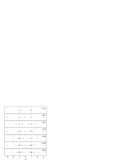
Figure 2: The location of the zeros of the reduced wave function in a three-electron quantum dot for different values of the angular momentum $L$, calculated with the ED method. Two electrons are fixed at $\mathbf{r}=(1,0)$ and $\mathbf{r}=(-1,0)$. The zeros located on the pinned electrons are indicated by crosses and the dots mark the free zeros. Note that all zeros fall on a single straight line. Lengths are measured in units of $a_{0}$.

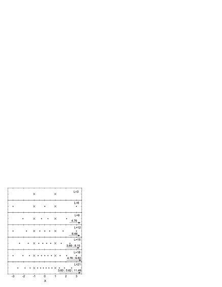
Figure 3: The same as in Fig. 2 but now for the REM wave function. The number of observed zeros is the same, however, their clustering around the fixed electrons is not seen. The arrows indicate vortices which are outside the plotted region. They are only indicated on the right side, but evidently are also present on the left side. Note that for the REM result lengths are originally measured in units of $l_{c}\sqrt{2}$, but can be perfectly rescaled to units of $a_{0}$ to match with the ED result.

The locations of the zeros calculated with the ED method for the $N=3$ case are shown in Fig. 2 for the spin-polarized ground states up to $L=21$. The angular momenta of these states are multiples of $3$ as predicted by the magic number theory.ruan1 The two fixed electrons are located at $(x,y)=(\pm 1,0)a_{o}$. We observe that all zeros appear on a straight line defined by the two pinned electrons (crosses in Fig. 2). This result persists also when the two pinned electrons are located off the $y=0$ axis, and the distances between the zeros are not visibly changed.

In the case of $L=3$ we find only two vortices located at the positions of the fixed electrons. Increasing the angular momentum to $L=6$ results in the addition of three vortices, one is placed between the fixed electrons and one on each side. The total number of observed vortices in this case is $L-1$ as predicted by the simple estimate. Proceeding to higher angular momenta, we see that at each step one more vortex is inserted between the fixed electrons. Whether or not each time one extra vortex is added on each outer side of the electrons is difficult to say. The reason is that at large distances from the origin (typically $r>4$), the accuracy of the wave function becomes insufficient due to the limited basis set used in the numerical calculation. Inaccuracies may result in “ghost” vortices. Therefore, the calculations were limited to $r\approx 3.5$ (beyond which the electron density becomes very small, i. e. typically $|\Psi|^{2}<10^{-6}$) and some vortices located outside this region may be overlooked. On the other hand, for the REM method, all vortices can be found, including those outside $r<4$, which are indicated with arrows in Fig. 3.

Addition of the new vortices between or on the outer side of the fixed electrons leads to a rearrangement of the vortices which were already present. The vortices are pushed towards each other and in particular towards the fixed electrons. This can be nicely seen for $L=9,12,15,18,21$ in Fig. 2 where the pinned electrons (indicated by the crosses) are approached by two vortices, and later by four.

With increasing $\gamma$ higher angular momentum states become the ground state. Keeping the angular momentum fixed and letting $\gamma$ change shows that the effect of the magnetic field on the positions of the vortices is surprisingly small. For example, for the $L=12$ state the position of the vortex around 0.75 ranged from 0.74 to 0.76 for $0<\gamma<15$. This implies that the position of the vortices is mainly determined by the value of the angular momentum. Since we are not interested in the exact position of the vortices but rather in their general behavior and their interactions, we will from now take $\gamma=2$.

In Fig. 3 we show the distribution of the zeros for the same angular momenta and the same fixed electron positions as in Fig. 2 but now obtained from the REM wave functions. We see that most of the qualitative features are well reproduced except for their positions in case of $L>6$. Note that between the fixed electrons the zeros are more uniformly distributed and the clustering around the electrons as seen for the ED method is absent.

As a matter of fact, for the case of three electrons the positions of zeros in the REM theory can be calculated exactly. Introducing the center-of-mass coordinate $\bar{z}=(z_{1}+z_{2}+z_{3})/3$ and two relative (Jacobijacak98 ) coordinates

$$z_{a} = \sqrt{\frac{2}{3}}\left[\frac{z_{1}+z_{2}}{2}-z_{3}\right],$$

$$z_{b} = \frac{z_{1}-z_{2}}{\sqrt{2}},$$ (6)

and dropping the exponential factors in Eq. (4) the polynomial part of the REM wave function can be writtenyann02 in a particularly simple form

$$P_{L}(z_{a},z_{b})=(z_{a}+iz_{b})^{L}-(z_{a}-iz_{b})^{L}.$$ (7)

Equating (7) to zero and taking the $L$-th order root we find

$$z_{a}+iz_{b}=(z_{a}-iz_{b})\exp(2\pi ik/L),\quad k=1,2,\ldots,L-1.$$ (8)

Note that there are $L-1$ roots as the meaningless root $k=0$ has to be omitted. Eq. (8) is readily solved with the result $z_{a}=z_{b}\,\textrm{cotan}(\pi k/L)$, and using the specific values $z_{1,2}=(\pm 1,0)$ we find the positions of the roots

$$z_{3}=\sqrt{3}\,\textrm{cotan}\left(\frac{\pi k}{L}\right),\quad k=1,2,\ldots,L-1.$$ (9)

Note that despite using the specific values for the coordinates of the fixed electrons this result is still general since employing the above discussed symmetry properties of the REM wave functions any randomly fixed two electron positions (for $N=3$) can be mapped on $(\pm 1,0)$.

The result given in Eq. (9) correctly predicts the appearance of all zeros on a single straight line and reveals a simple rule for their distribution. The angular momentum for which the REM function is valid must be a multiple of $3$, that is $L=3n$ with $n$ being an integer. Therefore, among the roots (9) there always are two (namely, $k=n$ and $k=2n$) whose positions $z_{3}=\pm 1$ coincide with the fixed electrons. Moreover, these two solutions, $k=n$ and $k=2n$, divide the interval $k=1,\ldots,L-1$ into three equal parts. Thus, we can confirm the rule which was already apparent in the ED results: each time when the angular momentum is increased by $3$, three new vortices enter the quantum dot, and one of them is placed between the fixed electrons while the other two on the outer sides (some of the latter zeros are indicated outside the plotted x-region in Fig. 3). This is in agreement with our ED results when we limit ourselves to the $|x|<3.5$ region. Our results are in variance with those of Saarikoski et al. [saar04, ] who found only the addition of a single vortex when $L$ increases to its subsequent allowed value.

Note that the analytic expression (9) obtained from the REM theory fails to predict the clustering of zeros around the fixed electrons. Namely, Eq. (9) suggests that the density of vortices is largest around $z_{3}=0$ and monotonically decreases to both sides. this is opposite to the ED result which clearly shows that the density of vortices tends to increase around the fixed electrons and is somewhat lower right in the middle between the two electrons. The REM approach is unable to reflect the subtle interaction between the electrons and the zeros but at larger distances from the pinned electrons it predicts the zeros at approximately the correct positions, as can be seen for $L=6,12,18$ around $x=3$.

V Four electrons

In the $N=4$ case the three pinned electrons can be placed in many different ways. We consider three main configurations: a half-square triangle (corresponding to the classical positions in a Wigner crystalbed94 ), an equilateral triangle and a line configuration.

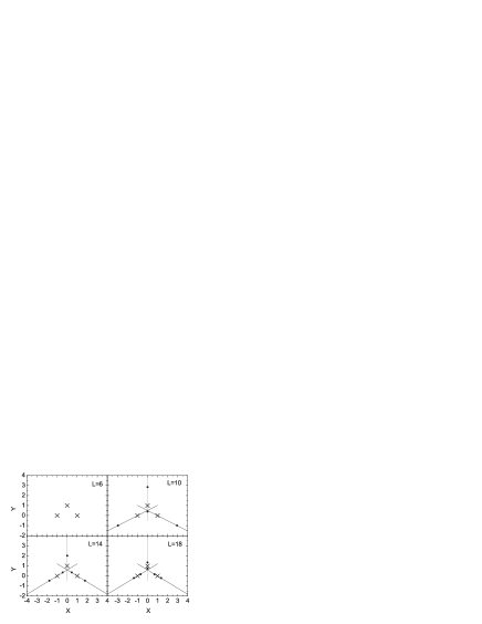
Figure 4: The location of the zeros of the reduced wave function for four electrons for different angular momenta $L$, calculated with the ED method. Three electrons are fixed at $\mathbf{r}=(\pm 1,0)$ and $\mathbf{r}=(0,1)$ forming a half-square configuration. Lengths are measured in units of $a_{0}$.

Fig. 4 shows the positions of zeros corresponding to the half-square triangle configuration, calculated with the ED method. The pinned electrons are located at $\mathbf{r}=(\pm 1,0)$ and $\mathbf{r}=(0,1)$, i.e. at the three corners of a square, and the considered angular momenta are $L=6,10,14,18$, i. e. the ones corresponding to the full spin polarization in the ground state. One immediately notices that the positions of the zeros of the wave function are arranged on rays (shown by the thin lines in Fig. 4. Again, it is possible to spot a simple rule analogous to the one obtained for the preceding three-electron case that explains the location of the zeros. At the lowest possible angular momentum $L=6$ there are three zeros whose positions coincide with the pinned electrons. Each time the ground state angular momentum is increased by four, four new zeros are added. One is placed inside the triangle defined by the three pinned electrons and the other three end up on the rays outside the triangle. In this case we looked at points up to $r\approx 4$ from the origin, thus some of the zeros are located outside this region, where $|\Psi|^{2}$ is negligible small. One notices again that the free zeros, seem to gather around the pinned electrons, which is clearly seen, e. g., for $L=18$. Note that the $L=18$ state corresponds to the $\nu=1/3$ Laughlin state following the formula $\nu=\frac{N(N-1)}{2L}$. In Fig. 4 one can actually see three vortices (one attached to the pinned electron and two free vortices) in the close neighborhood of the pinned electrons.

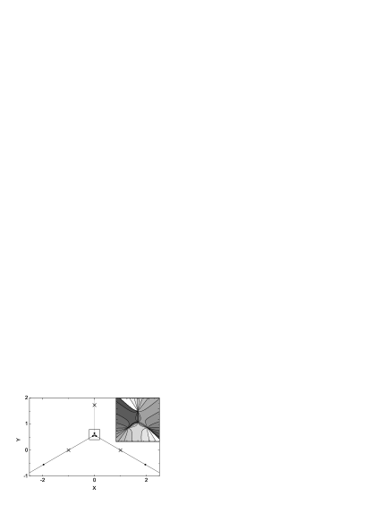
Figure 5: The location of the zeros of the reduced wave function for four electrons when $L=14$ for the equilateral triangle configuration, calculated with the ED method. Three electrons are fixed at $\mathbf{r}=(\pm 1,0)$ and $\mathbf{r}=(0,\sqrt{3})$. An anti-vortex appears around $\mathbf{r}=(0,0.5)$ indicated by the open dot. The inset shows a contourplot of the phase near the position (indicated by the square in the main figure) of the anti-vortex. Lengths are measured in units of $a_{0}$.

The number of zeros inside the triangle formed by the pinned electrons increases by one each time the angular momentum increases by four. So, for $L=14$ there are two zeros located inside the triangle, and it is interesting to see how their arrangement can agree with the external symmetry defined by the pinned electrons when the half-square triangle is transformed into an equilateral one. As can be seen from Fig. 5, instead of two zeros inside the triangle four zeros are formed. One of them is placed into the center and actually is an anti-vortex (see inset of Fig. 5 for a contourplot of the phase of the wave function), while the other three vortices are arranged on the vertices of an equilateral triangle, thus the symmetry adapts to the external symmetry and the total vorticity is preserved. Apparently this configuration is preferred over merging of two zeros into a single one with vorticity two (which would be sufficient to adapt to the symmetry). This phenomenon shows that the zeros do not like to sit on the same spot, and there is a certain repulsion between them, i. e. there is a clear tendency not to form vortices with winding number $n>1$. As a rule we may state that we can expect the formation of anti-vortices by this rule whenever the symmetry implied by the pinned electrons forces vortices to come close. This will be the case for $L=26$ in this system, but it will also be the case in systems with more electrons.

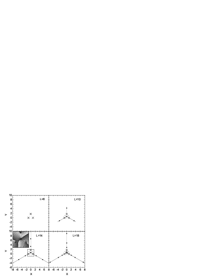
Figure 6: The location of the zeros of the reduced wave function for four electrons for different angular momenta $L$, calculated with the REM method. Three electrons are fixed at $\mathbf{r}=(\pm 1,0)$ and $\mathbf{r}=(0,\sqrt{3})$. The zeros located on the pinned electrons are indicated with a cross and the free zeros are indicated with a dot. Note that the zero in the middle for $L=14$ is in fact a giant vortex of vorticity 2 as is apparent from the inset which shows a contourplot of the central region.

This result is in contrast with the REM result which predicts that the two zeros inside the triangle join into one giant vortex, as can been seen from Fig. 6 for $L=14$. Apparently, the REM is not capable of describing the subtle interaction between the zeros due to its restriction to analytic wave functions. One also notes that again in REM there is no congregation of zeros around the pinned electrons in Fig. 6 and like for $N=3$ the vortices rather tend to accumulate in the center between the electrons.

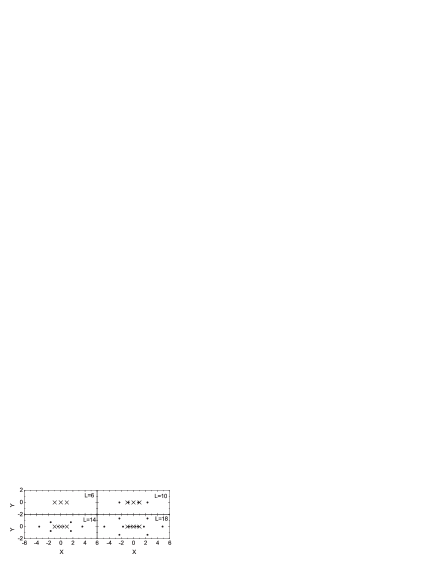
Figure 7: The location of the zeros of the reduced wave function for four electrons for different angular momenta $L$, calculated with the REM method. Three electrons are fixed at $\mathbf{r}=(\pm 1,0)$ and $\mathbf{r}=(0,0)$. The zeros located on the pinned electrons are indicated with a cross and the free zeros are indicated by a dot.

One may wonder how strong the exact location of the fixed electrons influences the positions of the vortices. Therefore, we consider the case of a line arrangement of the electrons. In Fig. 7 we show the location of the zeros for a line configuration calculated with the REM method. The three electrons are fixed at $\mathbf{r}=(\pm 1,0)$ and $\mathbf{r}=(0,0)$. Notice that for $L=14$ there are two vortices between the electrons in contrast to the previous cases shown in Figs. 4 and  6 where only one vortex is situated in the area between the electrons. The reason is that a single vortex would be located on top of the middle electron. The system tries to prevent to have higher-order zeros and resolves this issue by taking one of the vortices, which was previously (see Figs. 4 and  6) outside the inner electron region, and placing it between the electrons which results in a symmetric distribution of vortices. In contrast to the two electron case, there are zeros which appear next to the line defined by the three pinned electrons. When we look at the locations we can derive a simple rule that explains the addition of the vortices: every time one goes to the next magic angular momentum four zeros are added. The first time they are added on the $y=0$ line and are equally distributed in between the pinned electrons. In the next step they are added symmetrically above and below the $y=0$ line. These two rules alternate each time the angular momentum is increased by four.

Table 1: The polynomials $Q_{L}(z)$ for the case when three pinned electrons are situated on a single line.

$L$	$Q_{L}(z)$
6	$1$
10	$3z^{4}-18z^{2}+10$
14	$3z^{8}-52z^{6}+212z^{4}-448z^{2}+80$
18	$3z^{12}-102z^{10}+990z^{8}-6160z^{6}+14003z^{4}$
	$-7837z^{2}+291$

In the case of four electrons in the dot it is not possible to derive and solve a general compact expression for the polynomial describing the distribution of zeros in the REM wave function as it was done for the three-electron dot. For the present configuration featuring the arrangement of three pinned electrons into one line such polynomial has the form $z(z^{2}-1)Q_{L}(z)$ where the first two factors represent the zeros located on the fixed electrons, and the polynomial $Q_{L}(z)$ describes the distribution of the vortices. In Table 1, we give this polynomial for the considered values $L=6,10,14,18$. Note that thanks to the symmetry of the configuration only even $z$ powers appear in $Q_{l}(z)$.

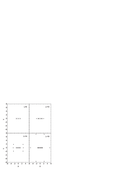
Figure 8: The same as in Fig. 7 but calculated with the ED method. Three electrons are fixed at $\mathbf{r}=(\pm 1,0)$ and $\mathbf{r}=(0,0)$. Lengths are measured in units of $a_{0}$

Next we compare the previous REM results with our exact calculation. Therefore, we show in Fig. 8 the same configuration as in Fig. 7 but now the results are obtained with the ED method. The location of the zeros is qualitative similar to those for the REM functions, but again we see that there is a much stronger clustering around the fixed electrons and the vortices above and below the $y=0$ line are much further away.

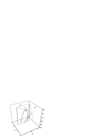
Figure 9: The position of the inner vortices as a result of the movement of the fixed electrons for $L=14$. Two electrons are fixed at $\mathbf{r}=(\pm 1,0)$ and the third one is fixed at $\mathbf{r}=(0,z)$. The projections of the vortex positions on the $x=0$ and $y=0$ planes are given by dashed lines for clarity. The triangle itself is indicated by dotted lines. The open dots indicate the region of existence of the anti-vortex. Only the three fixed electrons forming the triangle and the vortices inside the triangle are shown. Lengths are measured in units of $a_{0}$.

To summarize the dependence of the location of the vortices on the positions of the fixed electrons we show in Fig. 9 a 3D plot for $L=14$ in which we fix two electrons at $\mathbf{r}=(\pm 1,0)$ and move the third electron along the vertical axis from $\mathbf{r}=(0,0)$ to $\mathbf{r}=(0,2)$. Notice that we can clearly see: (1) how the vortices move with changing symmetry of the fixed electron distribution, (2) the appearance of an anti-vortex when the two inner vortices come close to each other and (3) how the anti-vortex exist over a certain range before merging with a vortex and being annihilated, and (4) how the position of the two vortices are rotated over $90^{\circ}$ with respect to the position of the electrons when one electron moves away from the two others, i. e. with increasing $z$. This rotation occurs through the intermediate creation of an anti-vortex.

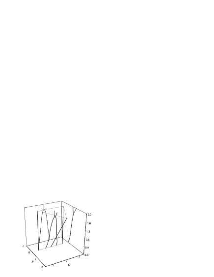
Figure 10: Same as in Fig. 9 but now calculated with the REM method. Notice that there is no anti-vortex present.

Similar results for the REM reduced wave function are shown in Fig. 10. One observes that also here the relative position of the vortices are rotated over $90^{\circ}$ but that in this case no anti-vortex is formed to make this happen, i. e. the two vortices join in one giant vortex of vorticity two and then they separate again into two distinct vortices.

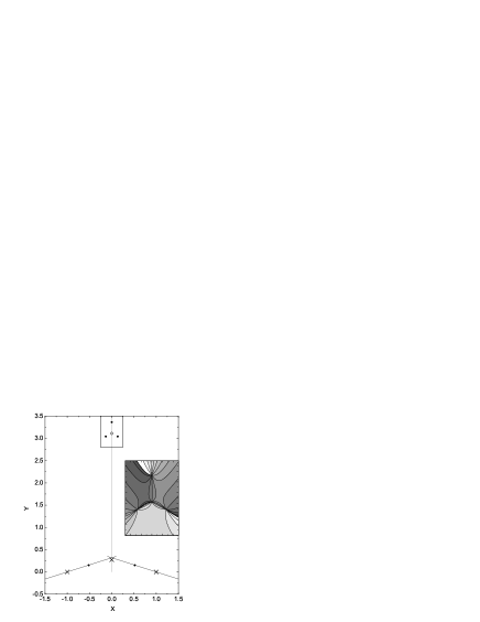
Figure 11: Vortex positions calculated with the ED method for $L=14$. Three electrons are fixed at $\mathbf{r}=(\pm 1,0)$ and $\mathbf{r}=(0,0.273)$. The zeros located on the pinned electrons are indicated with a cross and the free zeros are indicated by a dot. A anti-vortex (open dot) appears at $\mathbf{r}=(0,3)$. The inset shows the phase of the reduced wave function around the anti-vortex. Lengths are measured in units of $a_{0}$.

Another interesting thing to investigate is the evolution from a triangle configuration towards a line configuration. As Fig. 8 shows for $L=14$ two vortices are located above the $y=0$ line at $\mathbf{r}=(\pm 2.6,1.8)$ and two below at $\mathbf{r}=(\pm 2.6,-1.8)$. When we start moving the fixed electron at $\mathbf{r}=(0,0)$ upwards the two vortices located above the $y=0$ line will move closer to each other and finally a vortex-anti-vortex pair will be created as soon as they are close enough as shown in Fig. 11. Going further a vortex and an anti-vortex will meet and annihilate, changing the configuration to one with two vortices located on the $x=0$ line. The mechanism behind this is the same as shown in Fig. 9.

VI Conclusions

We investigated the distribution of zeros of the reduced many-body wave function in few-electron quantum dots. The results show that the arrangement of zeros can be described by a set of simple rules. The number of vortices increases with $\Delta l=N$ between two subsequent fully polarized magic angular momentum states. The vortices (or zeros) between the electrons are situated on rays pointing away from the electron cluster. There is clear evidence of repulsion between the zeros and their attraction to the pinned electrons leading to a strong correlation between the vortices and between the electrons and the individual vortices. Additional vortex-anti-vortex pairs can be formed for certain symmetries of the fixed electron distribution. Qualitatively, several of the results on the distribution of the zeros can be obtained from an analytically available rotating-electron-molecule wave functions. However, the REM theory is not able to describe the condensation of zeros around fixed electrons and the formation of an anti-vortex.

- (1) D. C. Tsui, H. L. Stormer, and A. C. Gossard, Phys. Rev. Lett. 48, 1559 (1982).
- (2) R. B. Laughlin, Phys. Rev. Lett. 50, 1395 (1983).
- (3) J. K. Jain, Phys. Rev. Lett. 63, 199 (1989).
- (4) J. K. Jain, Phys. Rev. B41, 7653 (1990); ibid. 42, 9193(E) (1990).
- (5) Composite Fermions: a unified view of the quantum Hall regime, editted by O. Heinonen (World Scientific, Singapore, 1998).
- (6) K. L. Graham, S. S. Mandal, and J. K. Jain, Phys. Rev. B67, 235302 (2003).
- (7) D. Pfannkuche and A. H. MacDonald, Physica E (2004).
- (8) H. Saarikoski, A. Harju, M. J. Puska and R. M. Nieminen, cond-mat/0402514.
- (9) C. Yannouleas and U. Landmann, Phys. Rev. B66, 115315 (2002).
- (10) C. Yannouleas and U. Landmann, Phys. Rev. B68, 035326 (2003).
- (11) M. B. Tavernier, E. Anisimovas, F. M. Peeters, B. Szafran, J. Adamowski, and S. Bednarek, Phys. Rev. B68, 205305 (2003).
- (12) S. Tarucha, D.G. Austing, T. Honda, R. J. V. der Hage, and L. P. Kouwenhoven, Phys. Rev. Lett. 77, 3613 (1996).
- (13) S. A. Mikhailov, Phys. Rev. B66, 153313 (2002).
- (14) W. Y. Ruan, Y. Y. Liu, C. G. Bao, and Z. Q. Zhang, Phys. Rev. B51, 7942 (1994).
- (15) V. M. Bedanov and F. M. Peeters, Phys. Rev. B49, 2667 (1994).
- (16) E. Anisimovas and F. M. Peeters, Phys. Rev. B68, 115310 (2003).
- (17) L. Jacak, P. Hawrylak, and A. Wójs, Quantum Dots (Springer, Berlin, 1998).