How Cooperative are the Dynamics in Tunneling Systems?
A Computer Study for an Atomic Model Glass.

Abstract

Via computer simulations of the standard binary Lennard-Jones glass former we have obtained in a systematic way a large set of close-by pairs of minima on the potential energy landscape, i.e. double-well potentials (DWP). We analyze this set of DWP in two directions. At low temperatures the symmetric DWP give rise to tunneling systems. We compare the resulting low-temperature anomalies with those, predicted by the standard tunneling model. Deviations can be traced back to the energy dependence of the relevant quantities like the number of tunneling systems. Furthermore we analyze the local structure around a DWP as well as the translational pattern during the transition between both minima. Local density anomalies are crucial for the formation of a tunneling system. Two very different kinds of tunneling systems are observed, depending on the type of atom (small or large) which forms the center of the tunneling system. In the first case the tunneling system can be interpreted as a single-particle motion, in the second case it is more collective.

PACS numbers: 61.43Fs 61.20Ja

1 INTRODUCTION

Almost all kinds of disordered solids show anomalous physical behavior at temperatures around 2 K [1, 2]. Many of the observed features can be explained by the Standard Tunneling Model (STM) [3, 4] and its generalization, the Soft-Potential Model [5, 6, 7, 8]. The basic idea of the STM is to postulate the existence of a broad distribution of Two Level States (TLS). A TLS can be represented by a single degree of freedom, moving in a double well shaped potential, thereby acting as a bistable mode. The number of atoms, participating in this motion, does not enter in the model. According to the STM the distribution of TLS is chosen as

$$P(\Delta,\Delta_{0})=P_{0}/\Delta_{0},$$ (1)

with an energy splitting

$$E=\sqrt{\Delta^{2}+\Delta_{0}^{2}},$$ (2)

where $\Delta$ is the asymmetry and $\Delta_{0}$ the tunneling matrix element. The independence of $P_{0}$ from $E$ is an important ingredient for the analytical predictions of the STM. The TLS couple to strain and electric fields and therefore influence the heat capacity, thermal conductivity, sound absorption, dielectric response and other quantities; see the review by Phillips [9].

The STM predicts a linear dependence of the heat capacity on temperature and a quadratic dependence of the thermal conductivity on temperature. The observed small deviations from the predicted thermal conductivity behavior can be explained by an energy dependence of $P_{0}$ and the deformation potential, describing the coupling to strain [10]. Apart from these minor deviations the STM gives a good general agreement with experimental results down to temperatures around 100 mK.

Below this temperature, however, deviations from the STM occur [11, 12, 13]. It is believed that this behavior is caused by interacting TLS which are not covered by the STM. The strong change of the dielectric response on an applied weak magnetic field which has been observed [14, 15, 16] are also not consistent with the STM. As shown recently, these effects can be understood by taking into account the interaction of the quadrupole moments of the nuclei, involved in the dynamics, with the local electric field gradient tensors [17].

Whereas it is very difficult to obtain microscopic information about the nature of TLS from experiments, such information can be supplied by computer simulations [18, 19, 20, 21]. Most bistable modes will display an asymmetry much larger than 1 K. In general, energy differences between adjacent energy minima in glass-forming systems may range up to values much larger than $T_{g}$ [22]. Therefore, modes with asymmetries less than $T_{g}$ may be regarded as relatively symmetric, even if they do not contribute to the low-temperature anomalies. We will denote them as double-well potentials DWP. In this manuscript we perform a systematic search for DWP and analyze their microscopic properties. This work extends previous work by Heuer and Silbey [23, 10] in which circa 300 DWP could be identified for a binary Lennard-Jones system. This relatively small number of DWP was already sufficient to obtain direct information about the participation ratios and the absolute number of DWP. In particular it was possible to extract the properties of the DWP with asymmetries less than 1 K, i.e. the TLS. In this way the deviations from the STM, the dependence of P on energy and its consequences could be elucidated. Due to advances in computer technology and application of a new algorithm to locate DWP we are now able to obtain a much larger set of DWP. In a recent paper we have shown that this set of DWP is not hampered by computational limitations like very fast cooling schedules as compared to the experiment [24]. The goal of the present work is twofold. First, we repeat our previous analysis to check the predictions of the STM. Second, we study the microscopic nature of the DWP in detail. This analysis requires a large set of DWP and was not possible before.

2 COMPUTATIONAL DETAILS

As a model system we have used a binary mixture Lennard-Jones system with 80% A-particles and 20% B-particles (BMLJ) [25, 26, 27, 28, 22]. BMLJ is one of the standard glass-forming systems with very good glass-forming properties. The used potential is of the type

$$V_{\alpha\beta}=4\cdot\epsilon_{\alpha\beta}[(\sigma_{\alpha\beta}/r)^{12}-(\sigma_{\alpha\beta}/r)^{6}]+(a+b\cdot r),$$ (3)

with $\sigma_{\mathrm{AB}}=0.8\sigma_{\mathrm{AA}}$, $\sigma_{\mathrm{BB}}=0.88\sigma_{\mathrm{AA}}$, $\epsilon_{\mathrm{AB}}=1.5\epsilon_{\mathrm{AA}}$, $\epsilon_{\mathrm{BB}}=0.5\epsilon_{\mathrm{AA}}$, $m_{\mathrm{B}}=0.5m_{\mathrm{A}}$. The simulation cell is a cube with a fixed edge length according to the number of particles and an exact particle density of $\mathrm{D}=1.2$. Periodic boundary conditions are used to minimize finite size effects and a linear function $a+b\cdot r$ has been added to the potential to ensure continuous energies and forces at the cutoff $r_{\mathrm{c}}=1.8$. The units of length, mass and energy are $\sigma_{\mathrm{AA}}$, $m_{\mathrm{A}}$, $\epsilon_{\mathrm{AA}}$, the time step within these units is set to $0.01$.

Previously, this potential has been used to mimic NiP [25] with ⁶²Ni and ³¹P, using $\sigma_{\mathrm{AA}}=$ 2.2 Å, the average mass per particle as 55.8 g/mol and $\epsilon_{\mathrm{AA}}=$ 7765 J/mol. With this choice T=1 in LJ-units corresponds to 934 K. We just mention in passing that our density is the standard density for the BMLJ system, but is circa 20% higher than the density used for the mapping on the NiP system [25].

We apply molecular dynamics simulations using the velocity Verlet algorithm to equilibrate and generate a set of independent configurations. After minimizing these configurations we are systematically looking for nearby local energy minima and finally check whether these minima are connected by a simple barrier of first order with the respective starting minimum. Details of this search algorithm can be found in [24]. We have studied different system sizes ($N=65,\ 130,\ 195,\ 260$) to identify possible finite size effects. For the DWP properties, reported in [24], as well as for the results in the present work no finite size effects are present. The observation, that the structure of the DWP is not size dependent, even for our very small systems, is in accordance with data for the incoherent scattering function and the radial distribution function which already for $N=60$ are close to the macroscopic limit [29]. Furthermore it is known from previous work [23, 24], that the number of participating particles is much smaller than the actual system size for the large majority of observed DWP. In what follows we restrict ourselves to system sizes $N=65$ and $N=130$. The smaller system sizes have the advantage that the efficiency of the DWP location algorithm is best [24] and to a good approximation a complete set of DWP is found, which enables us to obtain an estimate for the density of DWP.

Of particular importance is the determination of the saddles between adjacent minima. The energy of the saddle is one of the major ingredients to calculate the tunneling matrix element. We have employed an algorithm, recently developed for the analysis of supercooled liquids above the glass transition [22].

Throughout this section we will use the following definitions for distances.

$$d_{mw}^{2}(\vec{r}_{1},\vec{r}_{2})=\sum_{i}^{N}(d_{i,x}^{2}+d_{i,y}^{2}+d_{i,z}^{2})\cdot\frac{m_{i}}{\bar{m}}$$ (4)

$$d_{mwrp}=d_{mw}(\vec{r}_{1},\vec{r}_{trans.state})+d_{mw}(\vec{r}_{trans.state},\vec{r}_{1})$$ (5)

$d_{mw}^{2}(\vec{r}_{1},\vec{r}_{2})$ is the mass weighted distance between two configurations, and $d_{mwrp}$ is the mass weighted reactions path approximation between two minima. The mass weighting has been introduced because the tunneling matrix element $\Delta_{0}$ depends on the mass weighted distance. The generated sets of DWP have been truncated in their parameters to guarantee the completeness of the search [24]. The maximum distance $d_{\mathrm{mwrp}}$ is 0.8 and the asymmetry is limited to 0.5 if not stated otherwise. Within this parameter range we have found 6522 DWP from 10009 starting minima for the 65 particle system and 2911 DWP from 3100 starting minima for $N=130$, which is lowered by an inefficiency of the location algorithm for larger systems [24]. If not stated otherwise all presented data are generated from systems fully equilibrated at $T_{equil}=0.5$, which is slightly above the critical mode-coupling temperature [22] $T_{c}=0.45$.

3 RESULTS

3.1 Comparison with Experimental Findings

Figure 1: Correlation of the averaged barrier height V and asymmetry $\Delta$ to the distance of the minima. Extra data are presented for comparison of the original data to those generated according to the $w_{i}$ distribution.

Our first goal is to calculate the density of TLS as expressed by

$$P_{\mathrm{eff}}(E)=\int_{0}^{E}d\Delta\int_{0}^{E}d\Delta_{0}\frac{\Delta_{0}^{2}}{E^{2}}\delta(E-\sqrt{\Delta_{0}^{2}+\Delta^{2}})P(\Delta,\Delta_{0}).$$ (6)

Within the STM one has

$$P_{\mathrm{eff}}(E)=P_{0}.$$ (7)

The value of $P_{\mathrm{eff}}$ can be extracted from experimental data [30].

Every DWP is characterized by the triplet $(\Delta,d_{\mathrm{mwrp}},V)$ where $V$ is the barrier height. There exist major statistical correlations between all three quantities; see Fig. 1. For example DWP with small distances between the minima naturally display small asymmetries and barrier heights. Therefore direct extrapolation to nearly symmetric DWP, i.e. $\Delta<1$ K, is not possible. To solve this problem we map every triplet $(\Delta,d_{\mathrm{mwrp}},V)$ on a triplet $(w_{2},w_{3},w_{4})$ such that the DWP, described by the fourth-order polynomial

$$E_{pot}(x)=w_{2}*x^{2}-w_{3}*x^{3}+w_{4}*x^{4},$$ (8)

is characterized by the same triplet $(\Delta,d_{\mathrm{mwrp}},V)$. This procedure has been introduced in [31, 23]. Thus our set of DWP is formally mapped on a distribution $P(w_{2},w_{3},w_{4})$. For this mapping each minimum of the DWP is taken as $x=0$, so that two sets of $w_{i}$ result from one set of minima.

Formally, the $w_{i}$ can be viewed as the Taylor-expansion coefficients around the minima. In a disordered system the individual terms are a sum of very different contributions from the different pair interactions of the BJLM potential. Thus one may speculate that the $w_{i}$ are statistically uncorrelated, i.e.

$$P(w_{2},w_{3},w_{4})=p_{2}(w_{2})*p_{3}(w_{3})*p_{4}(w_{4}).$$ (9)

Via a least square fit in the range of parameters, in which a systematic location of DWP has been performed, the $p_{i}(w_{i})$ have been determined. They are shown in Fig. 2.

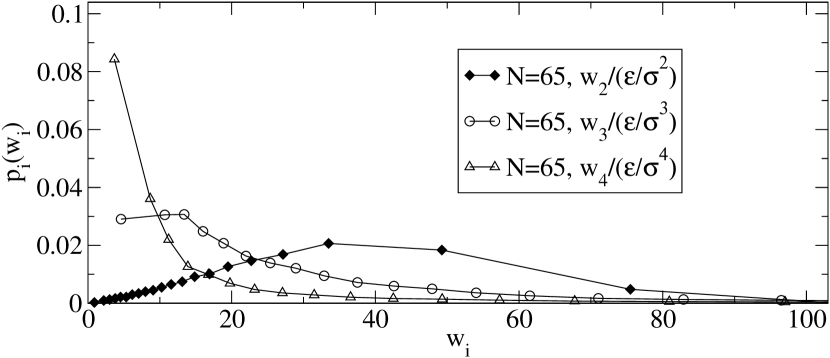
Figure 2: The $p_{i}(w_{i})$ distributions as obtained from the DWP for $N=65$.

Via a statistical procedure, as outlined in [32], we have checked that the $w_{i}$ are indeed uncorrelated.

Please note that the distribution $p_{i}(w_{i})$ is very different to the density $q_{i}(w_{i})$ which denotes the number of DWP with a given value of $w_{i}$. The reason is that the sub-volume of the $(w_{2},w_{3},w_{4})$-space which contains the DWP in the given parameter range, is highly non-trivial. Only in case that this sub-volume were a simple cube both distributions should be identical.

Based on the distributions $p_{i}(w_{i})$ it is possible to generate DWP with the correct statistics. Thus the generated DWP should have the same properties as the original DWP. This is exemplified in Fig. 1 where we show the correlations of the DWP three parameters for the original set of DWP as well as for the generated set of DWP. No relevant deviations are present. This underlines the validity of our assumption of uncorrelated $w_{i}$.

Our main goal is to generate DWP with very small asymmetry in order to obtain information about typical TLS. For perfectly symmetric DWP one has

$$w_{2}\cdot\ w_{4}/w_{3}^{2}=1/4.$$ (10)

However this relation alone does not tell which range in the $w_{2},w_{3},w_{4}$-space is relevant for nearly symmetric DWP. This question is crucial, since from Fig. 2 it is obvious that the $p_{3}$ and $p_{4}$ are ill-defined for small $w_{3}$ and $w_{4}$, respectively. Therefore in a first step we have generated DWP with $\Delta<2$K. For this subset we have calculated the $q_{i}$-distributions. They are shown in Fig. 3. On their basis it is possible to estimate which parameter range is essential for the generation of nearly symmetric DWP. Fortunately, it turns out that the range of small $w_{3}$ and $w_{4}$ is irrelevant. Thus it is indeed possible to use our original set of DWP to generate symmetric DWP, i.e. TLS with the correct statistics. This shows that the range of asymmetric DWP contains sufficient information about nearly symmetric DWP. This justified our method to use change the parameterization of the DWP by using the $w_{i}$ rather than the original parameters $(\Delta,d_{\mathrm{mwrp}},V)$.

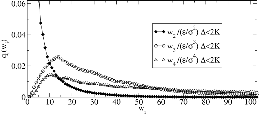
Figure 3: The distributions $q_{i}(w_{i})$ for $\Delta<2\mathrm{K}$ as calculated from the observed DWP.

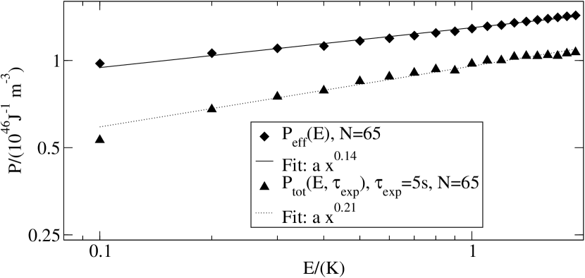
Figure 4: Energy dependency of $P_{\mathrm{eff}}$ and $P_{tot}$. The data show the weighted and unweighted cumulative number of TLS per energy and volume. Both curves can roughly be approximated by a power law.

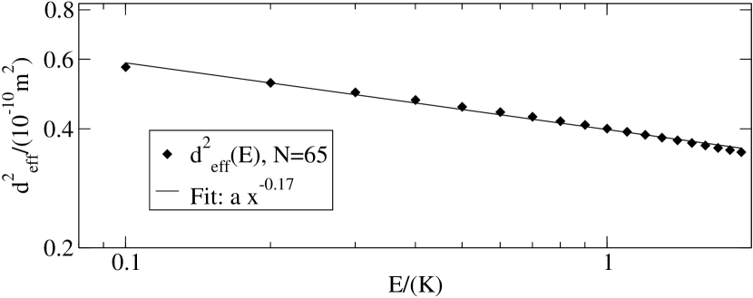
Figure 5: The effective distance decreases with higher energy splitting, because large distances correlate with a high asymmetry and low $\Delta_{0}$. The curve can roughly be approximated by a power law.

For the TLS, generated in this way, we estimate $\Delta_{0}$ with help of the Wentzel Kramer Brillouin (WKB) approximation. The validity of the one dimensional WKB approximation is discussed in [33] for the case of TLS in simulated argon clusters. They observe only minor changes in the eigenfrequencies during the transition, which makes the WKB approximation usable. We make use of the WKB approximation in a slightly different form than used by Phillips in [9]:

$$\Delta_{0}=E_{0}\cdot e^{-\frac{\pi}{4}d^{\prime}\sqrt{2\bar{m}V^{\prime}/\hbar^{2}}}.$$ (11)

Instead of approximating the barrier shape by a rectangle we used an inverted parabola. This gives the additional factor $\pi/4$ in the exponent. The primes indicate that the values have been changed by taking the harmonic ground level energies $\frac{1}{2}\hbar(2w_{2}/m)^{0.5}$ of the relevant configurations, into account, i.e. minima and saddle. This lowers the barrier height $V$ and decreases the distance $d$. By using the values for $\Delta_{0}$, $E$ and $P(\Delta_{0},\Delta)$ and according to Eqn. 6 with $E/k_{B}$ limited to 1 K we obtain $P_{eff}=1.3\pm 0.5\cdot 10^{46}\mathrm{J}^{-1}\mathrm{m}^{-3}$. This value is in good agreement with previous results [23] and the experimentally observed values for NiP [34] ($2\cdot 10^{46}J^{-1}m^{-3}$). This last value, however, might be biased by the electron contribution in NiP and is somewhat higher than commonly found values for other glass-forming systems [30], ranging from $0.5\cdot 10^{45}\mathrm{J}^{-1}\mathrm{m}^{-3}$ to $3\cdot 10^{45}\mathrm{J}^{-1}\mathrm{m}^{-3}$. In disagreement with the STM we observe an energy dependence of $P_{\mathrm{eff}}(\mathrm{E})$ which can be characterized as $P_{\mathrm{eff}}(E)\propto E^{\delta}_{1}$ with $\delta_{1}=0.14$, see Fig.4.

In the next step we compare the temperature dependence of the thermal conductivity and the heat capacity calculated from simulated TLS with experimentally found values; see Heuer and Silbey [10] for the theoretical background. The thermal conductivity is experimentally found to behave like

$$\kappa(\mathrm{T})\propto\frac{\mathrm{T}^{2}}{P_{\mathrm{eff}}\gamma^{2}_{\sigma}}\propto\mathrm{T}^{2-\beta}$$ (12)

with $\beta$ small and positive. From this and

$$P_{\mathrm{eff}}\propto\mathrm{E}^{\delta_{1}}$$ (13)

$$\gamma_{\sigma}^{2}\propto d_{\mathrm{eff}}^{2}(\mathrm{E})\propto\mathrm{E}^{\delta_{2}}$$ (14)

follows $\beta=\delta_{1}+\delta_{2}$. $d_{\mathrm{eff}}$ is defined as

$$d_{eff}^{2}(E)=\frac{\sum_{i}^{\prime}d^{2}\cdot\Delta_{i,0}^{2}/\mathrm{E}_{i}^{2}}{\sum_{i}^{\prime}\Delta_{i,0}^{2}/\mathrm{E}_{i}^{2}},$$ (15)

where the primes indicate that the sums include all TLS i with an energy splitting smaller than E. The energy dependence of $d_{eff}$ is shown in Fig. 5, yielding $\delta_{2}=-0.17$ and $\beta\approx 0.0$. For the calculation of the heat capacity experimentally limited relaxation times have to be taken into account. The heat capacity is experimentally found to be

$$\mathrm{C(T)}\propto\mathrm{T}^{1.1-1.3}.$$ (16)

For a theoretical analysis one may use the expression

$$\mathrm{C(T,\tau_{exp})}\propto\int_{0}^{\infty}\frac{P_{\mathrm{tot}}(E,\tau_{\mathrm{exp}})\mathrm{E}^{2}}{4\mathrm{k_{B}T}^{2}}sech\left[\frac{\mathrm{E}}{2\mathrm{K_{B}T}}\right]dE.$$ (17)

Here $P_{\mathrm{tot}}$ is the total number of TLS per energy and volume with energy splitting below E and with relaxation times shorter than $\tau_{\mathrm{exp}}$. For a fixed relaxation time $\tau_{\mathrm{exp}}=5s$ we obtain $P_{\mathrm{tot}}(E,\tau_{\mathrm{exp}})\propto\mathrm{E}^{1+\delta_{3}}$ with $\delta_{3}=0.21$; see Fig.4. The value of $\delta_{3}$ is not very sensitive to the exact choice of $\tau_{\mathrm{exp}}$. Inserting this relation into Eq.17 one obtains $\mathrm{C(T,\tau_{exp})}\propto\mathrm{T}^{1+\delta_{3}}$ in agreement with the experiment.

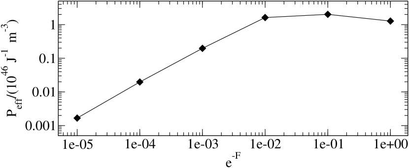
Figure 6: Dependence of the $P_{\mathrm{eff}}$ on the Franck-Condon factor. N=65, $E\approx$1 K

The comparison between experimentally determined results and simulated results has to be done with care as the tunneling matrix element is experimentally decreased by a mismatch of the vibrational modes of the two states giving rise to an additional factor [35].

$$\Delta_{0,\mathrm{exp}}=e^{-\mathrm{F}}\cdot\Delta_{0}$$ (18)

F is the Franck-Condon factor and does mainly depend on the spectral density of eigenfrequencies and their coupling to the system. The simulated number of TLS is therefore not directly comparable with experimentally determined values. To check the possible influence of $e^{-\mathrm{F}}$ on our results some values, we have calculated $P_{\mathrm{eff}}$ for different values of this factor; see Fig. 6. Interestingly, $P_{\mathrm{eff}}$ is slightly increased for $0.01<e^{-\mathrm{F}}<1$. The increase is caused by the fact that TLS with $E>1K$ are lowered in their splitting energy such that the number of TLS below 1 K is increased. For even smaller values of the Franck-Condon factor, however, the $\Delta_{0}^{2}$-factor in Eq.6 results in a significant reduction of $P_{\mathrm{eff}}$.

3.2 Microscopic Nature of the Two Level States

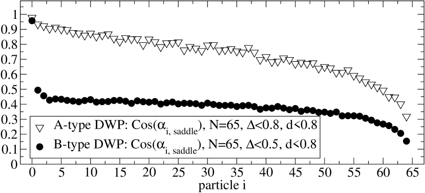
Figure 7: Cosine of the angle between the transition vector from the first minimum configuration to the saddle configuration and the vector from the saddle to the next minimum configuration. The particles are sorted according to their total motion (i=0: fastest particle). It is distinguished whether central particle is a A- (triangles) or a B-particle (spheres).

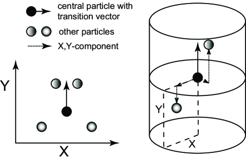
Figure 8: Sketch of the definition of the local environment of the central particle.

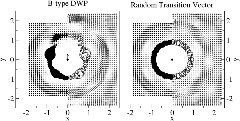
Figure 9: Left: Averaged A-particle distribution around the central B particle. The filled circles are generated from a 65 particle system and the open circles are generated from a 130 particle system. There is no visible finite size effect. Right: Same as before but with a randomly chosen transition vector for the central particle. The density distribution corresponds to the radial distribution function.

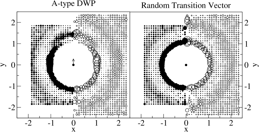
Figure 10: Same as the previous figure except that central A-particles are considered.

In our recent publication [24] we have analyzed the particle which shows the largest displacement during the transition between both minima. It is denoted central particle. DWP with an A-particle as a central particle are denoted A-type DWP. B-type DWP are defined in analogy. Surprisingly, it turned out that 90% of all DWP are B-type DWP although only 20% of all particles are B-particle. Furthermore we see that for B-type DWP the displacement of the central particles was significantly larger than that of all other particles. For A-type DWP the distribution of displacements was more continuous. Stated differently, the transition in A-type DWP is more collective.

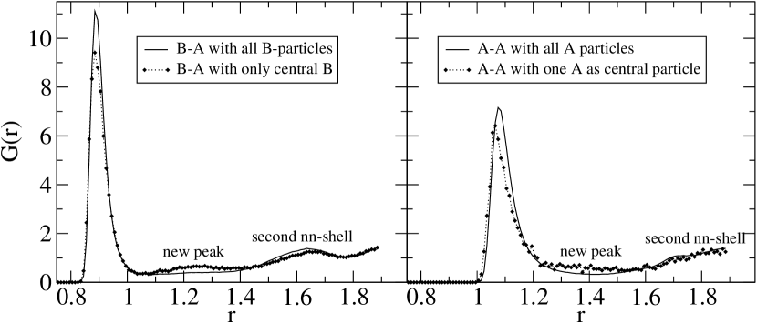
Figure 11: G(r) of the minimized structures in comparison to special G(r), where only the central particles in interaction with A-particles are considered.

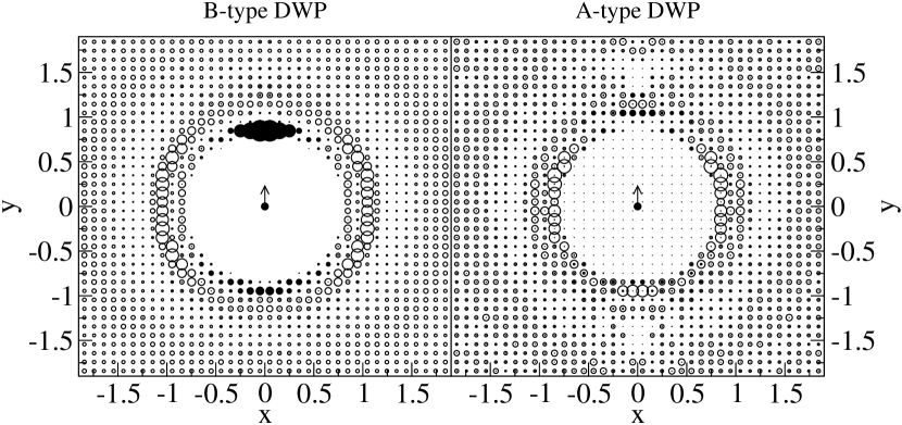
Figure 12: Particle distribution around the particle with the second-largest displacement (N=65). In analogy to Fig. 9 and Fig. 10 the transition vector of this particle defines the y-axis. The filled circles mark the contribution from the central particle.

In this subsection we elucidate the dynamics of DWP much closer. First we analyze whether the displacement between both minima is along a straight line in configuration space or whether it is curved. More specifically we calculate the angle between the transition vector from the first minimum to the saddle and from the saddle to the second minimum; see Fig. 7. The results are sorted with the respect to the displacement of the different particles (i=0: particle with the largest displacement, i.e. central particle; i=64: particle with the smallest displacement). For B-type DWP the central particle basically moves along a straight path whereas the other particles move along a strongly curved path. Thus the DWP can be basically characterized as a one-particle motion of a B-particle. The other particles just support this transition by some complicated curved trajectory to optimize the energy. The behavior is very different for A-type DWP where most particles move along a relatively straight line. Since the central particle is only little different in terms of its displacement (see above) it is not surprising that the central particle behaves similarly as compared to the other particles. Obviously, the collective dynamics in A-type DWP is realized by a rather straight translation of most particles. Note, however, that for both types of DWP there is a tendency to move in a less curved way for particles with larger displacements, even if the reaction path approximation is considered. A priori this is not a necessity.

In the next step we take a closer look into the local distribution of particles around the central particle. We therefore define the relative density in a cylinder around the central particle as shown in Fig. 8. The transition vector of the central particle defines the y-axis. Furthermore the distance vectors between the central particles and the other particles in the starting minimum are represented in the xy-plane. By taking into account appropriate phase space factors the situation of an ideal gas would correspond to a homogeneous density distribution in the xy-plane. Finally, we average over all DWP, distinguishing A-type and B-type DWP. We only consider the density of A-particles around the central particles because the B-particles are of minor statistical relevance. Fig. 9 shows the results for the B-type DWP, which dominate the investigated BMLJ-system. The first striking observation is the distinct structure (left), which is different from the average pair correlation function (right). The main structural feature is the very small density for $(\mathrm{x}\approx 0,\mathrm{y}\approx\sigma_{\mathrm{AB}}=0.88)$. This directly shows that the central B-particles moves in a direction where free space is available. An increased density in the nearest neighbor shell (nn-shell) is found orthogonal to the direction of the translation vector. Thus the central particle jumps through this structure to get to the new minimum. Note that results for N=65 and N=130 are identical within numerical uncertainties. For the larger system one can see that also the second nearest neighbor shell reflects the properties of nn-shell. On a qualitative basis the same properties are observed for A-type DWP; see Fig. 10. It is, however, much less pronounced. This is a consequence of the fact that A-type DWP are more collective.

A priori it is not clear whether this observation implies an anomalous structure around the central particle. This is checked by analyzing the radial distribution function G(r) for the average minimized structures and G(r) for the central particles of the minimized structures, see Fig. 11. We can clearly see that for both types of DWP density is taken from the first nn-shell and transferred to a new peak between the first and the second nearest neighbor shell. Thus the observed structure in the local environment does not arise from the fact that the central transition vector chooses a special direction in an average environment, but that the environment is indeed altered.

To illustrate the above observations we show a selected DWP which explicitly displays the structural patterns; see Fig. 14. Please note the particles in the intermediate shell, as well as the particles orthogonal to the transition vector.

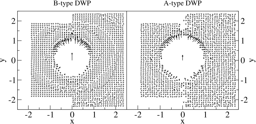
Figure 13: Averaged projected displacement of all A-particles relative to the transition of the central particle. Results for N=65 and N=130 are shown.

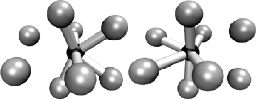
Figure 14: Type B-DWP as observed from the N=65 simulation. The small black central particle is a B-particle. The shown bonds have a length around 0.9 the non bonded atoms have a distance to the B-particle between 1.11 and 1.21. The two configurations correspond to the minima of a DWP.

To go further into structural details we repeat the analysis, performed so far for the central particle, also for the particle with the second-largest displacement. The data are presented in Fig. 12 for both types of DWP. The structural changes for the B-type DWP are dramatic if compared to Fig. 9. For the B-type DWP the first shell is almost back to normal except for an increased probability to find particles just in front of the second particle. This density is mainly caused by the central particle. This means that the particle with the second-largest displacement mainly follows the central B-particle. The A-type DWP still shows a similar picture as Fig. 10(left) but much less pronounced, the central particle shows only a small tendency to occupy positions in front of the second particle (tiny filled circles ahead of the second particle). This again is a direct consequence of the fact that for A-type DWP the central particle is not behaving very different to the other participating particles.

So far we have analyzed the structure around the central particle. In the final step we also elucidate the displacement of the particles around the central particle. The representation in Fig. 13 is analog to those in Fig. 8, the x-y-plane is still the same, but now we do not analyze where particles are in the plane but how they move relative to the central transition vector. The displacement is projected into the x-y-plane. Both graphs in Fig. 13 look similar, the differences between A- and B-type DWP are on a quantitative level. The general explanation for the observed displacements are simple. The fastest particle makes a jump from one minimum to the other and all other particles follow as if they were connected to the central particle by a spring, reflecting the attractive part of the Lennard-Jones potential.

4 SUMMARY

We were able to present a huge set of DWP, which were found on a systematic basis. The number of TLS is consistent with experimental observations and the deviations from the predictions of the STM can be explained in terms of the energy dependence of $P_{\mathrm{eff}}$ and $P_{\mathrm{tot}}$. These results were already part of older work [10] but are now reproduced on a much better statistical basis.

With the analysis of the saddle angles during the transition and the structure of the second particle we underline the single particle nature of the transition in B-type DWP, as already proposed in [24]. As the B-type DWP are predominant in the investigated BMLJ-system it follows that single particle-type DWP determine the low temperature properties of BMLJ. The more collective A-type transitions are not as important for our system but can be used as a model for other substances, where all molecules have approximately the same size and mobility.

We were also able to present a detailed analysis of the structure and the displacements of the DWP. It is shown that the presence of holes in the structure is a prerequisite for the formation of DWP. For B-type DWP one basically has a one-particle displacement. The other particles mainly follow the central particle. In contrast, for A-type DWP the dynamics are much more collective.

In a next step we aim to compare the properties with that of network glasses like silicate in order to see how the structural differences are reflected in the low-temperature properties of glasses.

References

- [1] S. Hunklinger and W. Arnold. Physical Acoustics vol. 12. ed. R. N. Thurston and W. P. Mason, New York Academic Press, 1976.
- [2] S. Hunklinger and A.K. Raychaudhuri. Progress in low temperature physics vol. IX. ed. D. F. Brewer, Elsevier, 1986.
- [3] W. A. Phillips. J. Low Temp. Phys., 7:351, 1972.
- [4] P. W. Anderson, B. I. Halperin, C. M. Varma. Phil. Mag., 25:1, 1972.
- [5] V. G. Karpov, M. I. Klinger, F. N. Ignatiev. Sov. Phys. JETP, 57:439, 1983.
- [6] U. Buchenau, Yu. M. Galperin, V. L. Gurevich and H. R. Schober. Phys. Rev. B, 43:5039, 1991.
- [7] L. Gil, M. A. Ramos, A. Bringer and U. Buchenau. Phys. Rev. Lett., 70:182, 1993.
- [8] D. A. Parshin, M. A. Ramos, A. Bringer and U. Buchenau. Phys. Rev. B., 49:9400, 1994.
- [9] W. A. Phillips. Rep. Prog. Phys., 50:1657–1708, 1987.
- [10] A. Heuer, R. J. Silbey. Phys. Rev. B, 48:9411, 1993.
- [11] D. Natelson, D. Rosenberg, D. D. Osheroff. Phys. Rev. Lett., 80:4689, 1998.
- [12] J. Classen, T. Burkert, C. Enss and S. Hunklinger. Phys. Rev. Lett., 84:2176, 1991.
- [13] D. Rosenberg, P. Nalbach, D. D. Osheroff. Phys. Rev. Lett., 90:195501, 2003.
- [14] P. Strehlow, C. Enss and S. Hunklinger. Phys. Rev. Lett., 80:5361, 1998.
- [15] S. Ludwig, C. Enss, P. Strehlow and S. Hunklinger. Phys. Rev. Lett., 70:182, 1993.
- [16] S. Kettemann, P. Fulde and P. Strehlow. Phys. Rev. Lett., 83:4325, 1999.
- [17] A. Würger, A. Fleischmann and C. Enss. Phys. Rev. Lett., 89:237601, 2002.
- [18] K. Trachenko, M. T. Dove, K. D. Hammonds, M. J. Harris and V. Heine. Phys. Rev. Lett., 81:3431–3434, 1998.
- [19] K. Trachenko, M. T. Dove, M. J. Harris and V. Heine. J. Phys.: Condens. Matter, 12:8041–8064, 1998.
- [20] T. Vegge, J. P. Sethna, S.-A. Cheong, K. W. Jacobsen, C. R. Myers and D. C. Ralph. Phys. Rev. Lett., 86:1546–1549, 2001.
- [21] H. R. Schober. J. of Non-Cryst. Solids, 307-310:40–49, 2002.
- [22] B. Doliwa and A. Heuer. Phys. Rev. E, 67:art. no. 031506, 2003.
- [23] A. Heuer, R. J. Silbey. Phys. Rev. Lett., 70:3911, 1993.
- [24] J. Reinisch and A. Heuer. arXiv:cond-mat, 0403657, 2004.
- [25] T. A. Weber and F. H. Stillinger. Phys. Rev. B, 31:1954–1963, 1985.
- [26] W. Kob and H. C. Anderson. Phys. Rev. E., 51:4626, 1995.
- [27] W. Kob. J. Phys. Condensed Matter, 11:R85, 1999.
- [28] K. Broderix, K. K. Bhattacharya, A. Cavagna, A. Zippelius and I. Giardina. Phys. Rev. Lett., 85:5360, 2000.
- [29] S. Büchner and A. Heuer. Phys. Rev. E, 60:6507, 1999.
- [30] J. F. Berret and M. Meissner. Z. Phys. B, 70:65, 1988.
- [31] A. Heuer, R. J. Silbey. Phys. Rev. B, 53:609, 1996.
- [32] A. Heuer. ed. P. Esquinazi, Tunneling Systems in Amorphous and Crystalline Solids. Springer-Verlag, 1998.
- [33] G. Daldoss, O. Pilla, G. Viliani and C. Brangian. Phys. Rev. B, 60:3200–3205, 1999.
- [34] G. Bellessa. J. Phys. (Paris), Colloq., 41:C8–723, 1980.
- [35] A. J. Legget, S. Chakravarty, A. T. Dorsey, M. P. A. Fisher, A. Garg and W. Zwerger. Rev. Mod. Phys., 59:1–85, 1987.