Orbital and spin correlations in Ca_2-xSr_xRuO₄: A mean field study

Abstract

The alloy Ca_2-xSr_xRuO₄ exhibits a complex phase diagram with peculiar magnetic metallic phases. In this paper some aspects of this alloy are discussed based on a mean field theory for an effective Kugel-Khomskii model of localized orbital and spin degrees of freedom. This model results from an orbital selective Mott transition which in the three-band system localized two orbitals while leaving the third one itinerant. Special attention is given to the region around a structure quantum phase transition at $x\approx 0.5$ where the crystal lattice changes from tetragonal to orthorhombic symmetry while leaving the system metallic. This transition yields, a change from ferromagnetic to antiferromagnetic spin correlations. The complete mean field phase diagram for this transition is given including orbital and spin order. The anisotropy of spin susceptibility, a consequence of spin-orbit coupling and orbital correlation, is a tell-tale sign of one of these phases. In the predominantly antiferromagnetic phase we describe a metamagnetic transition in a magnetic field and show that coupling of the itinerant band to the localized degrees of freedom yields an anomalous longitudinal magnetoresistance transition. Both phenomena are connected with the evolution of the ferromagnetic and antiferromagnetic domains in the external magnetic field and agree qualitatively with the experimental findings.

1 Introduction

Layered ruthenate compounds have gained an important position as a class of transition metal oxides displaying diverse physical properties. The interest in these materials has been initiated by the discovery of unconventional superconductivity in the single-layered Sr₂RuO₄ which represents most likely a realization of spin-triplet Cooper pairing, an analog of the A-phase of superfluid ³He.maeno1 ; PHYSTODAY Since the mechanism for pairing is probably of magnetic origin, the magnetic properties of related systems have been studied extensively. Increasing the number of RuO₂-layers, following through the Ruddelson-Popper series Sr_n+1Ru_nO_3n+1 with $n$ as the number of layers per unit cell, the system turns into a ferromagnet for $n\geq 3$ .CAO Peculiar metamagnetic behavior was reported for the double-layer system ($n=2$) and was interpreted as a novel type of quantum critical behavior.S3R2O7 On the other hand, replacing Sr by the isoelectronic Ca in the single-layer compound yields a Mott-insulator with antiferromagnetic long-range order of localized spin-1 degrees of freedom. These contrasting properties of the single-layer compound motivated Nakatsuji and Maeno (NM) to investigate the continuous series of alloys Ca_2-xSr_xRuO₄.NAKAMAE The interpolating phase diagram is complex. NM identified three distinct ranges of $x$ characterized by different crystal structures as well as electronic and, in particular, magnetic properties. The present study is concerned with a certain range in the NM phase diagram of these alloys (Fig.1). Therefore it is in order to briefly review here the basic experimental results for Ca_2-xSr_xRuO₄.NAKAMAE

Starting from the metallic and superconducting stoichiometric compound Sr₂RuO₄ ($x=2$) the introduction of the smaller ion Ca for Sr leads to a contraction of the crystal volume. This is achieved by the rotation of the RuO₆-octahedra, which occurs for $x<1.5$.friedt Nevertheless, up to dopings of $x=0.5$ in Ca_2-xSr_xRuO₄ the crystal structure remains tetragonal. This doping range, called region III by NM, is characterized by an increase of the uniform susceptibility which eventually becomes Curie-like with a Curie constant corresponding to nearly free spin $S=1/2$ degrees of freedom as $x=0.5$ is approached. In the doping range $0.2\leq x<0.5$, the region II following NM, the system suffers a further crystal deformation through tilting of the RuO₆-octahedra around a non-symmetric axis in the basal plane, leading to an orthorhombic crystal symmetry.friedt This results in modified magnetic properties: the Curie-like behavior is truncated, i.e. the susceptibility decreases after a pronounced maximum at low temperature. This behavior suggests antiferromagnetic correlations with a characteristic temperature scale which gradually increases, from $T\sim 0$K at $x=0.5$ to about 10 K as $x$ approaches 0.2. In addition, a pronounced inplane anisotropy in the spin susceptibility appears, indicating spin-orbit coupling effects with a two-fold symmetry axis. For both region II and III the system remains metallic. Finally, there is a first-order phase transition at $x\approx 0.2$ to a phase (region I, i.e. $0\leq x<0.2$ ) with flattened RuO₆-octahedra at low temperatures. This phase is continuously connected with the pure Ca₂RuO₆, which is a Mott-insulator and shows antiferromagnetic order with $T_{N}\sim$ 100 - 150 K. The unusual sequence of changing properties upon Ca-Sr alloying has motivated a number of theoretical studies.nomura ; terakura ; anis1 ; anis2 ; hotta

Before going into details of different attempts to explain the physics underlying these properties we discuss the basic electronic structure of the metallic Sr₂RuO₄, which is well understood experimentally as well as theoretically.BERGEMANN ; SHEN ; LDA This will be the basis for all following discussions of the alloy. The electronic band structure receives its basic character from the $4d$-$t_{2g}$ orbitals of the Ru-ion: $\{d_{yz},d_{zx},d_{xy}\}$ which disperse dominantly in each RuO₂-plane via the $\pi$-hybridization with the O-$2p$-orbitals. It is easy to see that the $d_{yz}$- and $d_{zx}$-orbitals have a very anisotropic dispersion yielding two quasi-one-dimensional bands, that hybridize to form one electron-like ($\beta$-band) and one hole-like ($\alpha$-band) Fermi surface. The quasi-one-dimensional nature of these bands produce strong nesting effects which gives rise to enhanced incommensurate spin fluctuations around a wave vector ${\bf Q}\approx(2\pi/3a,2\pi/3a,0)$ nomura ; MAZIN ; KKNG as observed in neutron scattering ($a$ being the inplane lattice constant).SIDIS The $\pi$-hybridization with the intermediate O $2p$-orbitals in both inplane directions generates for the $d_{xy}$-orbital a wider genuinely two-dimensional $\gamma$-band which has van Hove singularities rather close to the (electron-like) Fermi surface. In this way the band structure known from de Haas-van Alphen BERGEMANN and ARPES measurements SHEN is qualitatively well understood.

The doping of Ca for Sr introduces a gradual rotation of the RuO₆-octahedra around the $z$-axis and yields a modification in the band structure, which the analysis of the emerging magnetic properties in region III is based on.friedt Both groups, Nomura and Yamada (NY)nomura , and Fang and Terakura (FT)terakura , emphasize that octahedra rotation tends to narrow particularly the $\gamma$-band affecting the band structure in a way that the $\gamma$-band van Hove singularity becomes a dominant feature for the electronic properties. This leads to an increase of the uniform spin susceptibility in the region III via the increase in density of states and the Stoner enhancement. On the other hand, octahedra tilting, as occurring in region II, tends to narrow the $\alpha$-$\beta$-bands and would shift the nesting vector ${\bf Q}=(\pi,\pi,0)$ pushing the system more towards an antiferromagnetic instability. While this scenario leads to a system with metallic behavior and an enhanced uniform susceptibility in region III, it is difficult to generate the Curie-behavior displaying apparently one localized $S=1/2$ degrees of freedom per Ru-ion. This spin size is even more surprising in view of the fact that the fully localized $4t_{2g}$-orbitals with four electrons on the $Ru^{4+}$-ion would by Hund’s rule favor a spin-1 configuration, as observed in Ca₂RuO₄. Of course, complete localization is ruled out for the system being metallic.

Figure 1: Basic schematic phase diagram of Ca_2-xSr_xRuO₄ at low temperatures (following Nakatsuji and MaenoNAKAMAE ). The region III is metallic, paramagnetic and has tetragonal crystal symmetry. The region II is metallic, at low temperature with presumably antiferromagnetic correlation and has orthorhombic symmetry. In both regions the susceptibility over a certain range of temperature is Curie-like with a spin $S=1/2$. The region I is a Mott insulator with antiferromagnetic long range order of a spin $S=1$.

In contrast to the NY and FT models based on three modified itinerant electronic bands, Anisimov et al. focused their attention on the emerging spin $S=1/2$ in the susceptibility around $x=0.5$.anis1 ; anis2 In their analysis the important feature of the RuO₆-octahedra rotation is a progressive narrowing of the bands with increased Ca-doping. Due to the different character of the three bands (the parity with respect to reflection at the basal plane is opposite for the $\alpha\beta$-orbitals and $\gamma$-orbital), electron correlation will then drive a Mott transition which is orbital selective. Since the $\alpha$-$\beta$-bands, derived from quasi-one-dimensional bands, have in Sr₂RuO₄ approximately half the width of the genuinely two-dimensional $\gamma$-band, correlation would be more effective to localize their carriers. Using LDA augmented by dynamical mean field theory (DMFT) and non-crossing approximation (NCA) Anisimov et al. demonstrated that the band narrowing can indeed lead to a redistribution of the four electrons per Ru-ion and Mott transition for the $\alpha$- and $\beta$-band.anis1 ; anis2 The two orbitals $d_{yz}$ and $d_{zx}$ absorb 3 electrons while the $\gamma$-band with one electron, although half-filled, remains metallic. The 3 electrons on the two orbitals $d_{yz}$ and $d_{zx}$ generate a localized spin 1/2 and an orbital isospin 1/2 degrees of freedom. This change of electronic properties is assumed to occur upon doping and is essentially reached when $x=0.5$ is approached. For the range $0.2<x\leq 0.5$ the magnetic properties are dominated by the combination of orbital and spin degree of freedom. While this picture results in a localized spin 1/2 per site, as observed in the spin susceptibility and leads to a slight elongation of RuO₆-octahedra ($\sim 1-2\%$) as the orbital occupation is rearranged friedt , it seems in contradiction with other measurements. Recent optical spectroscopy data do not observe as drastic a change of carrier concentration in the range $0.5<x<0.9$ as one would anticipate from an orbital-selective Mott transition.LEE Furthermore, an apparent inconsistency in the orbital structure has been reported based on neutron scattering data.NEW-BRADEN Recently, Liebsch argued based on a modified DMFT approach that orbital-selective Mott transition is unlikely to occur for the $4d-t_{2g}$-orbitals.liebsch However, Koga et al. have very recently demonstrated that under rather general conditions an orbital-selective Mott transition in a two-band Hubbard model is possible, contradicting Liebsch’s argument KOGA .

Despite the mentioned reservation towards the orbital-selective Mott transition we will use this scenario in this paper as a working hypothesis and investigate some possible consequences mainly for the region II of the NM phase diagram. We find properties of the model which are in surprisingly good qualitative agreement with important features experimentally observed. Assuming three localized electrons in the $d_{yz}$-$d_{zx}$-orbitals we discuss the effective Kugel-Khomskii-type Hamiltonian describing the corresponding localized degrees of freedom, spin and orbital isospin, within a mean field theory. Including doping disorder into the model gives an important clue for the comparison with experimental findings. In particular, it allows to discuss the observed metamagnetic transition and the unusual magnetoresistance behavior in region II. We will conclude that the picture of localized $d_{yz}$-$d_{zx}$-orbitals gives a good description of the magnetic properties of the region II which is probably difficult to explain with only itinerant electrons in all three orbitals.

2 Effective Kugel-Khomskii Model

For doping concentrations $x$ in region II and at the boundary of III the $d_{yz}$-$d_{zx}$-orbitals are considered to be localized, according to Anisimov et al..anis1 ; anis2 We now introduce an effective model for these localized orbitals, and will neglect the still itinerant $\gamma$-band (which will play a role again in a later stage). This is obviously a drastic simplification in view of the influence the $\gamma$-band may have on the two localized orbitals. There are two basic types of coupling: (1) RKKY-interaction and (2) double exchange. The former tends towards an antiferromagnetic spin correlation, while the latter, in contrast, would prefer ferromagnetism. Despite the fact that the $\gamma$-band is half-filled, the band structure is far from particle-hole symmetric, so that no dangerous singular features in the RKKY coupling would appear. Thus it is unclear which trend would win. We shelve this problem for the following discussion, acknowledging the short-coming of in our simplified model. The considerably more complex complete model will be a matter of future study.

The three localized electrons in the two orbitals ($d_{zy},d_{zx}$) create four different configurations, consisting of a spin 1/2, $|\uparrow\rangle$ and $|\downarrow\rangle$, and an orbital degree of freedom, $|+\rangle$ and $|-\rangle$ describing the singly occupied $d_{zx}$ and $d_{yz}$, respectively. Analogous to the spin also the orbital degree of freedom corresponds to a two-dimensional SU(2)-symmetric Hilbert space represented by an isospin. We define, therefore, isospin operators ${I}$ which act in the following way

$$I^{z}|\pm\rangle=\pm\frac{1}{2}|\pm\rangle,\qquad I^{+}|-\rangle=|+\rangle,\qquad I^{-}|+\rangle=|-\rangle\;.$$ (1)

Hence, on every site the localized state consists of a set of four product states

$$\{|\uparrow+\rangle,\;|\uparrow-\rangle,\;|\downarrow+\rangle,\;|\downarrow-\rangle\}.$$ (2)

The fundamental microscopic model providing the dynamics for these degrees of freedom is an extended two-orbital Hubbard model (neglecting the $\gamma$-band) where we restrict ourselves to nearest-neighbor hopping and onsite interaction for the intra- and inter-orbital Coulomb repulsion, $U$ and $U^{\prime}$, respectively, and the Hund’s rule coupling $J_{H}$.

$$\begin{array}[]{ll}{\cal H}_{\alpha,\beta}=&\displaystyle-t\sum_{i,{\bf a},s}\{c_{i+a_{y},yz,s}^{{\dagger}}c_{i,yz,s}+c_{i+a_{x},yx,s}^{{\dagger}}c_{i,zx,s}+h.c.\}\\ &\\ &\displaystyle-\mu\sum_{i,s,\nu}c_{i,\nu,s}^{{\dagger}}c_{i,\nu,s}\\ &\\ &\displaystyle+U\sum_{i}\sum_{\nu}n_{i\nu\uparrow}n_{i\nu\downarrow}+U^{\prime}\sum_{i}n_{i,zx}n_{i,yz}\\ &\\ &\displaystyle+J_{H}\sum_{i,s,s^{\prime}}c_{i,yz,s}^{{\dagger}}c_{i,zx,s^{\prime}}^{{\dagger}}c_{i,zx,s}c_{i,yz,s^{\prime}}\;,\end{array}$$ (3)

where $c_{m,i,s}^{{\dagger}}$ ($c_{m,i,s}$) creates (annihilates) an electron on site $i$ with orbital index $\nu$ ($=yz,zx$) and spin $s$ ($n_{i,\nu,s}=c_{i,\nu,s}^{{\dagger}}c_{i,\nu,s}$, $n_{i,\nu}=n_{i,\nu,\uparrow}+n_{i,\nu,\downarrow}$; ${\bf a}=(a_{x},a_{y})=(1,0)$ or $(0,1)$ basis lattice vector). The effective nearest-neighbor Hamiltonian in terms of spin and isospin has the form of a Kugel-Khomskii model and can be derived within second order perturbation in $t/U$,

$${\cal H} = J\sum_{i,{\bf a}}\left[\left\{A(I^{z}_{i+{\bf a}}+\eta_{{\bf a}})(I^{z}_{i}+\eta_{{\bf a}})+B\right\}{\bf S}_{i+{\bf a}}\cdot{\bf S}_{i}\right.$$ (4)

$$\left.+[C(I^{z}_{i+{\bf a}}+\eta^{\prime}_{{\bf a}})(I^{z}_{i}+\eta^{\prime}_{{\bf a}})+D\right]$$

with the coefficients

$$A = \frac{3\alpha^{2}+1}{(3\alpha-1)(\alpha+1)}$$ (5)

$$B = \frac{-(1-\alpha)^{2}}{(3\alpha^{2}+1)(3\alpha-1)(\alpha+1)}$$ (6)

$$C = \frac{5-3\alpha}{4(3\alpha-1)}$$ (7)

$$D = \frac{1}{(5-3\alpha)(3\alpha-1)}$$ (8)

$$\eta_{{\bf a}} = \frac{(3\alpha-1)(\alpha+1)}{2(3\alpha^{2}+1)}(a_{x}^{2}-a_{y}^{2})$$ (9)

$$\eta^{\prime}_{{\bf a}} = \frac{3\alpha-1}{2(5-3\alpha)}(a_{x}^{2}-a_{y}^{2})$$ (10)

where $\eta_{{\bf a}}$ and $\eta^{\prime}_{{\bf a}}$ have opposite sign for the $x$- and $y$-axis bonds. We impose the (approximatively valid) relation $U=U^{\prime}+2J_{H}$ with $\alpha=U^{\prime}/U$ and $J=4t^{2}/U$. In order to obtain a valid approximation $\alpha$ should lie between 1/3 and 1, and not too close to these boundary values. We choose throughout this paper $\alpha=3/4$ as a representative value whenever we do a concrete analysis of this model. We emphasize that while the spin has complete SU(2) symmetry, the isospin has only Ising-like interactions, i.e. quantum fluctuations are suppressed for the latter.

The Hamiltonian (4) describes the system with tetragonal crystal symmetry corresponding to regime III in the experimental phase diagram close to $x=0.5$. Now we add terms which describe the orthorhombic distortion due to the tilting of the octahedra with the rotation axis in the basal plane. We do not speculate about the origin of this lattice deformation, which we consider to lie outside our model. Following Ref. anis2 we introduce these with the strains $\epsilon_{1}=\epsilon_{xx}-\epsilon_{yy}$ corresponding to a rotation axis like [100] and $\epsilon_{2}=\epsilon_{xy}$ corresponding to the axis [110]. These distortions lift the orbital degeneracy of $(d_{yz},d_{zx})$ and, hence, can be viewed as an effective “uniform field” polarizing the isospins in a certain direction. From symmetry considerations it follows that

$${\cal H}_{dist}=\sum_{i}[K_{1}\epsilon_{1}I^{z}_{i}+K_{2}\epsilon_{2}I^{x}_{i}]$$ (11)

where $K_{1,2}$ are coupling constants (see the Appendix). The first term is a longitudinal field while the second term corresponds to a transverse field, introducing quantum fluctuations. In connection with the Ising Hamiltonian (4) this second term provides the possibility of a continuous quantum phase transition.sachdev The lattice distortion in the regime II has a tilt axis lying between [100] and [110], so that both strains are turned on, if the border at $x=0.5$ between the two phases is crossed.

3 Mean field approximation

We now discuss the basic properties of this model and its phase diagram within a mean field approximation for both the spin and isospin degree of freedom. The Hamiltonian on the square lattice possesses a bipartite structure, which is the basis of our mean field decoupling. We introduce different mean fields for the corresponding $A$- and $B$-sublattice.

$$\langle I^{z}_{i}\rangle=\left\{\begin{array}[]{ll}t_{A}&i\in A\\ t_{B}&i\in B\end{array}\right.\quad\mbox{and}\quad\langle S_{i}^{z}\rangle=\left\{\begin{array}[]{ll}s_{A}&i\in A\\ s_{B}&i\in B\end{array}\right.$$ (12)

The mean field calculation is straightforward, whereby the self-consistent equations are solved numerically. We find the following properties.

3.1 Tetragonal system

First we consider the situation in the absence of any orthorhombic strains, $\epsilon_{1}=\epsilon_{2}=0$. For the choice of parameters ($\alpha=3/4$) we find that the coupling of the isospins, represented by $JC$, has a higher energy scale than the one for the spins, leading to a higher mean field transition temperature. The parameter $C$ in Eq.(4,7) is positive, favoring a staggered (Ising-antiferro-) orbital order. This orbital order implies ferromagnetic exchange between the spins. Note that this gives rise to enhanced uniform spin susceptibility as observed in experiment. The transition temperature to ferromagnetic order is low compared to the energy scale of the orbital order, so that it is natural to expect over a wide range of temperature a Curie-like susceptibility originating from almost independent spin 1/2 degrees of freedom, consistent with the experimental observation.

3.2 Orthorhombic distortion

Now the uniaxial strains $\epsilon_{1}$ and $\epsilon_{2}$ are turned on. Since in regime II the crystal symmetry is determined by the rotation of the octahedra around an inplane axis which does not coincide with a crystal symmetry axis, both strains, $\epsilon_{1}$ and $\epsilon_{2}$ appear. For our calculations we assume that $K\epsilon_{1}=0.75K\epsilon_{2}=K\epsilon$ which we use as a control parameter for our phase diagram. Let us first consider the orbital part only, ignoring the spin part. We observe a competition between the staggered order and the uniform alignment induced by the strain field. The transverse isospin component $I^{x}$ induced by the strain $\epsilon_{2}$ reduces the transition temperature, driving the system towards a quantum phase transition. This is included in our mean field approach with the following self-consistence equations.

$$\begin{array}[]{ll}t_{A}=&\displaystyle-\frac{2JCt_{B}+K_{1}\epsilon_{1}}{2\sqrt{(2JCt_{B}+K_{1}\epsilon_{1})^{2}+K_{2}^{2}\epsilon_{2}^{2})}}\\ &\\ &\displaystyle\times\tanh\left(\beta\sqrt{(2JCt_{B}+K_{1}\epsilon_{1})^{2}+K_{2}^{2}\epsilon_{2}^{2})}\right).\end{array}$$ (13)

The isospin component $t_{x}=\langle I^{x}\rangle$ is obtained as

$$\begin{array}[]{ll}t_{xA}=&\displaystyle-\frac{K_{2}\epsilon_{2}}{2\sqrt{(2JCt_{B}+K_{1}\epsilon_{1})^{2}+K_{2}^{2}\epsilon_{2}^{2})}}\\ &\\ &\displaystyle\times\tanh\left(\beta\sqrt{(2JCt_{B}+K_{1}\epsilon_{1})^{2}+K_{2}^{2}\epsilon_{2}^{2})}\right)\end{array}$$ (14)

for the $A$-sublattice site. The analogous expressions for the $B$-sublattice site are obtained by exchanging $t_{B}$ and $t_{A}$ in these equations. The $t_{x}$-component is only finite, if the orthorhombic strain $\epsilon_{2}$ is present.

Figure 2: Mean field phase diagram as a function of temperature $T$ and strain $K\epsilon$. Thin lines denote second order phase transitions and the thick line a first order phase transition.

The staggered orbital moment $t_{s}=(t_{A}-t_{B})/2$. Increasing the strains leads to a gradual diminishing of $t_{s}$ and the corresponding transition temperature until it would vanish at a quantum critical point. In turn the mean fields $(t_{xA}+t_{xB})/2$ and $t_{0}=(t_{A}+t_{B})/2$ increase continuously favoring AF spin correlation resulting in the phase diagram shown in Fig. 2. The decrease of $t_{s}$ leads at the same time to a weakening of the ferromagnetic correlation and the gradual increase of a uniform isospin correlation gives rise to a competing antiferromagnetic spin correlation. Indeed the continuous evolution of $t_{s}$ is truncated by the onset of antiferromagnetic spin order, before the anticipated quantum suppression of the staggered isospin order is completed. This spin correlation is favored by the strain driven ferro-orbital correlation and has a higher energy scale (mean field transition temperature) than the ferromagnetic order. Consequently, the staggered isospin phase and the antiferromagnetic order are separated by a first order transition. There is even a reentrant behavior associated with this first order instability such that around a critical range of $K\epsilon\approx 0.5J$ upon lowering temperature first a staggered isospin phase with enhanced tendency towards ferromagnetism would be reached and with a first order transition (thick line in Fig. 2) at lower temperature the antiferromagnetic phase would appear. Otherwise all phase transitions in the phase diagram of Fig. 2 are second order (thin lines).

The evolution of the system, under orthorhombic distortion, from ferromagnetic towards antiferromagnetic behavior displays the correct qualitative trend in comparison with the experimental situation. The fact that the temperature scale of the antiferromagnetic state is higher than that of the ferromagnetic is also in qualitative agreement with experimental data. The former is easily visible in experiment at a temperature $T\sim 5-10K$ around $x=0.2$, while the latter can brought into connection with a irreversibility transition observed in the vicinity of $x=0.5$ below $\sim 1K$.SUGAHARA The irreversibility and the sensitivity to slow dynamics led to the interpretation as a cluster glass. Similar features could arise in an inhomogeneous ferromagnetic phase.SUGAHARA

3.3 Spin-orbit coupling and anisotropic spin susceptibility

For the Ru-ion spin-orbit coupling is not negligible. The microscopic formulation of spin-orbit coupling involves the whole set of $t_{2g}$-orbitals including the itinerant $\gamma$-orbital.kong We remain within our present reduced model and restrict ourselves to a phenomenological approach where the effect of spin-orbit coupling enters via the $g$-tensor modifying the Zeeman term in the Hamiltonian. This term can be derived from symmetry considerations analogous to the coupling of the strain (Appendix A).

$$\begin{array}[]{l}\displaystyle{\cal H}_{Z}=-\mu_{B}\sum_{i}[g{\bf H}\cdot{\bf S}_{i}+g_{1}\langle I^{z}_{i}\rangle(H_{x}S^{x}_{i}-H_{y}S^{y}_{i})\\ \\ \displaystyle\qquad\qquad+g_{2}\langle I^{x}_{i}\rangle(H_{x}S^{y}_{i}+H_{y}S^{x}_{i})]\end{array}$$ (15)

where only the two isospin directions $I^{z}$ and $I^{x}$ have been included, ignoring $I^{y}$ which is not induced by strain nor interaction ($\mu_{B}$: Bohr magneton). Two coupling constants $g_{1}/g$ and $g_{2}/g$ enter as phenomenological parameters. $\langle I^{a}\rangle$ denotes the average of the orbital configurations on all sites. Here we want to concentrate on the anisotropy of the susceptibility in the basal plane ($x$-$y$) which shows the most distinguished effect.

We now calculate the spin-susceptibility on the background of the staggered orbital order and the driven ferro-orbital correlation:

$$\chi(T,\phi)=\chi_{0}(T)\{1+\frac{g_{1}}{g}\langle I^{z}\rangle\cos 2\phi+\frac{g_{2}}{g}\langle I^{x}\rangle\sin 2\phi\}$$ (16)

where the angle corresponds to the orientation of the field in the basal plane relative to the $x$-axis. The isotropic susceptibility $\chi_{0}(T)$ includes the spin correlation and approaches the behavior of free spins for temperatures much higher than the Neél temperature in our model.

In the tetragonal phase where a staggered Ising orbital order is realized the average of the isospin vanishes and, consequently, there is no basal plane anisotropy in the spin susceptibility. This is fully consistent with the experiment at $x=0.5$. On the other hand, the orthorhombic distortion which yields polarized orbitals in region II gives rise to anisotropy. Let us for simplicity now assume that the orthorhombic distortion is of the type $\epsilon_{xy}\neq 0$ and $\epsilon_{xx}-\epsilon_{yy}=0$. Hence we find that only $\langle I^{x}\rangle\neq 0$. If the temperature is much higher than the characteristic energy scale for the orbital correlation, the isospin can be approximately considered as an independent degree of freedom in a driving field, i.e. $\langle I^{x}\rangle\approx K_{2}\epsilon_{xy}/4k_{B}T$. Here we assume that the strain $\epsilon_{xy}$ only weakly depends on temperature and keep it constant. This is only valid far away from the phase boundary of the structure phase transition. Thus, the anisotropy of the spin susceptibility can be described by the ratio of the maximal to minimal value

$$\frac{\chi(\pi/4)}{\chi(-\pi/4)}=\frac{g+g_{2}\langle I^{x}\rangle}{g-g_{2}\langle I^{x}\rangle}\approx\frac{4gk_{B}T+K_{2}\epsilon_{xy}g_{2}}{4gk_{B}T-K_{2}\epsilon_{xy}g_{2}}$$ (17)

which tends to 1 for large temperatures and grows for decreasing temperatures. Obviously the anisotropy increases too, if $\epsilon_{xy}$ becomes larger, which implies a growing anisotropy for samples with $x\to 0,2$ in region II. For a qualitative view of the behavior we plot for different parameters $K_{2}\epsilon_{2}$ (Fig.3). This behavior is close to the observed one by NM.NAKAMAE

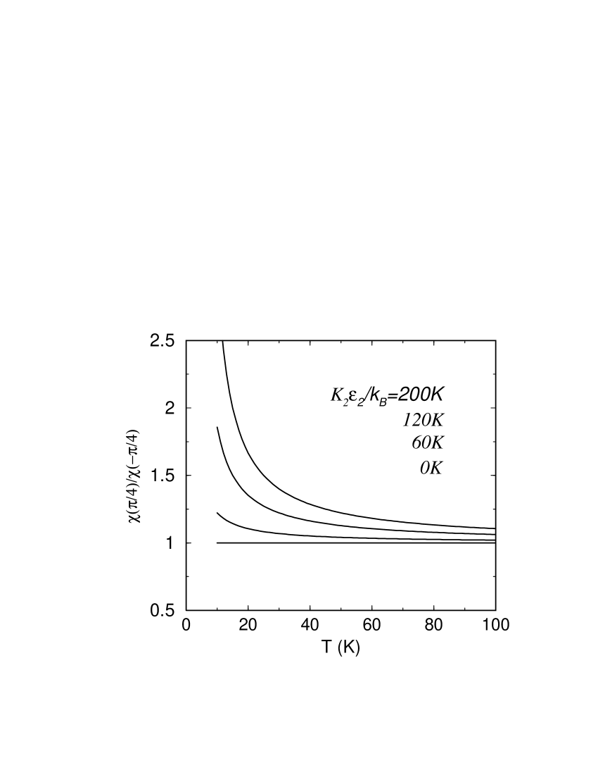
Figure 3: Anisotropy of susceptibility: Ratio of the maximal and minimal susceptibility as function of temperature for $g_{2}/g=0.1$ and different levels of distortion $K_{2}\epsilon_{2}$.

4 Effects of an external magnetic field and alloy inhomogeneity

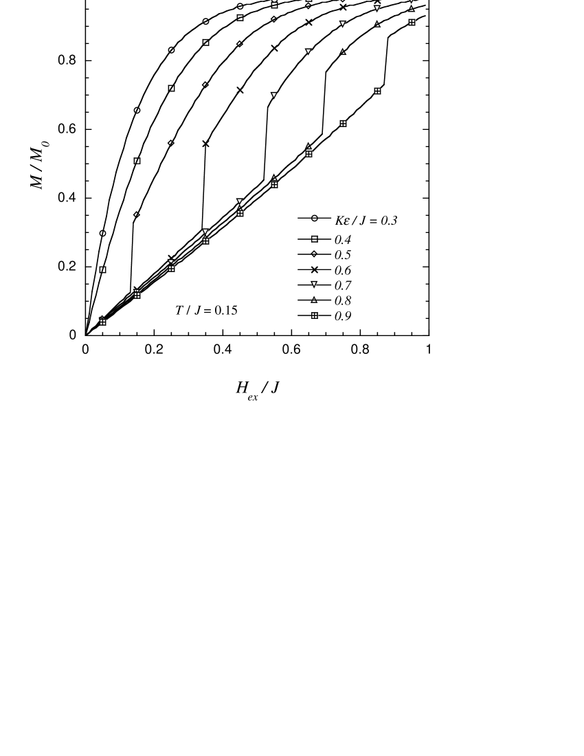
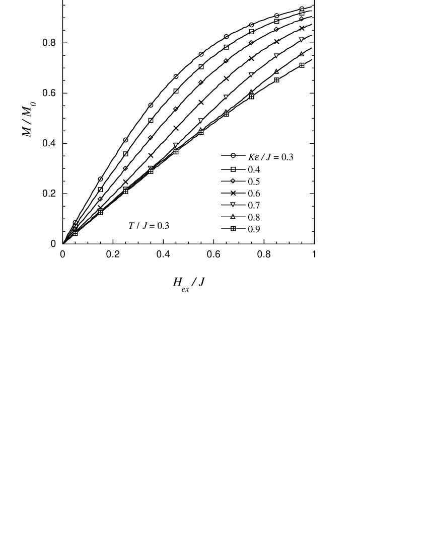
Figure 4: Magnetization curves at three temperatures for different values of $K\epsilon/J$.

We focus now on the phase in which the lattice distortion induces the FO-order and AF-spin order. Close to the first-order phase transition line the phase with a staggered orbital order and the ferromagnetic spin correlation forms a metastable states. This can be stabilized by an external magnetic field, since the antiferromagnetic phase has a lower uniform spin susceptibility. A discontinuous “metamagnetic” transition appears, since the magnetic field allows us to traverse the first-order phase transition line and to reach the phase of higher magnetization. This type of transition had been investigated in another context by Khomskii and Kugel KK . In our mean field calculation we apply the magnetic field along the $z$-axis and introduce two additional mean fields $s_{xA}$ and $s_{xB}$ as order parameters of the antiferromagnetic order perpendicular to the field, in addition to the uniform component along the field. In Fig. 4 we show the mean field results of the magnetization curves for three temperatures and a series of distortion strengths. For low temperature indeed a discontinuous transition between a low and high magnetization state is found. Obviously, this transition would be hysteretic since it is first order. Obviously, the field-induced first-order transition leads to a rearrangement of the orbitals and should result in a structural deformation as well KK .

4.1 Metamagnetic transition

The real material does not exhibit a discontinuous metamagnetic transition even at low temperatures. The short-coming in our model lies in the assumption of homogeneity. Obviously, the random alloy would rather have spatial fluctuations, for example, in the crystal deformation field $K\epsilon$. A spatial variation of $K\epsilon$ would give rise to the appearance of both the antiferromagnetic and the staggered orbital phase with ferromagnetic spin fluctuations in form of domains. They are separated by rather sharp domain boundaries, if the randomness is sufficiently broad and smooth.YMRI We distinguish $A$- and $F$-domains which denote the domains with antiferromagnetic and ferromagnetic spin correlation, respectively. We consider a system where the antiferromagnetic phase dominates and the F-domains form at most small islands, as would be likely the case for $x\approx 0.2$ based on our model. These $F$-islands develop a magnetic moment at low temperature once the ferromagnetic correlation length reaches their spatial extension. In turn the moments of different islands are correlated via the antiferromagnetically correlated background. This effective interaction may be frustrating so that under certain conditions at low enough temperature even glass-like behavior can occur. We will here, however, concentrate on the behavior under a magnetic field.

The external magnetic field $H_{ex}$ polarizes the magnetic moments of both domains. Because the F-domains possess the larger susceptibility, their free energy density drops more rapidly with increasing field than that of the A-domains. Thus the F-domains grow at the expense of the A-domains. The initial linear response of the magnetization to the field turns nonlinear, if the domains change their size. In this way the metamagnetic transition, which was discontinuous and hysteretic in the homogeneous system, would be smeared, continuous and reversible for the inhomogeneous case.YMRI The inflection point of the magnetization as a function of $H_{ex}$, would roughly correspond to the highest density of the domain boundaries through the system, because this yields the most rapid change of the domain sizes as a function of $H_{ex}$. The metamagnetic transition lies, consequently, also rather close to the point where the domain boundaries percolate throughout the sample.

4.2 Extended mean field approach

The continuous metamagnetic behavior of the inhomogeneous system can be very easily simulated within our mean field calculation. We modify Eq.(11) to a random field coupling

$${\cal H}_{dist}=\sum_{i}[K_{1}\epsilon_{1i}I^{z}_{i}+K_{2}\epsilon_{2i}I^{x}_{i}]$$ (18)

so that for every site, in principle, the crystal field may be different. Since one has to consider certain realizations of randomness we can only deal with finite lattices. We use a lattice size of $100\times 100$ to simulate the evolution of the domain distribution in a magnetic field. For this purpose the model was set up in the following way. In order to obtain a smoothly varying distribution we start with an uncorrelated uniform distribution of random numbers in the interval $[-0.9,2.7]$ Averaging the values five times with the values at the four nearest neighbor sites we finally arrive at a smooth distribution shown in Fig. 5, with mean value $\overline{K\epsilon}/J=0.9$ and with a standard deviation $\Delta K\epsilon/j=0.2$, correlated over several lattice sites.

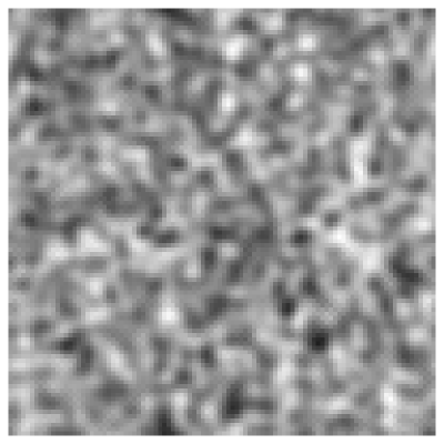
Figure 5: Distribution of $K\epsilon/C$ used in the mean field calculation. The mean value of $K\epsilon/C$ is $0.9$ and the standard deviation $0.2$. Black corresponds to the minimum value of 0.2 and white to the maximum value of 1.6

For the mean field calculation we start from an initial configuration that has staggered orbital order for the $t_{z}$ mean fields, uniform magnetic order for the $s_{z}$ mean fields in the direction of the magnetic field and staggered antiferromagnetic order for the $s_{x}$ mean fields perpendicular to the magnetic field. In order to find a zero-temperature mean field solution we then perform $10^{6}$ updates to this mean field, solving the mean field equations each time for one randomly chosen spin, using a quantum operator library developed by one of the authors QET .

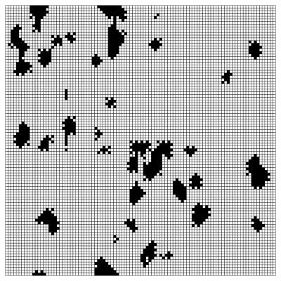
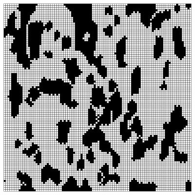
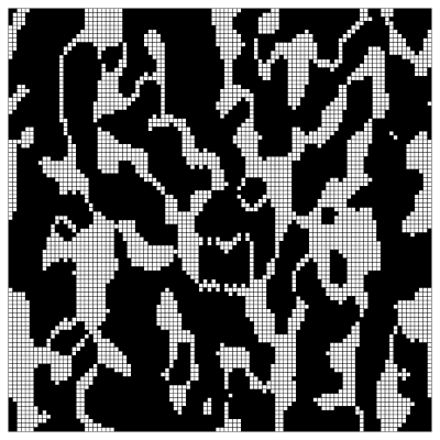
Figure 6: Distribution of ferromagnetic (black) and antiferromagnetic (white) domains at a) a weak field $h/J=0.2$ and b) close to the percolation threshold with $h/J=0.3$ and c) at stronger fields $h/J=0.4$.

Since most of the $K\epsilon$ values are inside the antiferromagnetic phase we find only small islands of staggered orbital order and ferromagnetism (Fig. 6a). Increasing the fields we can observe that these ferromagnetic domains grow, and percolate at a “transition” to a ferromagnetic phase (Fig. 6b,c). This transition is accompanied by a smooth metamagnetic like magnetization curve, shown in Fig. 7a. The volume of the F-domains grow monotonically as shown in Fig.7b.

We would like to mention here that the presence of a metamagnetic transition has been observed in region II naka-phd ; SUGAHARA . Also a structural response has probably be seen in experiment FRIEDT2 .

Figure 7: Zero temperature magnetization curve and volume fraction of the ferromagnetic domain of the inhomogeneous system with the distribution of Fig. 5.

4.3 Phenomenological model

We now illustrate the result of our mean field simulation by means of a simple phenomenological model describing the distribution of the F- and A-domains. We define the free energy at a given temperature as

$$F(l;H_{ex},T) = \frac{W}{2}(l-l_{0})^{2}-V_{F}(l)f_{F}(H_{ex},T)-$$ (19)

$$V_{A}(l)f_{A}(H_{ex},T),$$

where we denote the integrated area of the F- and A-domains by $V_{F}(l)$ and $V_{A}(l)$ (note $V_{F}+V_{A}=V$ the total area), and $l$ is a variable determining the domain distribution. It is chosen so that the energy expense by deviating from the zero-field equilibrium state (characterized by $l=l_{0}$) follows the quadratic behavior with an “elastic constant” $W$. Increasing $l>l_{0}$ leads to the enlarging of $V_{F}(l)$ which is a monotonically growing function of $l$. The free energy densities in the two domains are denoted as $f_{F}$ and $f_{A}$ and are a function of the field.

The equilibrium value of $l$ for a given external field $H_{ex}$ is obtained by minimizing the free energy. This leads to the equation

$$W(l-l_{0})+[f_{F}(H_{ex},T)-f_{A}(H_{ex},T)]\nu(l)=0$$ (20)

with

$$\nu(l)=\frac{\partial V_{F}}{dl}(l),$$ (21)

a measure for the density of domain boundaries. It is obvious that $\nu(l)$ would be non-monotonic with a maximum at an intermediate value of $l$. The integral $\int dl\nu(l)$ running from $l=-\infty$ to $+\infty$ gives the total volume $V$. This function characterizes the inhomogeneous system within this theory. Since $f_{F}<f_{A}$ in a finite field the solution of Eq.(20) yields $l(H_{ex})$ as a monotonically growing function of $H_{ex}$. The magnetization of the system is given by

$$\begin{array}[]{ll}\displaystyle M=-\frac{dF}{dH_{ex}}&\displaystyle=-V_{F}(l)\frac{df_{F}}{dH_{ex}}+(V-V_{F}(l))\frac{df_{A}}{dH_{ex}}\\ &\\ &=V_{F}(l)M_{F}+(V-V_{F}(l))M_{A}\;.\end{array}$$ (22)

We use the following simple approximative forms for the free energy densities in a magnetic field:

$$f_{a}(H_{ex},T)=f_{0a}-\frac{M_{0a}^{2}}{\chi_{0a}}{\rm ln}\cosh(\chi_{0a}H_{ex}/M_{0a})$$ (23)

with $a=F,A$ and $f_{0a}=f_{a}(0)$ ($f_{0F}=f_{0A}$). Here $M_{0a}$ is the saturation moment and $\chi_{a0}$ is the uniform spin susceptibility in the linear response regime at the given temperature $T$. Thus, the magnetization is given by

$$M_{a}=-\frac{df_{a}}{dH_{ex}}=M_{0a}\tanh(\chi_{0a}H_{ex}/M_{0a})$$ (24)

Note that in this discussion we do not rely on the presence of long range order, neither FM nor AFM. The characteristic function $\nu(l)$ depends on the specific realization of the alloy. We may take as a simple example

$$\nu(l)=\frac{V}{2{\rm arctan}(\tilde{l})}\frac{L}{l^{2}+L^{2}}$$ (25)

for $|l|<\tilde{l}$ and $\nu(l)=0$ otherwise and $-\tilde{l}<l_{0}<0$. Eq.(20) can solved numerically. For a given set of parameters we display the results in Fig. 8. In Fig. 8a) the volume of the F-domains as a function of $H_{ex}$ is shown to grow monotonously and in Fig. 8b) the magnetization exhibits a clear metamagnetic transition at the point of fastest change of the volume.

4.4 Longitudinal Magnetoresistance

We now would like to consider the effect of domains on the transport in the metallic $\gamma$-band which we had neglected so far. Naturally the conductance of the $\gamma$-band depends also on the correlation of the localized degrees of freedom of the $\alpha$-$\beta$-orbitals, since they interact via onsite couplings, such as Hund’s rule coupling. First of all the two uniform phases A and F would have slightly different electrical conductance, $\sigma_{A}$ and $\sigma_{F}$. For the inhomogeneous phase the domain boundaries also play a role. They are restricted regions where orbital and spin degrees of freedom have a rapid spatial dependence connecting the two kinds of domains, so that the scattering of electrons of the $\gamma$-band in the domain boundary region is enhanced. This readily understood from the point of view that the A- and F-domains in a magnetic field have different magnetizations. Thus the rapid change of magnetization in the domain boundary constitutes a scattering potential.

Figure 8: Results of the phenomenological model: a) Volume of the F-domain; b) magnetization ; c) longitudinal magnetoresistance. Parameters: $W=0.1V$, $L=2$, $l_{0}=2$, $\tilde{l}=2.5$, $M_{0F}=M_{0A}=1$, $\chi_{OF}=0.3$ and $\chi_{0A}=0.02$.

We would like to consider the problem of the longitudinal magnetoresistance, i.e. the resistance for a current which flows parallel to the applied external (inplane) field. The change of the domain distribution is the key ingredient determining the field dependence of the resistance. We address this problem again from the point of view of our simple phenomenological model. The overall conductance of the sample neglecting the domain boundaries may be roughly approximated by the averaged conductance

$$\bar{\sigma}=\frac{V_{F}\sigma_{F}+(V-V_{F})\sigma_{A}}{V}.$$ (26)

if the conductances $\sigma_{F}$ and $\sigma_{F}$ have comparable magnitude. Next we introduce the effect of the domain boundaries. As additional scattering regions their influence depends on their density. Hence, the resistance contains two parts coming from the domains and the domain boundaries:

$$\rho=\frac{1}{\bar{\sigma}}+\tilde{\rho}.$$ (27)

Here $\tilde{\rho}$ denotes the domain boundary part which we approximate as proportional to the density of boundaries, corresponding to $\nu$: $\tilde{\rho}=\rho_{0}\nu$. Now we can discuss the field dependence of $\rho$ by inserting the solution of Eq.(20), $l(H_{ex})$. This leads to a sensible qualitative behavior of the longitudinal magnetoresistance as can be seen in Fig.8c) showing $\Delta\rho(H_{ex})=\rho(H_{ex})-\rho(0)$. There is a pronounced maximum at essentially the same position as the metamagnetic transition occurs, both connected with the domain boundary percolation condition. It is also worth noting that the low-field limit leads to

$$\Delta\rho(H_{ex})\propto l-l_{0}\propto f_{F}(H_{ex})-f_{A}(H_{ex})\propto H_{ex}^{2}.$$ (28)

This low-field behavior and the overall field dependence compares well with the experimental data by NM.nakatsu ; naka-phd In the experiment a pronounced maximum is found at approximately the field corresponding to the metamagnetic transition. This strong feature in the magnetoresistance disappears for temperature higher than the characteristic temperature of the antiferromagnetic spin correlation ($\sim 10K$). Naturally the domain formation is absent when there is no spin correlation (AFM order in our mean field treatment).

4.5 Resistor network approach

The issue of transport in such a system is naturally complex since it involves percolation of domains and domain boundaries. This aspect is not taken into account in our model where we the domain boundaries only considered as additional uncorrelated scatterers entering the resistance only through their density. The domain boundary, however, should be considered as a barrier the electron would have to traverse. Hence, it would redirect the current flow which is difficult to include in our simple model. In order to demonstrate, however, that the basic properties of the electrical resistance are not changed by including this aspect, we consider a two-dimensional resistor network model where we can implement the progressive change of the conductivity and the presence of domain boundaries as barriers in a simple way.BURGY

The network is a system of $N\times L$ knots on square lattice which coupled to their four nearest neighbors via resistors. The knots lie either in the A- or F-domain. Two neighboring knots in the same domain are connected via a resistor with the corresponding domain resistance $R_{A}$ or $R_{F}$, respectively, while the resistor between neighboring knots of different domains has a resistance $R_{db}$ which is considerably larger, corresponding to the barrier effect of the domain boundary. We assume a potential difference along $L$-direction of the network and apply Kirchhof’s law which yields a linear current voltage relation, i.e. the resistance. The domain distribution is generated by means of a real function $Q(n_{x},n_{y})$ where $n_{x}$ and $n_{y}$ are integers denoting the knots. Introducing

$$\tilde{Q}(n_{x},n_{y};l)=Q(n_{x},n_{y})+l$$ (29)

we define a site $(n_{x},n_{y})$ to belong to the A(F)-domain, if the $\tilde{Q}(n_{x},n_{y};l)$ is positive (negative). The parameter $l$ grows as a function of the field and so changing the domain distribution, in the very same way as we have seen in our very simple model above. Obviously, defining a $\tilde{\nu}(l)$ here as the number of bonds in the network with a resistor $R_{db}$ yields a function equivalent to $\nu(l)$ assumed above (see inset of Fig.9).

Figure 9: Magnetoresistance for a random sample of the size $N\times L=100\times 100$ ($R_{A}:R_{F}:R_{db}=1:\frac{4}{3}:20$). Inset: $\nu(l)$ defined as the density of domain boundaries is here proportional to the number of domain boundary resistors in the system for a given domain formation.

The function $Q(n_{x},n_{y})$ is generated from random numbers by smoothening in the same way as the strain distribution for our mean field discussion. We show the results for a simulation for $N\times L=100\times 100$ and take

$$l-l_{0}=\frac{aH_{ex}^{2}}{1+bH_{ex}^{2}}$$ (30)

in order to mimic the field dependence of the parameter $l$ which should have a qualitatively similar behavior as the $l$ in Eq.(20), i.e. $l-l_{0}$ is quadratic in the field for small fields and grows faster around the percolation regime ($H_{ex}$ dimensionless and $a=1/4$ and $b=1/2$). In Fig.9 we show the result for the resistivity with the parameters given in the caption. The same qualitative behavior is found here as in Fig. 8 including the behavior of $\nu(l)$, demonstrating that the simple phenomenological model captures the basic properties of the role of domain boundaries in the transport.

5 Discussion of the experiment

Our model reveals two essential points which we can compare with the experimental situation of $Ca_{2-x}Sr_{x}RuO_{4}$. (1) We obtained a mean field phase diagram as a function of temperature and orthorhombic deformation which we can translate to the experimental phase diagram of temperature versus Sr-concentration $x$ for $0.2\leq x\leq 0.5$. (2) We identify our antiferromagnetic phase (with driven ferro-orbital correlation) with the region II of the experimental phase diagram and can discuss some important properties. For both points the disorder effect of the alloy plays a decisive part.

(1) The concentration $x=0.5$ is separating region III and region II. At this point the system is still dominantly tetragonal and the domains with anti-ferro-orbital order dominate. The spin susceptibility is Curie-like and shows at temperatures $\sim 1K$ a irreversible behavior. This low-temperature phase was interpreted by Nakatsuji et al. as a cluster glass. Within our model we would rather identify this phase with an inhomogeneous ferromagnetic phase. The observed slow dynamics is then not a glass-like feature, but rather an effect due to slow motion of weakly pinned domain walls. If the concentration $x$ decreases into the region II, gradually the size of the antiferro-orbital domains is shrinking and the ferromagnetic domains eventually do not percolate anymore, so that the irreversible low-temperature phase ceases to exist.

(2) Close to $x=0.2$ in region II the physics is governed by the dominance of a percolating domain with antiferromagnetic spin and the driven ferro-orbital correlation. Domains of antiferro-orbital order and the ferromagnetic spin correlation are sparse. In this situation we find two important features to compare with experiments. The first is the reduced crystal symmetry which due to spin-orbit coupling manifests itself in the anisotropy of the spin susceptibility. (A puzzle remains in the fact that the orthorhombic distortion is untwinned in all the samples investigated so far, so that this anisotropy is very pronounced.NAKAMAE ; FRIEDT2 ) The second feature is connected with the fact that the size of the minority domains can be increased by an external magnetic field. As a consequence a metamagnetic transition is observed at roughly $2.5T$ for fields along the inplane direction with the maximal spin susceptibility and a pronounced peak in the longitudinal magnetoresistance around $2.7T$. In our previous discussion we have shown that these features fit well into the picture of redistributing domains by the magnetic field. In particular, these effects disappear for temperatures exceeding $10K$ which corresponds to the maximum of the uniform spin susceptibility indicating the onset of antiferromagnetic correlations. Only below this characteristic temperature domain formation is possible at all.

Finally, we would like to comment on the energy scales entering our effective Hamiltonian. Our mean field treatment yields real phase transitions whose onset temperatures can be taken as the energy/temperature scale. Identifying the Neél temperature as approximately $10K$ we may choose $J$ to be about $30K$. Then, the onset of FM order around $x=0.5$ is of the order of $1K$ and the critical temperature of the AFO order lies between $10$ and $20K$. While the magnetic orders are clearly related to the experimentally observed behavior of the system, the staggered orbital order has not been observed so far. Nevertheless, it is important to remark here that the LDA+U calculation by Anisimov et al. based on the experimentally determined crystal structure data at $x=0.5$, clearly reveals the staggered orbital correlation as a dominant orbital feature including simultaneously ferromagnetism.anis2

6 Conclusions

The initial motivation to explain the presence of spin 1/2 observed in the Curie-like susceptibility at the boundary between region II and III, has led to the hypothesis of a Mott insulator which is restricted to two of three orbitals. This would introduce a localized spin 1/2 and orbital degrees of freedom besides a band of itinerant electrons. We have seen that the resulting effective model (Eq.(4)) does not only explain the Curie-like susceptibility around $x=0.5$, but gives a surprisingly good account of a variety of additional features: a qualitative description of the NM phase diagram of Ca_2-xSr_xRuO₄ as well as a good account of the properties of region II in a magnetic field. We do not claim that the features discussed successfully by this model is a proof of validity of the initial hypothesis of orbital selective Mott transition. It is definitely also important to take in future studies the coupling between the itinerant $\gamma$-band and the localized degrees of freedom, as it would influence the phase diagram obtained. Nevertheless, we believe that our discussion provides some evidence that localized degrees of freedom should be involved in the physics of this material. It seems difficult to us to explain these characteristic properties of Ca_2-xSr_xRuO₄ by a model entirely based on itinerant electrons.

We are very grateful to S. Nakatsuji, Y. Maeno, M. Braden, O. Friedt and L. Balicas for many helpful discussions. Especially we thank T.M. Rice, V.I. Anisimov, I.A. Nekrasov and D.E. Kondakov for many illuminating discussion during the setup of this work. M.T. acknowledges the Aspen Center for Physics and the KITP where parts of this work have been carried out. We would also like to thank for financial support by the Swiss Nationalfonds and a grant-in-aid of the Japanese Ministry of Education, Science, Culture and Sports.

Appendix A Strain and isospin

We consider here the symmetry properties of the terms containing linear couplings of the isospin to the strain and the magnetic field and spin. It is important to notice that ( $|+\rangle,|-\rangle$) transform under symmetry operations of the RuO₂-plane ($C_{4v}$) like the coordinates $(x,y)$. Therefore is the basic symmetry property of the isospin components:

$$\begin{array}[]{ll}I^{z}=\frac{1}{2}(|+\rangle\langle+|-|-\rangle\langle-|)&\to x^{2}-y^{2}\\ &\\ I^{x}=|+\rangle\langle-|+|-\rangle\langle+|&\to xy\end{array}$$ (31)

We ignore here the $y$-component of the isospin, since we will not use it. From this follows that the allowed couplings to the invariant terms in the coupling to the strain result from $\epsilon_{1}=\epsilon_{xx}-\epsilon_{yy}$ for $I^{z}$ and $\epsilon_{2}=\epsilon_{xy}$ for $I^{x}$. Thus the coupling term has the general form

$$K_{1}I^{z}\epsilon_{1}+K_{2}I^{x}\epsilon_{2}$$ (32)

with $K_{1,2}$ as phenomenological coupling constants. The coupling between strain and isospin happens via the crystal field level splitting.

Appendix B Spin-orbit coupling

By the same symmetry argument we can derive the allowed terms describing the effect of spin-orbit coupling as anisotropic coupling of the magnetic field to the spin,

$$\begin{array}[]{l}I^{z}\qquad\leftrightarrow\qquad H_{x}S_{x}-H_{y}S_{y}\\ \\ I^{x}\qquad\leftrightarrow\qquad H_{x}S_{y}+H_{y}S_{x}\end{array}$$ (33)

which leads to

$$g_{1}\langle I^{z}\rangle(H_{x}S_{x}-H_{y}S_{y})+g_{2}\langle I^{x}\rangle(H_{x}S_{y}+H_{y}S_{x})$$ (34)

where again $g_{1,2}$ are phenomenological constants. Note that the effect of spin-orbit coupling also involves the itinerant $\gamma$-orbital. This is automatically taken care in this symmetry consideration.

References

- (1) Y. Maeno et al., Nature 372¡ 532 (1994).
- (2) Y. Maeno, T.M. Rice and M. Sigrist, Physics Today, January 2001.
- (3) G. Cao, S.K. McCall, J.E. Crow, R.P. Guertin, Phys. Rev. B 56, R5740 (1997); S. Ikeda, Y. Maeno and T. Fujita, Phys. Rev. B 57, 978 (1998).
- (4) S.A. Grigera, R.S. Perry, A.J. Schofield, M. Chiao, S.R. Julian, G.G. Lonzarich, S.I. Ikeda, Y. Maeno, A.J. Millis and A.P. Mackenzie, preprint.
- (5) S. Nakatsuji and Y. Maeno, Phys. Rev. Lett. 84, 2666 (2000); Phys. Rev. B62, 6458 (2000).
- (6) O. Friedt, M. Braden, G. Andre, P. Adelmann, S. Nakatsuji and Y. Maeno, Phys. Rev. B63, 174432 (2001).
- (7) C. Bergemann, S. R. Julian, A. P. Mackenzie, S. NishiZaki, and Y. Maeno, Phys. Rev. Lett. 84, 2662 (2000).
- (8) A. Damascelli, D.H. Lu, K.M. Shen, N.P. Armitage, F. Ronning, D.K. Feng, C. Kim, Z.X. Shen, T. Kimura, Y. Tokura, Z.Q. Mao and Y. Maeno, Phys. Rev. Lett. 85, 5194 (2000).
- (9) T. Oguchi, Phys. Rev. B51, 1385 (1995); D.J. Singh, Phys. Rev. B52, 1358 (1995).
- (10) T. Nomura and K. Yamada, J. Phys. Soc. Jpn. 69, 1856 (2000).
- (11) I.I. Mazin and D.J. Singh, Phys. Rev. Lett. 82, 4324 (1999).
- (12) K.K. Ng and M. Sigrist, J. Phys. Soc. Jpn. 69, 3764 (2000).
- (13) Y. Sidis, M. Braden, P. Bourges, B. Hennion, S. Nishizaki, Y. Maeno and Y. Mori, Phys. Rev. Lett. 83, 3320 (1999).
- (14) Z. Fang and K. Terakura, to be published.
- (15) V.I. Anisimov, I.A. Nekrasov, D.E. Kondakov, T.M. Rice and M. Sigrist, cond-mat/0011460.
- (16) V.I. Anisimov, I.A. Nekrasov, D.E. Kondakov, T.M. Rice and M. Sigrist, cond-mat/0107095.
- (17) T. Hotta and E. Dagotto, Phys. Rev. Lett. 88, 017201 (2002).
- (18) J.S. Lee, Y.S. Lee, T.W. Noh, S.-J. Oh, J. Yu, S. Nakatsuji, H. Fukazawa and Y. Maeno, Phys. Rev. Lett. 89, 257402 (2002).
- (19) A. Gukasov, M. Braden, R.J. Papoular, S. Nakatsuji and Y. Maeno, Phys. Rev. Lett. 89, 087202 (2002).
- (20) A. Liebsch, Europhys. Lett. 63, 97 (2003).
- (21) A. Koga, N. Kawakami, T.M. Rice and M. Sigrist, cond-mat/0401223.
- (22) S. Sachdev, Quantum phase transitions, Cambrigde (1999).
- (23) R. Matzdorf, Z. Fang, Ismail, J. Zhang, T. Kimura, Y. Tokura, K. Terakura and E.W. Plummer, Science 289, 746 (2000).
- (24) K.I. Kugel and D.I. Khomskii, JETP Lett. 23, 237 (1976); D.I. Khomskii and K.I. Kugel, Phys. Stat. Sol.(B) 79, 441 (1977).
- (25) Y. Imry and M. Wortis, Phys. Rev. B19, 3580 (1979).
- (26) M. Troyer, Lecture Notes in Computer Science, 1732, 164 (1999).
- (27) S. Nakatsuji and , private communication.
- (28) S. Nakatsuji, Ph.D. thesis.
- (29) S. Nakatsuji, D. Hall, L. Balicas, Z. Fisk, K. Sugahara, M. Yoshioka and Y. Maeno, Phys. Rev. Lett. 90, 137202 (2003).
- (30) K.K. Ng and M. Sigrist, Europhys. Lett. 49, 473 (2000).
- (31) A similar network approach was introduced for the description of the CMR by J. Burgy, M. Mayr, V. Martin-Mayor, A. Moreo and E. Dagotto, Phys. Rev. Lett. 87, 277202 (2001).
- (32) O.Friedt and M. Braden, private communications.