New set of measures to analyze dynamics of non-equilibrium structures

Abstract

We introduce a set of statistical measures that can be used to quantify non-equilibrium surface growth. They are used to deduce new information about spatiotemporal dynamics of model systems for spinodal decomposition and surface deposition. Patterns growth in the Cahn-Hilliard Equation (used to model spinodal decomposition) are shown to exhibit three distinct stages. Two models of surface growth, namely the continuous Kardar-Parisi-Zhang (KPZ) model and the discrete Restricted-Solid-On-Solid (RSOS) model are shown to have different saturation exponents.

In recent years, there has been a considerable amount of effort to analyze non-equilibrium interfacial growth and pattern formation in experimental and model systems Bray (1994); Kardar et al. (1986); Kim and Kosterlitz (1989); Cross and Hohenberg (1993); Langer (1992); Family and Vicsek (1991); Halpin-Healy and Zhang (1995); Barabasi and Stanley (1995); Sarma and Ghaisas (1992); Sarma et al. (1994). The phenomena studied include spinodal decomposition Bray (1994); Langer (1992); Toral et al. (1988); Chakrabarti et al. (1989), chemical pattern formation Cross and Hohenberg (1993), surface growth Barabasi and Stanley (1995); Kardar et al. (1986); Kim and Kosterlitz (1989); Halpin-Healy and Zhang (1995) and epitaxial growth Sarma and Ghaisas (1992); Sarma et al. (1994). Microscopic modeling of these phenomena is highly complex, and most microscopic details of such structures depend on initial conditions and stochastic effects. Hence model systems are often used to extract statistical properties of these structures and to determine the physical processes that are most relevant for their growth. Some of the model systems that have been introduced to study the spatio-temporal dynamics of the aforementioned systems are the Cahn-Hilliard Equation (CHE) Bray (1994), the Kardar-Parisi-Zhang (KPZ) model Kardar et al. (1986), the Restricted-Solid-On-Solid (RSOS) model Kim and Kosterlitz (1989), and the Swift-Hohenberg Equation (SHE) Cross and Hohenberg (1993); Swift and Hohenberg (1977).

In order to confirm if a given model can accurately represent a pattern forming process, it is necessary to compare as many statistical measures as possible. Such a comparison between model systems and physical systems is also needed to validate claims of universality. Unfortunately, there are only a handful of measures that are available to be used for such comparisons. The aim of this work is to introduce a new family of such measures.

Commonly used statistical measures to analyze surface growth and patterns include surface roughness (i.e., the standard deviation of the heights) $W_{L}(t)$, where $L$ is the lattice size and $t$ the time, the correlation length Barabasi and Stanley (1995), and the domain size Toral et al. (1988); Chakrabarti et al. (1989). For the KPZ and RSOS interfaces, $W_{L}(t)\sim t^{\beta}$ when $t\ll L^{z}$. At very large times, $W_{L}(t\rightarrow\infty)\sim L^{\alpha}$ Barabasi and Stanley (1995). The growth exponent $\beta$, the dynamic exponent $z$, and the roughness exponent $\alpha$, depend only on the dimensionality of the growth process and are independent of $L$ apart from finite-size scaling corrections Family and Vicsek (1991). It has been found numerically that these exponents are the same in all dimensions for the KPZ and the RSOS models. Based on the results, it has been suggested that KPZ and RSOS belong to the same universality class. This is a non-trivial statement, since although both models consider the competition between random deposition and diffusion, RSOS is a discrete counterpart of the KPZ with distinct microscopic dynamics. The availability of additional statistical measures can be used to test the validity of the assertion of universality. In fact, one of our conclusions, based on the new measures, is that there are statistical features that are not common to KPZ and RSOS models.

Non-equilibrium pattern formation and dynamics has also been extensively studied in the context of spinodal decomposition using the Cahn-Hilliard Equation Bray (1994); Toral et al. (1988); Chakrabarti et al. (1989). The spatio-temporal dynamics can be classified into two temporal regimes - an early stage where there are many small clusters (cluster size $\ll$ $L$) and a late stage where there are large interconnected domains and cluster sizes are comparable to L. The domain size in the late phase is found to grow in time with an exponent $\frac{1}{3}$ Chakrabarti et al. (1989).

Consider a planar pattern represented by a scalar field $U(\vec{x},t)$ which can be the height of an interface, or some relevant intensity field. One feature not captured by the correlation length and roughness is the amount of curvature of the contour lines of $U$. The possibility of using curvature for such an analysis has been proposed before Hu et al. (1995); Gunaratne et al. (1994, 1995, 1998), but in practice the results are very sensitive to noise. The underlying reason is that the evaluation of $\kappa=(U_{xx}U_{y}^{2}+U_{yy}U_{x}^{2}-2U_{xy}U_{x}U_{y})/(U_{x}^{2}+U_{y}^{2})^{\frac{3}{2}}$ is very sensitive to errors in the denominator, when it is small. In place of $\kappa$, one can use another measure, namely the determinant of the Hessian normalized by the variance of $U$, $\Delta=(U_{xx}U_{yy}-U_{xy}^{2})/Var(U)$. Unlike $\kappa$, the calculation of $\Delta$ is fairly insensitive to noise. Further, for typical local structures, $\Delta$ is proportional to $\kappa$. For example if $U(r)=e^{-\alpha r}$, $\Delta=-\alpha^{3}e^{-2\alpha r}\kappa$; for $U(r)=sin(kr)$, $\Delta=-k^{3}sin(2kr)\kappa/2$.

The new measures we define are,

$$\mu(\delta,t)={\left(\frac{\int d^{2}\vec{x}{|\Delta|}^{\delta}}{\int d^{2}\vec{x}}\right)}^{1/4\delta}.$$ (1)

Note that for each $\delta$, $\mu(\delta,t)$ has dimensions of inverse length. Furthermore, the measures $\mu(\delta,t)$ are invariant under all rigid Euclidean transformations (i.e., translations, rotations, and reflections) of a pattern. The use of moments, $\delta$, allows us to emphasize regions with different values of $\Delta$, thereby providing an array of lengthscales associated with the structure. The use of multiple lengthscales is similar in spirit to using multifractals Halsey et al. (1986); Hentschel and Procaccia (1983) to characterize strange attractors, although the spatio-temporal nature of the dynamics for the models considered in this Letter makes a further connection difficult. In our analysis, we define $\sigma(\delta,t)$ as the growth rate of $\mu(\delta,t)$, i.e., $\sigma(\delta,t)\equiv log(\mu(\delta,t))/log(t)$.

The organization of the paper is as follows. We first discuss our results of our analysis for the CHE, and describe distinct stages in the spatio-temporal dynamics using $\mu(\delta,t)$. We then proceed to analyze the KPZ and RSOS models and show that during the initial stage, $\mu(\delta,t)$ does indeed lend additional credence to the suggestion that in the strong non-linear coupling limit, they do belong in the same universality class. However, our analysis of the late stage shows that the saturation exponents for the two models are different. The computational techniques used to obtain the data for these models is discussed in detail elsewhere Gunaratne et al. (1998) and will not be expanded upon here.

The CHE models spinodal decomposition using the dynamics of a conservative field $\psi(\vec{x},t)$ via

$$\frac{\partial\psi}{\partial t}=\frac{1}{2}{\nabla}^{2}(-{\nabla}^{2}\psi-\psi+{\psi}^{3})+\sqrt{\epsilon}\eta(\vec{x},t).$$ (2)

Here, $\eta$ is delta-correlated noise of zero mean and amplitude 1. The Crank-Nicholson method Press et al. (1995) used to integrate Equation (2) allows us to choose timesteps as large as $0.4$ and enables us to investigate the dynamics of the CHE to times large enough to observe saturation of $\mu(\delta,t)$, e.g., $T=800,000$ for the lattice size $L=32$ and $T=1,600,000$ for the lattice size $L=128$. To obtain $\mu(\delta,t)$, we used the averages of 32 runs for $L=32$, 16 runs for $L=64$, and 8 runs for $L=128$. The errorbars on all curves are calculated by averaging over these realizations.

The dynamics of domain growth is as follows: Beginning from a random initial configuration, $|\psi(\vec{x},t)|$ and the domain size grow in time. For sufficiently large $t$, $\psi(\vec{x},t)$ reaches its equilibrium values of $-1$ or $+1$ Chakrabarti et al. (1989); Bray (1994).

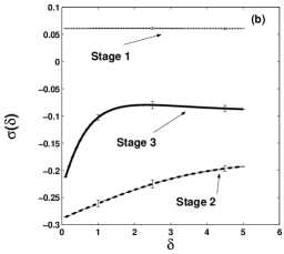
Figure 1: Plots of the measure in time for various moments. $L=32$. (a) The noise-free case for different $\delta$, (b) The slopes versus $\delta$ for Stage 1,2, and 3 for the noise-free case.

The behavior of $\mu(\delta,t)$ is shown in Fig. 1(a). The dynamics can be separated into three stages (marked Stage 1,2, and 3 in the figure). Initially, $\mu(\delta,t)$ appears to grow as a power law in time for about one and a half decades, as seen in Fig. 1(a). There is a formation of small domains from the random initial field. As seen from the topmost curve of Fig. 1(b), the growth rates $\sigma_{1}(\delta,t)$ for all $\delta$ are nearly identical and independent of $t$ . During this stage, one contribution to $\mu(\delta,t)$ comes from points near the domain boundaries. This is seen by plotting the height along any row or column. Although the formation of domains reduces the number of interfacial points , this decrease is countered by the fact that since $\psi(\vec{x},t)$ has not reached its equilibrium values, the internal points of a domain provide an increasing contribution to the integrand. Consequently, $\mu(\delta,t)$ increases during this stage.

The crossover between Stages 1 and 2 occurs when the field $\psi$ saturates to its equilibrium values. A histogram of interfacial heights clearly shows the concentration near the equilibrium values of $\pm 1$. Beyond this stage, interior points of a domain no longer contribute to $\mu(\delta,t)$. As a result, the aforementioned decrease in interfacial boundary points now leads to a decrease in $\mu(\delta,t)$. The slopes $\sigma_{2}(\delta,t)$ in this stage are plotted in the lower curve of Fig. 1(b). We find that in this stage, the distinct moments relax at different rates (i.e, $\sigma_{2}(\delta,t)$ is $\delta$-dependent). Moreover, it is seen from Fig. 1(b) that the rate of relaxation of the larger moments is smaller than that for the lower moments, implying that sharper features (those with larger curvature) change relatively slowly. For example, straightening of a domain boundary wall occurs at a faster rate than elimination of a small domain. Running averages reveal that $\sigma_{2}(\delta,t)$ is uniform until the end of this stage. Observe one critical difference between Stages 1 and 2, namely that the difference in relaxation of the distinct lengthscales cannot be determined without an array of measures.

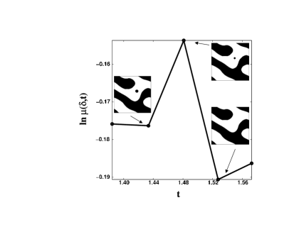
Figure 2: Bubble disappearance for the $L=128$ lattice. The actual time is obtained by scaling the x-axis values by a factor $10^{5}$. Notice how the peak in the measure corresponds to the bubble disappearing at approximately time $148,000$. This is for $\delta=3.4$.

The domain size as measured from the two point correlation function Chakrabarti et al. (1989) becomes comparable to $L$ between Stages 2 and 3 and $\sigma_{2}(\delta,t)$ changes during the transition. The spatio-temporal dynamics beyond this involves a coarsening of the large domains and elimination of the small ones. The disappearance of small domains can be identified by peaks in $\mu(\delta,t)$ for large values of $\delta$. These peaks result from the large curvature of a disappearing domain. Fig. 2 shows the effect of such an event on $\mu(\delta,t)$. It is clear that the elimination of a domain is accompanied by a peak in $\mu(\delta,t)$. The decay rates $\sigma_{3}(\delta,t)$ for the third stage are not uniform in time, unlike the previous stages. An example is shown in the central curve of Fig. 1(b). Although $\sigma_{3}(\delta,t)$ varies in time, the general form is the same; there is a $\delta$-dependence for small values of $\delta$ but a saturation for higher values. At the end of Stage 3, only a handful of large domains remain; the only dynamics beyond this is an extremely slow straightening of the interfaces.

Surface roughness and domain size cannot provide such detailed information on the spatio-temporal dynamics. For a given structure, $W_{L}(t)$ saturates at the end of Stage 1, and there is no discernible difference beyond this. The domain size grows as $R(t)\sim t^{\frac{1}{3}}$ at large times but also saturates between Stage 2 and 3, and gives no further information.

We have also investigated the effect of adding zero-mean external noise to the CHE. We find that in the presence of noise, the dynamics in Stage 3 is faster than in the noise-free case, i.e., $|\sigma_{3}(\delta,t)|$ is larger for the noisy dynamics. We also find that the saturation time of $\mu(\delta,t)$ is proportional to $\sqrt{\epsilon}$.

The KPZ equation is a paradigmatic model of non-equilibrium interfacial growth in the presence of lateral correlations Kardar et al. (1986); Halpin-Healy and Zhang (1995). It gives the local growth of the height profile $h(\vec{x},t)$ at substrate position $\vec{x}$ and time $t$ as

$$\frac{\partial h(x,t)}{\partial t}=\nu{\nabla}^{2}h+{\lambda}{(\nabla h)}^{2}+\eta(\vec{x},t).$$ (3)

Here $\nu$ is the diffusion parameter which smoothens the interface and $\lambda$ the prefactor of the nonlinear term which tends to amplify large slopes. $\eta({\vec{x},t})$ is delta-correlated noise of zero mean which represents a random particle flux. RSOS is a discrete counterpart of the KPZ. Here, particles are added to a randomly chosen site $i$ if and only if the addition ensures that all nearest-neighbor height differences $|\Delta h|\leq\Gamma$, where $\Gamma$ is some pre-determined positive integer.

Roughness and correlation function analyses of the dynamics of both KPZ and RSOS models show that their growth and roughness exponents take similar values in all dimensions, i.e., they are in the same universality class for large values of $\lambda$.

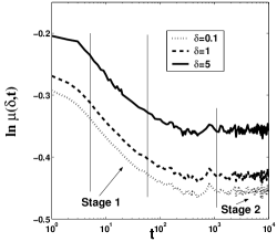
Figure 3: Measure for the KPZ model for different $\delta$. $L=128.$

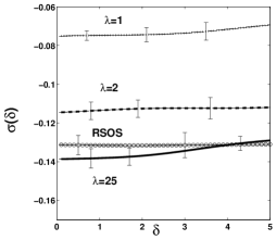
Figure 4: The slopes vs. $\delta$ for various $\lambda$ values compared with the RSOS slopes.

In the initial stages, the correlations spread across the entire lattice and the correlation length $\zeta\sim t^{\frac{1}{z}}$, where $z\sim 1.6$. It has been established numerically Amar and Family (1990) that the strong non-linear coupling limit of KPZ corresponds to the RSOS model in terms of the growth and the saturation exponents of the surface roughness.

The behavior of $\mu(\delta,t)$ in time for the KPZ model ($L=128$) is shown in Fig. 3. The dynamics is qualitatively similar to the behavior of the surface roughness, and can be divided into two distinct stages. In Stage 1, the lateral correlations spread across the entire lattice and we find that $\mu(\delta,t)$ decreases as $t^{-\sigma_{1}(\delta,t)}$ where $\sigma_{1}(\delta,t)$ is independent of $\delta$ and $t$ within numerical errors. The plots labelled by the dotted, dashed and solid lines in Fig. 4 correspond to $\sigma_{1}(\delta,t)$ for three values of $\lambda$ of the KPZ model ($\lambda=1$, $\lambda=2$, and $\lambda=25$ respectively) during the first stage. $\mu(\delta,t)$ for the RSOS model exhibits a similar behavior during Stage 1. In Fig. 4, the plot with circles shows $\sigma_{1}(\delta,t)$ versus $\delta$ for the RSOS model. This corroborates the assertion that for the large $\lambda$ limit, KPZ corresponds to the RSOS models in terms of the growth exponents, since it is seen clearly that $\sigma_{1}(\delta,t)$ for KPZ with $\lambda=25$ and for RSOS are within the errorbars.

In Stage 2 of Fig.3, $\mu(\delta,t)$ saturates to a $L$-dependent value (given by $L^{\gamma(\delta)}$) where $\gamma(\delta)$ is the saturation exponent. However, in this case, we find that $\gamma(\delta)$ for KPZ and RSOS models, even at strong coupling, are very different . For example, $\gamma(\delta)$ for the RSOS model is found to be $\gamma(0.1)=-0.095\pm 0.004$ while that for the KPZ model ($\lambda=25$) is $\gamma(0.1)=-0.075\pm 0.007$ when $\delta=0.1$. For $\delta=1.0$, the saturation exponent for RSOS is $\gamma(1.0)=-0.083\pm 0.002$ while that for the KPZ is $\gamma(1.0)=-0.068\pm 0.007$.

In summary, we have introduced a set of characteristics $\mu(\delta,t)$ that can be used to study spatio-temporal dynamics of systems represented by a scalar field $U(\vec{x},t)$. At a given instant, $\mu(\delta,t)$ are a set of inverse lengthscales associated with a pattern, and are defined in terms of the determinant of the Hessian. Large values of $\delta$ emphasize regions with larger curvature of contour lines.

The availability of a family of indices allows us to provide a more comprehensive description than is possible from individual measures. For example, it was shown for the CHE that during Stage 2, relaxation of the distinct lengthscales associated with the structure occurs at different rates. This is very different from Stage 1 where all such scales grow as $\mu(\delta,t)\sim t^{0.06}$. We are also able to identify instances where small domains of the pattern disappear by searching for peaks in $\mu(\delta,t)$ for large values of $\delta$.

Analysis of the KPZ and the RSOS models shows two stages in pattern evolution. For KPZ, $\mu(\delta,t)$ relaxes at a rate that depends on $\lambda$ during stage 1. The rate of decay $\sigma_{1}(\delta,t)$ for large values of $\lambda$ (typically $\lambda\geq 15$) is seen to be the same as for the RSOS model, thus reinforcing previous claims that both models belong to the same universality class. However, our analysis provides an additional piece of information, namely that all lengthscales $\mu^{-1}(\delta,t)$ associated with the spatio-temporal dynamics of these interfaces decay at the same rate. $\mu(\delta,t)$ saturates in stage 2 for both models, and the saturation value depends on the system size $L$ as $L^{\gamma(\delta)}$. Interestingly, the function $\gamma(\delta)$ for the two models is different; after saturation, the contours of the two models exhibit non-universal characteristics. It is thus possible to determine which of these models better represents the growth of an experimental interface.

The authors thank R. Rajesh and K. E. Bassler for a critical reading of the manuscript and for useful discussions. This research is partially funded by a grant from the National Science Foundation.

References

- Bray (1994) A. J. Bray, Adv. Phys. 43, 357 (1994).
- Kardar et al. (1986) M. Kardar, G. Parisi, and Y.-C. Zhang, Phys. Rev. Lett. 56, 889 (1986).
- Kim and Kosterlitz (1989) J. M. Kim and J. M. Kosterlitz, Phys. Rev. Lett. 62, 2289 (1989).
- Cross and Hohenberg (1993) M. C. Cross and P. C. Hohenberg, Rev. Mod. Phys. 65, 851 (1993).
- Langer (1992) J. S. Langer, Solids Far From Equilibrium, edited by C. Godreche (Cambridge University Press, 1992).
- Family and Vicsek (1991) F. Family and T. Vicsek, Dynamics Of Fractal Surfaces (World Scientific, Singapore, 1991).
- Halpin-Healy and Zhang (1995) T. Halpin-Healy and Y.-C. Zhang, Phys. Rep. 254 (1995).
- Barabasi and Stanley (1995) A.-L. Barabasi and H. E. Stanley, Fractal Concepts In Surface Growth (Cambridge University Press, 1995).
- Sarma and Ghaisas (1992) S. D. Sarma and S. V. Ghaisas, Phys. Rev. Lett. 69, 3762 (1992).
- Sarma et al. (1994) S. D. Sarma, S. V. Ghaisas, and J. M. Kim, Phys. Rev. E 49, 122 (1994).
- Toral et al. (1988) R. Toral, A. Chakrabarti, and J. D. Gunton, Phys. Rev. Lett. 60, 2311 (1988).
- Chakrabarti et al. (1989) A. Chakrabarti, R. Toral, and J. D. Gunton, Phys. Rev. B 39, 4386 (1989).
- Swift and Hohenberg (1977) J. Swift and P. C. Hohenberg, Phys. Rev. A 15, 319 (1977).
- Hu et al. (1995) Y. Hu, R. Ecke, and G. Ahlers, Phys. Rev. E 51, 3263 (1995).
- Gunaratne et al. (1994) G. H. Gunaratne, Q. Ouyang, and H. L. Swinney, Phys. Rev. E 50, 2802 (1994).
- Gunaratne et al. (1995) G. H. Gunaratne, R. E. Jones, Q. Ouyang, and H. L. Swinney, Phys. Rev. Lett. 75, 3281 (1995).
- Gunaratne et al. (1998) G. H. Gunaratne, D. K. Hoffmann, and D. J. Kouri, Phys. Rev. E 57, 5146 (1998).
- Halsey et al. (1986) T. C. Halsey et al., Phys. Rev. A 33, 1141 (1986).
- Hentschel and Procaccia (1983) H. G. E. Hentschel and I. Procaccia, Physica 8D p. 435 (1983).
- Press et al. (1995) W. H. Press, B. P. Flannery, S. A. Teukolsky, and W. T. Vetterling, Numerical Recipes In C (Cambridge University Press, 1995).
- Amar and Family (1990) J. G. Amar and F. Family, Phys. Rev. A 41, 3399 (1990).