A phase-space method for the Bose-Hubbard model

Abstract

We present a phase-space method for the Bose-Hubbard model based on the Q-function representation. In particular, we consider two model Hamiltonians in the mean-field approximation; the first is the standard ”one site” model where quantum tunneling is approximated entirely using mean-field terms; the second ”two site” model explicitly includes tunneling between two adjacent sites while treating tunneling with other neighbouring sites using the mean-field approximation. The ground state is determined by minimizing the classical energy functional subject to quantum mechanical constraints, which take the form of uncertainty relations. For each model Hamiltonian we compare the ground state results from the Q-function method with the exact numerical solution. The results from the Q-function method, which are easy to compute, give a good qualitative description of the main features of the Bose-Hubbard model including the superfluid to Mott insulator. We find the quantum mechanical constraints dominate the problem and show there are some limitations of the method particularly in the weak lattice regime.

1 Introduction

The prediction [1] that a Bose-Hubbard Hamiltonian could be realized with cold Bosonic atoms trapped in an optical lattice, and the transition between superfluid and Mott-insulator phases observed, led to the development of an experiment in which these predictions were verified [2], and has lent urgency to the quest for a computationally simple description of the phenomena involved. It is desirable to find a description which can cover both of the two regimes of qualitatively different behaviour:

• Weak Lattice, when the atoms are delocalized, and are thus highly mobile; the system is weakly correlated.

• Strong Lattice, when the atoms are localized; the system is highly correlated. In this case there are two subcases

  • Commensurate, when the number of atoms per site is integral, and the state is a product of number states on each site. In this case there can be no mean-field.

  • Incommensurate, when the number of atoms per site is non-integral, and in this case there can be a mean-field.

In the case of an integral average site filling, as the strength of the lattice varies, a transition from the delocalized to the localized situation takes place, and one passes from state with a non-zero mean-field to a state with no mean-field. Conventionally, if there is no mean-field, one speaks of a Mott insulator phase, while if there is a non-vanishing mean-field, the terminology superfluid phase is applied.

The dynamics of the Bose-Hubbard model in states for the strong lattice region presents formidable technical difficulties. The so-called Gutzwiller approximation [1] has been used in several treatments, but because it represents the wavefunction as a product of wavefunctions at different sites, the description of intersite correlations is necessarily very approximate. Progress has been made [3, 4] in regions near to the weak lattice regime by using a self-consistent Bogoliubov method, in which the statistics of the quantum fluctuations are treated by what amounts to a Gaussian ansatz. However, this method cannot be used near the strong lattice regime because in this case the statistics are far from Gaussian.

1.1 Overview

In this paper we want to introduce approximate methods which should be applicable in both the superfluid and the Mott insulator regimes, and to show their efficacy in the very simplest method used for the Bose-Hubbard model, that of static mean-field theory. We propose a phase space method from quantum optics based on the Q-function representation which involves an approximate reparamterization of the Bose-Hubbard Hamiltonian in terms of Gaussian variables. The advantage of this methodology lies in the simple description of a wide range of quantum states for the system.

We apply this method to two approximations to the Bose-Hubbard Hamiltonian which we denote as the one site and two site models. The one site model treats all intersite correlations (ie. tunnelling to adjacent sites) by a mean-field term, which essentially decouples the total Hamiltonian into a sum of one site Hamiltonians. This has already been introduced with the Hamiltonian given by (2). The two site model extends this formulation by explicitly including intersite correlations between two adjacent sites, while treating the interactions with neighbouring sites using the mean-field approximation.

For the one site Q-function approach, we find rather good agreement over all regimes, with the advantage that our phase space method can be evaluated very easily—in a matter of seconds on any reasonable workstation. The accuracy is usually about 5%, with the qualitative behavior being accurately given. The essence of the result is that the ground state is essentially that wavefunction which minimizes the classical energy functional subject to the inequality constraints given by the uncertainty principle in two different forms.

These results are compared with an exact numerical solution to the one site model using arbitrary one site states. In this case, the solution is found by reparameterizing the energy in terms of the number variance and finding the maximum mean-field for which the energy is minimized. The formulation is equivalent to the application of the standard Gutzwiller ansatz.

The Q-function formulation is easily extended to the two site model when lattice homogeniety is assumed. The correct description of the two site quantum statistics requires the inclusion of additional constraints which are used to determine the ground state solution. The results here give a good qualitative description of the overall features of the Bose-Hubbard model. However, a shortcoming of the parameterization on two sites is highlighted by the failure of the method to correctly predict the Mott insulator phase, as determined by a vanishing mean-field, when compared to the results from sections 3, 4 and 6.

The two site model is also solved by exact numerical minimization with the assumption of lattice symmetry giving a reduced Hilbert space. Here, the ground state results show the pertinent features of the Bose-Hubbard model, with a vanishing mean-field throughout the Mott insulator phase, which is an improvement over the two site Q-function formulation. The results are compared with other reports from the literature, including density matrix renormalization group and Quantum Monte-Carlo methods, which yield numerically exact results for one dimensional finite lattices.

2 Bose-Hubbard Hamiltonian

In order to set our notation and define terminology, we will summarize the basics of the Bose-Hubbard model—first introduced by Fisher et al. [5] to describe the superfluid-insulator transition in liquid ⁴He, but applicable more generally to any system with interacting bosons on a lattice. The simplest form of the model is given when the atoms are loaded adiabatically into the lattice, so that they remain in the lowest vibrational state. As we will be formulating the model using the Q-function representation, and noting that this distribution is adapted to antinormal ordering, we write the Bose-Hubbard Hamiltonian in the antinormally ordered form

$$H = -\sum_{i,j}t_{ij}a_{i}a^{\dagger}_{j}+u\sum_{i}a_{i}a_{i}a_{i}^{\dagger}a_{i}^{\dagger}.$$ (1)

where $a_{i}^{\dagger}$ and $a_{i}$ respectively are the creation and annihilation operators for a boson on the $i$th lattice site. The first term of the Hamiltonian describes the quantum tunelling (hopping) between neighboring sites with an amplitude $t_{ij}$ which is only non-zero when $i$ and $j$ are adjacent. The second term represents the on-site interaction energy which is taken as repulsive with $u\geq 0$. We note that this Hamiltonian is easily related to its normally ordered counterpart using the commutation relation $[a_{i},a_{j}^{\dagger}]=\delta_{ij}$.

2.1 The mean-field approximation

In the mean-field approximation, one assumes that the effect of the the nearest neighbours on the site $i$ is given by a c-number mean-field ${\cal E}=\langle a_{i}\rangle$ which, by a choice of phase, we take as real, and which is independent of $i$ for a homogeneous system. Thus we can write

$$H \to H_{\rm mf}=\sum_{i}\left\{-{Z\over 2}{\cal E}(a^{\dagger}_{i}+a_{i})+ua_{i}a_{i}a_{i}^{\dagger}a_{i}^{\dagger}\right\}$$ (2)

where $Z$ is proportional to the nearest neighbor value of $t_{ij}$ multiplied by the number of nearest neighbours. As noted in Sachdev’s book [6], to solve the system one finds the lowest eigenvalue of $H_{\rm mf}$ on a single site, for which the value of ${\cal E}$ must match that of $\langle a_{i}\rangle$.

         

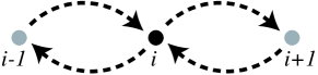
(a) One site model

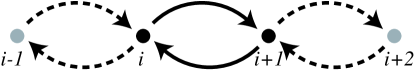
(b) Two site model

Figure 1: Treatment of hopping terms in the Bose-Hubbard model for a lattice of dimension $d=1$. The dashed arrows indicate those hopping terms $t_{ij}a_{i}a_{j}^{\dagger}$ included by a mean-field approximation, whereas the solid arrows indicate those terms included explicitly in the Hamiltonian. We consider two formulations: (a) The hopping terms between the $i$th site and it’s $z=2d$ nearest neighbours are treated solely by a mean-field approximation; (b) The hopping terms between two adjacent sites $i$ and $i\!+\!1$ are included explicitly, whereas the hopping terms between each of these sites and and their (other) nearest $z^{\prime}=2d-1$ neighbours are included using the mean-field approximation.

Thus, one assumes a value for the mean-field, computes the ground state eigenfunctions of the Hamiltonian, whose mean-field should equal that initially assumed. Unlike the more conventional method, we do this at fixed mean occupation of the site, not fixed chemical potential, and compute the chemical potential from the energy. Since the solutions of this process are well known, it will provide an interesting testbed for the phase space method we wish to propose.

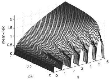
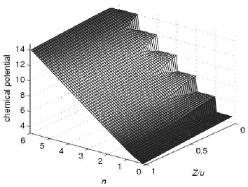
Figure 2: Ground state phase diagram for the Bose-Hubbard model using a self-consistent mean-field approach; the mean-field and chemical potential are both shown as a function of the relative interaction strength $Z/u$ and mean occupation number $n$ (normal ordered).

2.2 Self-consistent mean-field results

The results obtained by this procedure are shown in Fig.2. The usual features of the superfluid to Mott insulator transition are present. In particular, in the Mott insulator phase, the mean-field vanishes for commensurate occupations when the relative interaction strength ($Z/u$) is below a critical value. There is a corresponding energy gap evident in the chemical potential which represents the energy required to add or remove a particle to the system; hence the Mott phase is incompressible. When the density is incommensurate or the tunnelling dominates, there is a transition to the superfluid phase where the mean-field is non-zero.

PART I: ONE SITE FORMULATION

3 Q-functions for one site states

We first introduce the Q-function parameterization and its application to the one site Hamiltonian (2) for the Bose-Hubbard model.

3.1 Phase space methods

The field of quantum optics leads to various quasi-classical distributions [7] which can be used to treat quantum processes using a c-number formalism in terms of coherent states $|\alpha\rangle$. For a one-mode system with density operator $\rho$, the most widely used of these are given by

• The Q-function:

  $$Q(\alpha,\alpha^{*}) = \langle\alpha|\rho|\alpha\rangle/\pi.$$ (3)

  The Q-function is a quasiprobablity for antinormally ordered operator averages, that is

  $$\langle a^{n}(a^{\dagger})^{m}\rangle = \int d^{2}\alpha\,\alpha^{n}({\alpha^{*}})^{m}Q(\alpha,\alpha^{*})$$ (4)

  It always exists and is positive

• The P-function: $P(\alpha,\alpha^{*})$ with $\rho=\int d^{2}\alpha P(\alpha,\alpha^{*})|\alpha\rangle\langle\alpha|$, associated with normally ordered moments. However, it does not always exist as a positive well behaved function.

• The Wigner function: $W(\alpha,\alpha^{*})$, is associated with symmetric operator ordering, and always exists, but is not always positive.

• The positive P-function: $P(\alpha,\beta)$, a P-function defined in a doubled phase-space, always exists and is positive, but does present some technical difficulties [7].

We develop a treatment in terms of the Q-function, since this is always positive and well-defined, and is thus a genuine probability density to which we can apply probabilistic approximations. It can be used to describe a wide range of states for the Bose-Hubbard model which interpolate between the extremes:

• Weak lattice: in the case that the hopping dominates ($t_{ij}$ very large) the ground state is the product of coherent states at each site.

• Strong lattice: in the other extreme, when the hopping is negligible, the ground state is the product of eigenstates at each site. If the mean occupation per site is $n$ and $[n]$ denotes the integer part of $n$, then the state at each site is a superposition of number states of the form $\sqrt{\lambda}|[n]\rangle+\sqrt{1-\lambda}|[n]+1\rangle$, where $\lambda$ is chosen to give the correct mean occupation. These states are not Gaussian.

The Gaussian or non-Gaussian nature of the statistics in the Bose-Hubbard model is very important, and one of the virtues of the Q-function is that it is Gaussian when the quantum statistics is also Gaussian [7].

The Q-functions for the three principal kinds of states are:

• Number state: The Q-function for a number state is

  $$Q_{n}(\alpha,\alpha^{*}) = {1\over\pi}{e^{-|\alpha|^{2}}|\alpha|^{2n}\over n!}.$$ (5)

  Examples of this distribution appear in Fig.3 (a) and (e). The distribution has a characteristic ring shape, which is clearly non-Gaussian.

• Superposition of number states The Q-function for the superposition of number states with $n-1$ and $n$ atoms in proportions $1-\lambda:\lambda$ is

  $$Q_{{\rm sup}\lambda}(\alpha,\alpha^{*}) = {1\over\pi}\left|\sqrt{1-\lambda}+\alpha\sqrt{\lambda\over n}\right|^{2}{e^{-|\alpha|^{2}}|\alpha|^{2(n-1)}\over(n-1)!}.$$

  This is the kind of state expected with an incommensurate filling in the limit of no hopping. The Q-function then varies between a ring shaped distribution for $\lambda=0,1$ to a rather distorted Gaussian distribution at $\lambda=1/2$; see Fig.3 (a)–(e).

• Coherent state In the superfluid case with mean filling per site $n$, where the hopping is dominant, we expect an approximately coherent state with parameter $\beta=\exp(i\theta)\sqrt{n}$, for some real $\theta$, and then the Q-function has the Gaussian form

  $$Q_{{\rm coh},\beta} = {1\over\pi}\exp\left(-|\alpha-\beta|^{2}\right).$$ (7)

  This is plotted in Fig.3 (f).

.

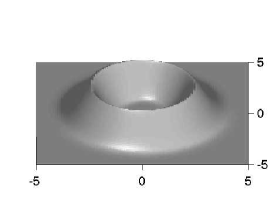
(a) $n=7$, $\lambda=0$

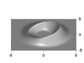
(b) $n=7$, $\lambda=0.15$

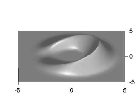
(c) $n=7$, $\lambda=0.5$

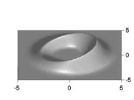
(d) $n=7$, $\lambda=0.85$

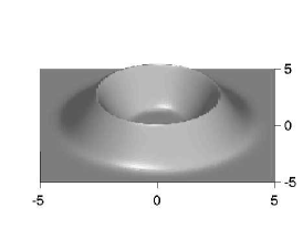
(e) $n=7$, $\lambda=1$

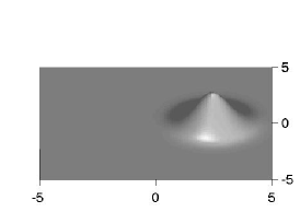
(f) coherent state, $\beta=\sqrt{6}$, $\lambda=0$

Figure 3: Q-function for the superposition of $n=6$ and $n=7$ states in proportion 1:0, 0.85:0.15, 0.5:0.5, 0.15:0.85, 0:1; and for a coherent state with $\beta=\sqrt{6}$

3.2 Parametrization of the Q-function

The probability distributions of Fig.3 can be approximately parametrized by writing the random variable ${a}\to\alpha$ with

$$\alpha = (v+\delta)e^{i\theta}$$ (8)

where

• $v$ is a nonrandom positive real quantity;

• $\delta$ is a Gaussian random variable with zero mean and variance $\sigma$;

• $\theta$ is a Gaussian random variable with a mean which is in principle nonzero, but which by choice of phase definition can be chosen to be zero, and with variance $\Delta$. In this case, the averages of powers of $\exp(i\theta)$ are given by

  $$\langle e^{pi\theta}\rangle=\exp\left({-p^{2}\Delta/2}\right)\equiv c^{p^{2}}.$$ (9)

Using properties of Gaussian variables this approximation leads to the values of the antinormally ordered moments:

$$\langle{a}\rangle = vc$$ (10)

$$\langle{a}{a}^{\dagger}\rangle = (v^{2}+\sigma)$$ (11)

$$\langle{a}{a}\rangle = (v^{2}+\sigma)c^{4}$$ (12)

$$\langle{a}{a}{a}^{\dagger}\rangle = (v^{3}+3\sigma v)c$$ (13)

$$\langle{a}{a}{a}^{\dagger}{a}^{\dagger}\rangle = (v^{4}+6v^{2}\sigma+3\sigma^{2})$$ (14)

Note that the first of these moments (10) represents the mean-field. A straightforward extension of this this parameterization to $L$ sites can be given by the substitution $a_{k}\rightarrow(v_{k}+\delta_{k})e^{i\theta_{k}}$ for $k=1,2,...,L$; we make use of this for the two site problem presented in section 5.

Validity of parameterization: values of the parameters in particular cases

To fit the kinds of distribution in Fig.3 we determine the parameters $v$, $\sigma$ and $c$ by fitting the moments $\langle{a}\rangle$, $\langle{a}{a}^{\dagger}\rangle$ and $\langle{a}{a}{a}^{\dagger}{a}^{\dagger}\rangle$. These are given in detail in A, where we show that for a wide variety of states we get very tolerable approximations. Thus we can expect a good qualitative description of the system for an arbitrary lattice strength. However, we note that the parameterization is least accurate in the case of an equal superposition of number states which we will find reflected in the ground state phase diagram in the strong lattice regime.

3.3 Determination of the ground state

Using the Hamiltonian (2) and the moments (10)–(14), the average energy in the Q-function representation is

$$E(n,c,v) = -Zc^{2}v^{2}+u(3n^{2}-2v^{4}).$$ (15)

To find the ground state solution at a given interaction strength $Z/u$ and mean occupation $n$, this quantity is minimized with respect to the free parameters $v$ and $c$, with the bounds $v\geq 0$ and $0\leq c\leq 1$ as permitted by the Q-function parameterization.

3.3.1 Constraints

The functional (15) is a classical distribution that has no local minima so that the minimum must occur on the boundary. However the system should be governed by the quantum mechanical nature of the problem, which we reintroduce in the form of two constraints on the minimization procedure, one derived from a restriction on the number variance, the other from the uncertainty relation for the conjugate variables of phase and number.

The most significant of the constraints enforced by the quantum mechanical nature of the problem are as follows.

Fractionality constraint

If the mean occupation per site is non-integral, the variance of the occupation must be nonzero, and this has a major bearing on the problem, which we shall formulate precisely. We will be considering cases where the mean occupation per site is fixed, so that

$$\langle{a}{a}^{\dagger}\rangle = n\geq 1$$ (16)

so that

$$n = v^{2}+\sigma\geq 1.$$ (17)

Setting

$$N = {a}{a}^{\dagger}$$ (18)

and using (10)-(14) the variance of the site occupations is

$${\rm var}[N] \equiv \langle{a}{a}^{\dagger}{a}{a}^{\dagger}\rangle-\langle{a}{a}^{\dagger}\rangle^{2}$$ (19)

$$= 2n^{2}-n-2v^{4}.$$

In $n$ is non-integral, with fractional part $\delta n$, then the minimum variance for a given $n$ occurs when only the two occupation numbers which bracket the value $n$ are represented, and then this gives a variance of $\delta n(1-\delta n)$, leading to the constraint

$${\rm var}[N] \geq \delta n(1-\delta n).$$ (20)

and using (19) we can write this as

$$0 \leq v^{4}\leq n^{2}-{1\over 2}\bigg{(}n+\delta n(1-\delta n)\bigg{)}$$ (21)

Phase-number uncertainty relations

The uncertainty principle enters when we consider that phase and number are conjugate variables. We can write a rigorous uncertainty relationship using

$$X={{a}+{a}^{\dagger}\over 2};\qquad Y={{a}-{a}^{\dagger}\over 2i}$$ (22)

so that we have the commutation relations

$$[N,X] = -iY;\qquad[N,Y]=iX$$ (23)

from which follow an uncertainty relation

$$\langle\delta Y^{2}\rangle{\rm var}[N] \geq {1\over 4}\langle X\rangle^{2}$$ (24)

In our formulation we have chosen a zero mean phase so that $\langle Y\rangle=0$ (see (128)) and thus $\langle\delta Y^{2}\rangle=\langle Y^{2}\rangle$. Using (128–132), and antinormally ordering all the products involved, we find

$$\langle\delta Y^{2}\rangle = {n\over 2}(1-c^{4})-{1\over 4}$$ (25)

and thus

$$\left[{n\over 2}(1-c^{4})-{1\over 4}\right]\left(2n^{2}-{n}-2v^{4}\right) \geq {1\over 4}v^{2}c^{2}.$$ (26)

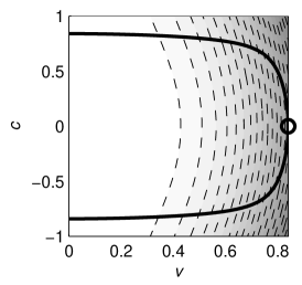
(a) $n=1$, $Z/u=0.5$

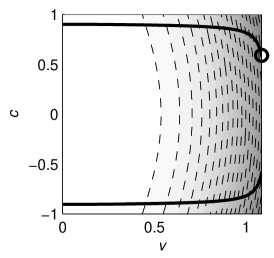
(b) $n=1.5$, $Z/u=0.5$

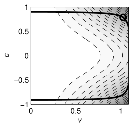
(c) $n=1.5$, $Z/u=10$

Figure 4: Level curves of energy (15) in the Q-function representation for three different cases are indicated by the dashed curves, with the energy decreasing for darker regions; the permissable parameter space for $v$ and $c$ is given by the bounds $v\geq 0$ and $0\leq|c|\leq 1$ (for purely illustrative purposes we allow $c$ to be negative here because the problem is symmetrical about $c=0$) where $v$ is further bounded by (21). Since (15) has no local minima, the minimum energy occurs within the shown bounded region and subject to the constraint (26) derived from the phase-number uncertainty relation which is shown by the solid curve. The solution in each case is indicated by a circle. In the first case ($n=1$, $Z/u=0.5$) this occurs for $c=0$ so that the mean-field is zero; in the second case ($n=1.5$, $Z/u=0.5$) this occurs for a non-zero $c$ so that there is a mean-field. In both these cases, the solution saturates the upper bound for $v$. Conversely, in the third case ($n=1.5$, $Z/u=10$) where the lattice is weak, the solution occurs within the bounded region.

3.3.2 Results

Minimizing (15) with the constraints (21) and (26) leads to the ground state phase diagram shown in Fig.5. These results compare well with the exact solution shown in Fig.2, particularly with confirmation of the Mott insulator phase at commensurate occupations for a strong lattice (small $Z/u$), and of the superfluid phase for a weak lattice (large $Z/u$).

The results are dominated by the interplay between the constraints, which is made evident by considering Fig.4. In the strong lattice regime, the ground state solution is given at the intersection of the fractionality constraint (21) which determines the upper bound for $v$, and the phase-number uncertainty constraint (26), shown by the solid curve. Specifically for $Z/u=0.5$, and for an integer $n=1$, this occurs at $c=0$ and the resulting vanishing mean-field is indicative of the Mott insulator phase; for a non-integer $n=1.5$ the solution occurs for $c\neq 0$ so that there is a non-zero mean-field corresponding to a superfluid component. Conversely for a weak lattice, with $n=1.5$ and $Z/u=10$, the solution is determined solely by(26).

The fact that the quantum mechanical constraints dominate the problem is not unexpected as the phase transition between the Mott insulator and superfluid is driven by quantum fluctuations.

We note that for the Q-function results at half-integer values of $n$, the mean-field remains constant over some range of $Z/u$ in the strong lattice regime. This contrasts with the numerically exact results obtained by a self-consistent mean-field approach as shown in Fig.2 where the mean-field is a monotonically increasing function of $Z/u$. This difference arises from the weaker approximation of the Q-function parameterization in the case of an equal superposition of number states as shown in Fig.3 (c), and quantified in A.

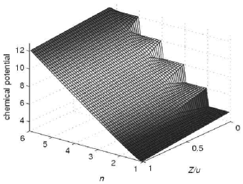
Figure 5: Ground state results for Bose-Hubbard model with Q-function representation; the mean-field and chemical potential are shown as a function of relative interaction strength $Z/u$ and (anti-normal ordered) occupation $n$.

4 Exact numerical minimization of one site problem

The inequalities (26) and (21) restrict the mean-field to a certain maximum value, but this maximum may not be optimal. Let us then pose the question: What is the largest value of the mean-field for a given mean number and variance. This value determines the minimum energy and permits the following basic strategy for finding the ground state phase diagram. Firstly, reparameterize the mean-field in terms of the mean number occupation and number variance; and secondly, minimize the energy with respect to the number variance at a fixed relative interaction strength $zt/u$ and mean occupation. The problem is then essentially reduced to a minimization of energy with respect to a single variable – the number variance.

4.1 Formulation using one site states

Here we give an exact numerical procedure for determining the ground state of the Bose-Hubbard model in the one site mean-field approximation. A one site quantum state can be written as a superposition of number states

$$|s\rangle=\sum_{n}c_{n}|n\rangle$$ (27)

where the usual normalisation condition ($1=\langle s|s\rangle$) applies. In this basis the mean-field is

$$\langle X\rangle=\langle s|\frac{a+a^{\dagger}}{2}|s\rangle=\Re\left\{\sum\sqrt{n}\,c^{*}_{n-1}c_{n}\right\}$$ (28)

The Hamiltonian (2) leads to the expression for the one site energy in the mean-field approximation

$$\langle E\rangle=-Z\,{\langle X\rangle}^{2}+u\big{(}2+{\rm var}[N]+\overline{n}^{2}+3\,\overline{n}\big{)}$$ (29)

where $\overline{n}\equiv\langle a^{\dagger}\,a\rangle$ is the (normal ordered) mean number and ${\rm var}[N]=\overline{n^{2}}-\overline{n}^{2}$ is the number variance of atoms on each site (note the normal and anti-normal ordered means are related by $\langle a^{\dagger}a\rangle=\langle aa^{\dagger}\rangle-1$). Since the chemical potential term has been omitted in (1), we treat the system using the canonical ensemble by taking a fixed number of atoms in the lattice, that is by explicitly using the constraint of fixed mean occupation.

Clearly, the energy functional (29) is then minimised when the mean-field $\langle X\rangle$ is a maximum and subject to the constraints of normalisation and fixed number mean and variance. In terms of the one site state (27) these constraints are given by

$$\phi_{1}=\sum_{n}|c_{n}|^{2}-1=0\textrm{ (normalization)}$$ (30)

$$\phi_{2}=\sum_{n}|c_{n}|^{2}\,n-\overline{n}=0\textrm{ (fixed mean)}$$ (31)

$$\phi_{3}=\sum_{n}|c_{n}|^{2}\,n^{2}-\overline{n^{2}}=0\textrm{ (fixed variance)}$$ (32)

Moreover, since the constraints are independent of phase, the mean-field (28) is maximized by choosing the set of $c_{n}$ to be real and positive at fixed $|c_{n}|$. To deal with the problem of constrained optimisation we apply the method of Lagrange multipliers; the mean-field is maximized when

$$0=\frac{\partial\langle X\rangle}{\partial c_{n}}-\frac{1}{2}\lambda\,\frac{\partial\phi_{1}}{\partial c_{n}}+\frac{1}{2}\mu\,\frac{\partial\phi_{2}}{\partial c_{n}}+\frac{1}{2}\nu\,\frac{\partial\phi_{3}}{\partial c_{n}}$$ (33)

Note the scalar factors that appear before the Lagrange multipliers ($\lambda$, $\mu$ and $\nu$) are included for convenience. Equation (33) along with equations (28) and (30)–(32) then lead to

$$\sqrt{n}\,c_{n-1}+\sqrt{n\!+\!1}\,c_{n+1}+(\mu\,n+\nu\,n^{2})\,c_{n}=\lambda\,c_{n}$$ (34)

This is a Hermitian eigenvalue problem which has only one eigenvector solution with the set $c_{n}$ all positive, since the solutions form an orthonormal basis (solutions with some $c_{n}$ vanishing may cause ambiguities in principle however).

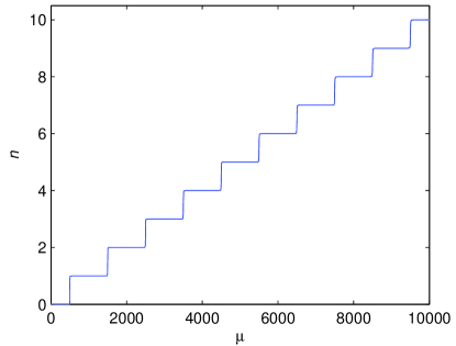
Figure 6: Mean number occupation as a function of $\mu$ at $\nu=-500$ for the one site model. The Lagrange multiplier $\mu$ plays the role of (but is not equal to) the chemical potential; the horizontal regions are indicative of the system near the incompressible Mott insulator phase where $\partial\overline{n}/\partial\mu=0$.

4.2 Numerical Solutions

Numerical solutions of (34) determine the maximum mean-field in terms of ${\rm var}[N]$ and $\overline{n}$. By choosing a fixed $Z/u$ and $\overline{n}$ the calculation of the ground state energy then amounts to a direct minimization of (29) with respect to the variance ${\rm var}[N]$.

We outline the procedure as follows. First, for an appropriate range of the Lagrange multipliers $(\mu,\,\nu)$ the eigenvector solutions of (34) are used to calculate corresponding values of $\overline{n}$, ${\rm var}[N]$ and the maximum mean-field $\langle X\rangle$. A fixed value of $\nu$ determines a $\overline{n}(\mu)$ curve (see for example Fig.6) which is inverted using linear interpolation - with an additional optimization step - to give $\mu$ on a uniform set of $\overline{n}$ points. That is, each value of $\overline{n}$ determines a curve in $\mu$ and $\nu$ from which the dependence of $\langle X\rangle$ on ${\rm var}[N]$ is determined from solutions to (34). Since this relationship is determined on a finite set of points, it is necessary in practice to use cubic interpolation to determine $\langle X\rangle$ for arbitrary ${\rm var}[N]$.

Calculations of $\langle X\rangle$ as a function of ${\rm var}[N]$ are shown in Fig.7 for commensurate and incommensurate mean site occupations; the corresponding curves which arise from the uncertainty relation (26) are shown to be very similar. Note that for commensurate mean occupations the mean-field and variance simultaneously approach zero, corresponding to the Mott insulator phase (a pure number state). In contrast, in the incommensurate case neither the mean-field nor variance approach zero; even in the strong lattice regime there is a non-zero superfluid component, corresponding to a superposition of two number states. Using these curves, the energy (29) can be minimized with respect to ${\rm var}[N]$. This leads to ground state results that are the same numerically as those of the self-consistent mean-field approach shown in Fig.2.

Although the difference in the two sets of curves shown in Fig.7 appears slight, it is entirely responsible for the notable difference between the exact one site calculation (Fig.2) and the approximate phase-space calculation (Fig.5). In the incommensurate case, the fact that the exact curves drop rapidly as ${\rm var}[N]\rightarrow 1/4$ is responsible for the sloping behaviour of the mean-field arches shown in Fig.2 as opposed to the level behaviour shown in Fig.5.

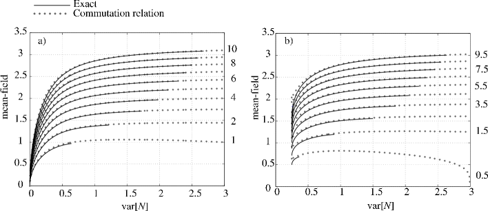
Figure 7: Mean-field versus variance for commensurate (a) and incommensurate (b) mean site occupations for the one site case.

Numerical calculations were performed using the MATLAB software package. The state space was truncated with $n\leq 40$ as this provided a good trade-off between computational efficiency and accuracy (ie. this truncation introduced negligible error to solutions in the region of interest $\overline{n}\leq 10$). Note, to cover a sufficient $\overline{n}$ and ${\rm var}[N]$ range, $(\mu,\nu)$ were chosen from the triangular region with $-800\leq\nu\leq-0.01$ and $0\leq\mu\leq-40\,\nu$. The minimization procedure used the MATLAB fminbnd (bounded minimization) function, with a lower bound for the number variance determined by the fractionality constraint (20).

4.3 Calculating the phase transition boundary

To check the validity of the one site formulation near the transition point, it is useful to calculate the the position of the phase boundary between the superfluid and Mott insulator phases. This can be done approximately by a perturbation method where the ground state energy is determined by states near the transition point. We consider a normalised state of commensurate occupation $\overline{n}$ near the transition point

$$|s\rangle=\sqrt{1-2\lambda}\,|\overline{n}\rangle+\sqrt{\lambda}\,(e^{i\theta_{1}}|\overline{n}-1\rangle+e^{i\theta_{2}}|\overline{n}+1\rangle)$$ (35)

where $\lambda$ is a real and small; $\lambda=0$ corresponds to the Mott insulating phase with a commensurate occupation $\overline{n}$. States with $\lambda\geq 0$ characterize the superfluid phase where the mean-field is non-zero. The corresponding one site energy (29) is given by

$$\overline{E} = -\lambda(1-2\lambda)\,(\sqrt{\overline{n}}\cos{\theta_{1}}+\sqrt{\overline{n}+1}\cos{\theta_{2}})^{2}$$ (36)

$$+\overline{u}(2+2\lambda+\overline{n}^{2}+3\overline{n})$$

Note that in scaling by the factor $1/zt$ this form of the energy is dimensionless and we have defined the ratio $\overline{u}\equiv u/zt$ for the relative interaction strength. The ground state is determined by the minimum energy with respect to variations in the free parameters: $\lambda$, $\theta_{1}$ and $\theta_{2}$. Clearly this occurs for $\theta_{1}=\theta_{2}=0$ (the result $\theta_{1}=\theta_{2}=\pi$ gives the same ground state energy and is equivalent to a change in the sign of the mean-field) and when

$$\frac{\partial{\overline{E}}}{\partial{\lambda}}=0=-(1-4\lambda)(\sqrt{\overline{n}}\cos{\theta_{1}}+\sqrt{\overline{n}+1}\cos{\theta_{2}})^{2}+2\overline{u}$$ (37)

The transition to a Mott insulator phase occurs in the limit $\lambda\rightarrow 0$ when the mean-field goes to zero. Applying this condition, the critial point for the transition is then given by

$$\overline{u}_{c}=\textstyle\frac{1}{2}(\sqrt{\overline{n}}+\sqrt{\overline{n}+1})^{2}$$ (38)

For values of the relative interaction strength above the critical value $\overline{u}>\overline{u}_{c}$ the ground state solution saturates the bound at $\lambda=0$ and the system remains in the Mott insulator phase.

Comparison to other work

In order to compare our results with those reported elsewhere we define the parameter

$$\overline{U}_{c}\equiv 2(u/zt)_{c}$$ (39)

to describe the relative interaction strength at the critical point. The factor of 2 is included because the on-site interaction term $u$ in the Hamiltonian (1) is equivalent to the term $U/2$ which has been used elsewhere (see [4] and [8] for example).

Equation (38) then becomes $\overline{U}_{c}=(\sqrt{\overline{n}}+\sqrt{\overline{n}+1})^{2}$, an expression also found elsewhere [4, 9]; this yields the following values for the transition: $\overline{U}_{c}=5.83$ for $\overline{n}=1$, $\overline{U}_{c}=9.90$ for $\overline{n}=2$, $\overline{U}_{c}=13.93$ for $\overline{n}=3$.

PART II: TWO SITE FORMULATION

The one site formulation necessarily neglects correlations between neighbouring sites in the mean-field approximation. We can improve on this by using a Hamiltonian that explicity includes hopping between two adjacent sites while still treating interactions with other neighbouring sites with the mean-field approximation. In particular consider two adjacent sites labelled by $1$ and $2$ corresponding to sites $i$ and $i+1$ respectively as shown in Fig. 1(b). Following the one site case (1) we can write the Bose-Hubbard Hamiltonian in a two site mean-field approximation as

$$H_{\mbox{\scriptsize two site}}= -t\left[a_{1}a_{2}^{\dagger}+a_{2}a_{1}^{\dagger}+(2d\!-\!1)\left(\textstyle\frac{1}{2}{\cal E}(a_{1}+a_{1}^{\dagger})+\textstyle\frac{1}{2}{\cal E}(a_{2}+a_{2}^{\dagger})\right)\right]$$ (40)

$$+u\,(a_{1}a_{1}a_{1}^{\dagger}a_{1}^{\dagger}+a_{2}a_{2}a_{2}^{\dagger}a_{2}^{\dagger})$$

for a homogenous lattice of dimension $d$ where ${\cal E}=\langle a_{k}\rangle$ (for $k\neq 1,\,2$) is the mean-field representing the interaction with nearest neighbours, which as with the one site model, by a choice of phase is taken as real.

5 Q-function parameterization on two sites

In this case the Q-function parameterization becomes

$$a_{1}\rightarrow\alpha_{1}=(v_{1}+\delta_{1})e^{i\theta_{1}}$$ (41)

$$a_{2}\rightarrow\alpha_{2}=(v_{2}+\delta_{2})e^{i\theta_{2}}$$ (42)

We define the intersite correlation operators

$$b\equiv a_{1}a_{2}^{\dagger};\qquad b^{\dagger}\equiv a_{2}a_{1}^{\dagger}$$ (43)

The corresponding moments are

$$\langle b\rangle=\langle b^{\dagger}\rangle=(v_{1}v_{2}+w)g$$ (44)

where we have set

$$w\equiv\langle\delta_{1}\delta_{2}\rangle$$ (45)

$$g\equiv\langle e^{i(\theta_{1}-\theta_{2})}\rangle$$ (46)

and assumed that the phase and number correlations are independent; although this assumption is possibly not strictly valid, without it the formalism becomes significantly more complicated.

The two site Hamiltonian (40) leads to the expression for the average energy

$$E = \langle H_{\mbox{\scriptsize two site}}\rangle$$ (47)

$$= -\overline{t}\left[2(v_{1}v_{2}+w)g+(2d-1)(v_{1}^{2}c_{1}^{2}+v_{2}^{2}c_{2}^{2})\right]$$

$$+3n_{1}^{2}-2v_{1}^{4}+3n_{2}^{2}-2v_{2}^{4}$$

which has been normalised by dividing through by $u$ and defining the relative interaction strength $\overline{t}\equiv t/u$.

5.1 Constraints

Following the one site case, to find the ground state solution, the energy (47) is minimized subject to constraints arising from any applicable uncertainty relations. In particular, in addition to the constraints (21) and (26) that have already been introduced for the one site statistics, we can derive further constraints that account for the two site statistics by considering commutation relations between bilinear operators.

Variances and covariance

In deriving the necessary constraints for the two site problem, we first consider the following operators

$$N\equiv\frac{N_{1}+N_{2}}{2}$$ (48)

$$M\equiv\frac{N_{1}-N_{2}}{2}$$ (49)

The corresponding variances for each of these operators are given by

$$\textrm{var}[N]=1/4(\textrm{var}[N_{1}]+\textrm{var}[N_{2}]+2\,\textrm{cov}(N_{1},N_{2}))$$ (50)

$$\textrm{var}[M]=1/4(\textrm{var}[N_{1}]+\textrm{var}[N_{2}]-2\,\textrm{cov}(N_{1},N_{2}))$$ (51)

where the number covariance function is given by

$$\textrm{cov}(N_{1},N_{2}) \equiv \langle N_{1}N_{2}\rangle-\langle N_{1}\rangle\langle N_{2}\rangle$$ (52)

$$= 2(2v_{1}v_{2}w+w^{2})$$

with the one site variances, $\textrm{var}[N_{1}]$ and $\textrm{var}[N_{2}]$, given analogously to (19).

Commutation relations

We define the following operators

$$V\equiv\frac{b+b^{\dagger}}{2}$$ (53)

$$W\equiv\frac{b-b^{\dagger}}{2i}$$ (54)

$\langle V\rangle$ is the intersite correlation and gives a measure of particle exchange, or tunnelling, between adjacent sites. Eqs. (53) and (54) have the following commutation relations

$$[V,M]=iW$$ (55)

$$[M,W]=iV$$ (56)

$$[W,V]=iM$$ (57)

Quantum mechanical constraints

Using (55)–(57) and noting that $\langle W\rangle=0$, we can write the corresponding uncertainty relations

$$\left(\langle V^{2}\rangle-{\langle V\rangle}^{2}\right)\textrm{var}[M]\geq\textstyle\frac{1}{4}{\langle[\delta V,\delta M]_{+}\rangle}^{2}$$ (58)

$$\textrm{var}[M]\langle W^{2}\rangle\geq\textstyle\frac{1}{4}{\langle V\rangle}^{2}+\textstyle\frac{1}{4}{\langle[\delta M,\delta W]_{+}\rangle}^{2}$$ (59)

$$\left(\langle V^{2}\rangle-{\langle V\rangle}^{2}\right)\langle W^{2}\rangle\geq\textstyle\frac{1}{4}{\langle M\rangle}^{2}+\textstyle\frac{1}{4}{\langle[\delta V,\delta W]_{+}\rangle}^{2}$$ (60)

with

$$\langle V^{2}\rangle=\frac{1+g^{4}}{2}\left(n_{1}n_{2}+\textrm{cov}(N_{1},N_{2})\right)-\frac{n_{1}+n_{2}}{4}$$ (61)

$$\langle V\rangle=(v_{1}v_{2}+w)g\$$ (62)

$$\langle W^{2}\rangle=\frac{1-g^{4}}{2}\left(n_{1}n_{2}+\textrm{cov}(N_{1},N_{2})\right)-\frac{n_{1}+n_{2}}{4}$$ (63)

           

(a) Mean-field, d=1

(b) Intersite correlation, d=1

(c) Mean-field, d=2

(d) Intersite Correlation, d=2

(e) Mean-field, d=3

(f) Intersite Correlation, d=3

Figure 8: Ground state phase diagram for two site Bose-Hubbard model using the Q-function representation in the mean-field approximation. The mean-field and intersite correlations are shown as a function of the mean (anti-normal ordered) occupation $n$ and the relative interaction strength $zt/u$.

Applying homogeneity

These constraints further simplify when homogeneity is assumed. In particular, if we assume the ground state is symmetric to the $1\leftrightarrow 2$ interchange, we can set

$$v_{1}=v_{2}=v$$ (64)

$$c_{1}=c_{2}=c$$ (65)

$$n_{1}=n_{2}=n$$ (66)

Clearly then

$$\langle M\rangle=0$$ (67)

Moreover, under the above interchange the following moments are equal

$$\langle b^{\dagger}N_{2}\rangle=\langle bN_{1}\rangle$$ (68)

$$\langle bN_{2}\rangle=\langle b^{\dagger}N_{1}\rangle$$ (69)

It follows that the anti-commutators in equations (58)–(60) are given by

$$[\delta V,\delta M]_{+}=0$$ (70)

$$[\delta M,\delta W]_{+}=0$$ (71)

$$[\delta V,\delta W]_{+}=0$$ (72)

Two site phase-number uncertainty relation

Similarly, the commutation relation ($i=1$, $2$)

$$[N,Y_{i}]=\textstyle\frac{1}{2}iX_{i}$$ (73)

leads to the constraint

$$\textrm{var}[N]\langle Y_{i}^{2}\rangle\geq\frac{1}{16}{\langle X_{i}\rangle}^{2}$$ (74)

Two site fractionality constraint

A lower limit on the two site variance $\textrm{var}[N]$ can also be given by considering two site states with minimum variance. Such a state has the form

$$|s\rangle = \sqrt{\alpha}\,|[n],[n]\rangle+\sqrt{\beta/2}\,(|[n],[n]+1\rangle+|[n]+1,[n]\rangle)$$ (75)

$$+\sqrt{\gamma}\,|[n]+1,[n]+1\rangle$$

where $[n]=n-\delta n$ is the integer part of $n$, $\delta n$ being the fractional part. We then have

$$\textrm{var}[N_{i}]=\frac{\beta}{2}\left(1-\frac{\beta}{2}\right)$$ (76)

$$\textrm{cov}(N_{1},N_{2})=-{\beta}^{2}/4$$ (77)

so that we can write the minimum variance

$$\textrm{var}[N]_{min}=\textstyle\frac{1}{4}\beta(1-\beta)$$ (78)

Using (50) and applying homogeneity this leads to the fractionality constraint for the two site variance

$$n^{2}-\textstyle\frac{1}{2}n-v^{4}+2v^{2}w+w^{2}\geq\textstyle\frac{1}{4}\beta(1-\beta)$$ (79)

We note the following two cases

1. $0\leq\delta n\leq 0.5$ : In this case $\gamma=0$ and $\beta=2\delta n$.

2. $0.5\leq\delta n\leq 1$ : In this case $\alpha=0$ and $\beta=2(1-\delta n)$.

5.2 The ground state solution

To find the ground state solution we assume homogeneity and minimize the two site energy (47) at a given occupation $n$ and relative interaction strength $\overline{t}$ with respect to the free parameters $v$, $c$, $w$ and $g$. This is done subject to the constraints (21), (26), (58)–(60), (74) and (79). The parametrization requires that

$$v\geq 0$$ (80)

Additionally, by noting the variables $c$ and $g$ both take the form $\langle e^{i\phi}\rangle$, the following bounds apply

$$0\leq c\leq 1$$ (81)

$$0\leq g\leq 1$$ (82)

5.3 Results

The results of this calculation are shown in Fig.8. The solutions reproduce the general features of the Bose-Hubbard model in the superfluid limit and for incommensurate occupations in the limit of zero tunneling. However, in the case of a commensurate mean occupation, the Q-function parametrization on two sites does not correctly demonstrate the existence of the Mott insulator phase. Specifically we find that for a three dimensional lattice, the mean-field only vanishes in the limit of $zt/u\rightarrow 0$. Moreover, in the one and two dimensional cases, the predicted Mott insulator phase only occurs for very small values of $zt/u$. See sections 3, 4 and 6 for comparison; in particular, the results from section 6 show a well defined Mott phase with a vanishing mean-field. Improved agreement can be seen between the intersite correlations calculated by the Q-function representation and the exact numerical results of section 6. In both cases the intersite correlations vanish in the limit of zero tunneling for commensurate occupations.

6 Exact numerical minimization of two site problem

Following the one site formulation discussed in section 4.1, we apply a two site generalization of the exact numerical calculation using arbitrary two site states. The formulation uses the assumption that the lattice is translationally invariant so that we can apply symmetry for the two sites in the ground state.

The Hamiltonian (40) leads to an expression for the two site energy

$$\langle E\rangle_{\mbox{\scriptsize two site}} = -2t\left[\langle V\rangle+(2d\!-\!1)\langle X\rangle^{2}\right]$$ (83)

$$+2u\left(2+{\rm var}[N]+\overline{n}^{2}+3\,\overline{n}\right)$$

where $V$ is the intersite correlation operator given by (53) and

$$\hat{X}=\textstyle\frac{1}{2}(a_{i}+a_{i}^{\dagger})$$ (84)

is the mean-field operator, which by homogeneity, does not depend on the site index.

Note that in the limit that $\langle V\rangle\!\to\!{\langle X\rangle}^{2}$ the two site energy tends to twice the one site energy. This corresponds to the case where the two site state is factorizable $|\psi_{12}\rangle\rightarrow|\psi_{1}\rangle\,|\psi_{2}\rangle$ and the one site behaviour is returned.

In general, for $n$ and $m$ atoms on sites $1$ and $2$ respectively, the two site quantum state can be written as

$$|s\rangle = \sum_{n,m}c_{n,m}|n,m\rangle$$ (85)

$$= \sum_{N,\,p\neq 0}C_{N,\,p}\left(\big{|}\textstyle\frac{1}{2}(N\!+\!p),\textstyle\frac{1}{2}(N\!-\!p)\big{\rangle}+\big{|}\textstyle\frac{1}{2}(N\!-\!p),\textstyle\frac{1}{2}(N\!+\!p)\big{\rangle}\right)$$

$$+\sum_{N,\,p=0}\,C_{N,\,0}|\textstyle\frac{1}{2}N,\textstyle\frac{1}{2}N\rangle$$

where we have introduced the quantum numbers $N=n+m$ and $p=|n-m|\leq N$ to account for the lattice symmetry $c_{n,m}=c_{m,n}$ (we should note this symmetry argument can only be applied when the ground state exhibits homogeneity). The correlation function is

$$\langle V\rangle = \langle a_{i}a^{\dagger}_{j}\rangle$$ (86)

$$= \sum_{n,\,m}c_{n,\,m}c_{n+1,\,m-1}\sqrt{m(n+1)}$$

$$= \sum_{N,\,p\geq 0}C_{N,\,p}\,C_{N,\,p+2}\sqrt{(N\!-\!p)(N\!+\!p\!+\!2)}$$

$$+\ \frac{1}{2}\,\delta_{p,\,1}\,\sum_{N}(C_{N,\,1})^{2}(N\!+\!1)$$

and the mean-field is

$$\langle X\rangle = \langle a_{i}\rangle$$ (87)

$$= \sum_{n,\,m}c_{n,\,m}c_{n+1,\,m}\sqrt{n+1}$$

$$= \frac{1}{\sqrt{2}}\sum_{N,\,p>0}C_{N,\,p}\left[C_{N+1,\,p+1}\sqrt{N\!+\!p\!+\!2}+C_{N+1,\,p-1}\sqrt{N\!-\!p\!+\!2}\right]$$

$$+\frac{1}{\sqrt{2}}\,\delta_{p,\,0}\,\sum_{N}C_{N,\,0}\,C_{N+1,\,1}\sqrt{N\!+\!2}$$

From (83) it is evident that, for a given $\overline{n}$, $d$ and $t/u$, the ground state solution can be found by finding the maximum kinetic (hopping) energy

$$F=\langle V\rangle+(2d\!-\!1)\langle X_{i}\rangle^{2}$$ (88)

subject to the constraints

1. normalisation, $1=\langle s|s\rangle$

2. fixed mean occupation (per site), $\overline{n}=\textstyle\frac{1}{2}\langle a_{1}^{\dagger}a_{1}+a_{2}^{\dagger}a_{2}\rangle$

3. fixed variance (per site), $\overline{n^{2}}=\textstyle\frac{1}{2}\langle a_{1}^{\dagger}a_{1}a_{1}^{\dagger}a_{1}+a_{2}^{\dagger}a_{2}a_{2}^{\dagger}a_{2}\rangle$

In terms of the symmetric state (85) these constraints are respectively given by

$$\phi_{1}=\left(2\!\sum_{N,p>0}C^{2}_{N,p}+\sum_{N}C^{2}_{N,0}\right)\!-1=0\textrm{ (normalisation)}$$ (89)

$$\phi_{2}=\left(\sum_{N,p>0}C^{2}_{N,p}N+\frac{1}{2}\sum_{N}C^{2}_{N,0}N\right)\!-\overline{n}=0\textrm{ (fixed mean)}$$ (90)

$$\phi_{3}=\left(\frac{1}{2}\sum_{N,p>0}C^{2}_{N,p}(N^{2}\!+\!p^{2})+\frac{1}{4}\sum_{N}C^{2}_{N,0}N^{2}\right)\!-\overline{n^{2}}=0$$

(fixed variance) (91)

Using the method of Lagrange multipliers, $F$ is then maximized when

$$0=\frac{\partial F}{\partial C_{N\!,\,p}}-\frac{1}{2}\lambda\,\frac{\partial\phi_{1}}{\partial C_{N\!,\,p}}+\mu\,\frac{\partial\phi_{2}}{\partial C_{N\!,\,p}}+\nu\,\frac{\partial\phi_{3}}{\partial C_{N\!,\,p}}$$ (92)

6.0.1 Vectorizing the problem

We can write this set of simultaneous differential equations in matrix form when the set of coefficients $C_{N,\,p}$ is expressed as an ordered vector. To truncate the problem space in terms of a maximum two site occupation $N_{\mathrm{max}}$ (with a corresponding $p_{\mathrm{max}}$), it is convenient to use an ordering for the quantum numbers $p$ and $N$ with increasing $p$ (for each $N$ value) within increasing $N$. That is,

$$\mathbf{C}=[C_{0,0},C_{1,1},C_{2,0},C_{2,2},C_{3,1},C_{3,3},C_{4,0},C_{4,2},C_{4,4}\,\dots\,C_{N_{\mathrm{max}},p_{\mathrm{max}}}]$$ (93)

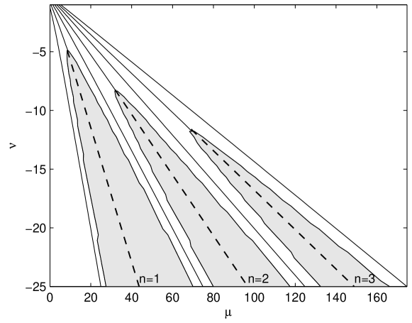
Figure 9: A contour plot of the mean occupation $\overline{n}$ with respect to the Lagrange multipliers $\mu$ and $\nu$ reveals the Mott lobes for commensurate occupations, shown for $\overline{n}=1$, $2$, $3$, where the solutions to (104) are degenerate with respect to $\mu$, indicating the incompressibility of the phase. The Mott insulator phase does not exist for incommensurate occupations as shown by the remaining curves at $\overline{n}=0.5$, $1.5$, $2.5$ and $3.5$ from left to right in the figure. The dashed lines represent possible (non-degenerate) trajectories for the Mott insulator phase as discussed in section 6.1.1.

The correlation and mean-field can then be written respectively in terms of the vector quadratic forms

$$\langle V\rangle=\mathbf{C}^{T}A_{V}\mathbf{C}$$ (94)

$$\langle X\rangle=\mathbf{C}^{T}A_{X}\mathbf{C}$$ (95)

where the construction of matrices $A_{V}$ and $A_{X}$ follows directly from equations (53) and (84). In particular,

$$A_{V}=\left(\begin{array}[]{c|c|cc|cc|ccc|c}0&\lx@intercol\hfil 0\hfil\lx@intercol&0&\lx@intercol\hfil 0\hfil\lx@intercol&0&\lx@intercol\hfil 0\hfil\lx@intercol&0&0&\lx@intercol\hfil 0\hfil\lx@intercol&\\ \cline{1-2}\cr 0&1&0&\lx@intercol\hfil 0\hfil\lx@intercol&0&\lx@intercol\hfil 0\hfil\lx@intercol&0&0&\lx@intercol\hfil 0\hfil\lx@intercol&\\ \cline{2-4}\cr\lx@intercol\hfil 0\hfil\lx@intercol&0&0&2\sqrt{2}&0&\lx@intercol\hfil 0\hfil\lx@intercol&0&0&\lx@intercol\hfil 0\hfil\lx@intercol&\\ \lx@intercol\hfil 0\hfil\lx@intercol&0&0&0&0&\lx@intercol\hfil 0\hfil\lx@intercol&0&0&\lx@intercol\hfil 0\hfil\lx@intercol&\\ \cline{3-6}\cr\lx@intercol\hfil 0\hfil\lx@intercol&\lx@intercol\hfil 0\hfil\lx@intercol&0&0&2&2\sqrt{3}&0&0&\lx@intercol\hfil 0\hfil\lx@intercol&\\ \lx@intercol\hfil 0\hfil\lx@intercol&\lx@intercol\hfil 0\hfil\lx@intercol&0&0&0&0&0&0&\lx@intercol\hfil 0\hfil\lx@intercol&\\ \cline{5-9}\cr\lx@intercol\hfil 0\hfil\lx@intercol&\lx@intercol\hfil 0\hfil\lx@intercol&0&\lx@intercol\hfil 0\hfil\lx@intercol&0&0&0&2\sqrt{6}&0&\\ \lx@intercol\hfil 0\hfil\lx@intercol&\lx@intercol\hfil 0\hfil\lx@intercol&0&\lx@intercol\hfil 0\hfil\lx@intercol&0&0&0&0&4&\\ \lx@intercol\hfil 0\hfil\lx@intercol&\lx@intercol\hfil 0\hfil\lx@intercol&0&\lx@intercol\hfil 0\hfil\lx@intercol&0&0&0&0&0&\\ \cline{7-10}\cr\lx@intercol\hfil\hfil\lx@intercol&\lx@intercol\hfil\hfil\lx@intercol&\lx@intercol\hfil\hfil\lx@intercol&\lx@intercol\hfil\hfil\lx@intercol&\lx@intercol\hfil\hfil\lx@intercol&\lx@intercol\hfil\hfil\lx@intercol&\lx@intercol\hfil\hfil\lx@intercol&\lx@intercol\hfil\hfil\lx@intercol&&\ddots\end{array}\right)$$ (96)

and

$$A_{X}=\left(\begin{array}[]{c|c|cc|cc|ccc|c}0&\lx@intercol\hfil 1\hfil\lx@intercol&0&\lx@intercol\hfil 0\hfil\lx@intercol&0&\lx@intercol\hfil 0\hfil\lx@intercol&0&0&\lx@intercol\hfil 0\hfil\lx@intercol&\\ \cline{1-2}\cr 0&0&1&\lx@intercol\hfil\sqrt{2}\hfil\lx@intercol&0&\lx@intercol\hfil 0\hfil\lx@intercol&0&0&\lx@intercol\hfil 0\hfil\lx@intercol&\\ \cline{2-4}\cr\lx@intercol\hfil 0\hfil\lx@intercol&0&0&0&\sqrt{2}&\lx@intercol\hfil 0\hfil\lx@intercol&0&0&\lx@intercol\hfil 0\hfil\lx@intercol&\\ \lx@intercol\hfil 0\hfil\lx@intercol&0&0&0&1&\lx@intercol\hfil\sqrt{3}\hfil\lx@intercol&0&0&\lx@intercol\hfil 0\hfil\lx@intercol&\\ \cline{3-6}\cr\lx@intercol\hfil 0\hfil\lx@intercol&\lx@intercol\hfil 0\hfil\lx@intercol&0&0&0&0&\sqrt{2}&\sqrt{3}&\lx@intercol\hfil 0\hfil\lx@intercol&\\ \lx@intercol\hfil 0\hfil\lx@intercol&\lx@intercol\hfil 0\hfil\lx@intercol&0&0&0&0&0&1&\lx@intercol\hfil 2\hfil\lx@intercol&\\ \cline{5-9}\cr\lx@intercol\hfil 0\hfil\lx@intercol&\lx@intercol\hfil 0\hfil\lx@intercol&0&\lx@intercol\hfil 0\hfil\lx@intercol&0&0&0&0&0&\\ \lx@intercol\hfil 0\hfil\lx@intercol&\lx@intercol\hfil 0\hfil\lx@intercol&0&\lx@intercol\hfil 0\hfil\lx@intercol&0&0&0&0&0&\\ \lx@intercol\hfil 0\hfil\lx@intercol&\lx@intercol\hfil 0\hfil\lx@intercol&0&\lx@intercol\hfil 0\hfil\lx@intercol&0&0&0&0&0&\\ \cline{7-10}\cr\lx@intercol\hfil\hfil\lx@intercol&\lx@intercol\hfil\hfil\lx@intercol&\lx@intercol\hfil\hfil\lx@intercol&\lx@intercol\hfil\hfil\lx@intercol&\lx@intercol\hfil\hfil\lx@intercol&\lx@intercol\hfil\hfil\lx@intercol&\lx@intercol\hfil\hfil\lx@intercol&\lx@intercol\hfil\hfil\lx@intercol&&\ddots\end{array}\right)$$ (97)

The constraints (89)–(6) can then be written as

$$\phi_{1}=\mathbf{C}^{T}S\mathbf{C}-1=0$$ (98)

$$\phi_{2}=\textstyle\frac{1}{2}\mathbf{C}^{T}\,S\,D\,\mathbf{C}-\overline{n}=0$$ (99)

$$\phi_{3}=\textstyle\frac{1}{4}\mathbf{C}^{T}\,S\,D^{\prime}\,\mathbf{C}-\overline{n^{2}}=0$$ (100)

where $S$, $D$ and $D^{\prime}$ are diagonal matrices with elements given by

$$S_{NN^{\prime}pp^{\prime}}=\delta_{NN^{\prime}}\,\delta_{pp^{\prime}}\,(2-\delta_{p0})$$ (101)

$$D_{NN^{\prime}pp^{\prime}}=\delta_{NN^{\prime}}\,\delta_{pp^{\prime}}\,N$$ (102)

$$D^{\prime}_{NN^{\prime}pp^{\prime}}=\delta_{NN^{\prime}}\,\delta_{pp^{\prime}}\,(N^{2}\!+\!p^{2})$$ (103)

with the usual Kronecker delta function. Using these definitions, equation (92) can then be written in matrix form as

$$(S^{-1/2}AS^{-1/2}+S^{1/2}BS^{-1/2})\mathbf{u}=\lambda\mathbf{u}$$ (104)

where

$$\mathbf{u}=S^{1/2}\mathbf{C}$$ (105)

$$A=A_{V}+A_{V}^{T}+(2d\!-\!1)\langle X\rangle(A_{X}+A_{X}^{T})$$ (106)

$$B=\mu\,D+\textstyle\frac{1}{2}\,\nu\,D^{\prime}$$ (107)

   

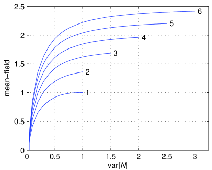
(a) Commensurate

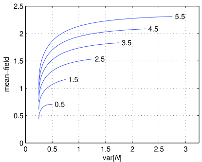
(b) Incommensurate

Figure 10: Mean-field as a function of number variance for commensurate (a) and incommensurate (b) occupations. In contrast to the one site approximation, in the commensurate case the Mott insulator phase with vanishing mean-field can occur for a non-zero number variance.

           

(a) Mean-field, d=1

(b) Intersite correlation, d=1

(c) Mean-field, d=2

(d) Intersite correlation, d=2

(e) Mean-field, d=3

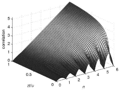
(f) Intersite correlation, d=3

Figure 11: Ground state results for the Bose-Hubbard model in the two site mean-field approximation. The mean-field and intersite correlations are shown as a function of the mean site occupation $\overline{n}$ and the relative interaction strength $zt/u$. A non-zero mean-field represents the superfluid regime. The mean-field is zero below a critical value $(zt/u)_{c}$ for commensurate occupations, indicating the onset of the Mott insulator phase. The intersite correlations are non-zero everywhere except for commensurate occupations in the limit of no tunnelling where $zt/u=0$. The results are qualitatively similar for 1, 2, and 3 dimensional lattices. However, a feature of the $d=1$ phase diagram is the weak suppression of the mean-field at half-integer occupations, which is seen more seen more clearly in Fig.13. This may be an artefact of the two site approximation and requires further study.

           

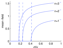
(a) Mean-field, $d=1$

(b) Mean-field, $d=2$

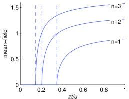
(c) Mean-field, $d=3$

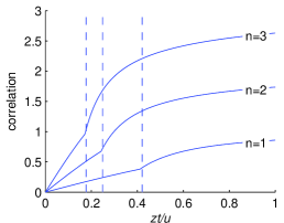
(d) Correlation, $d=1$

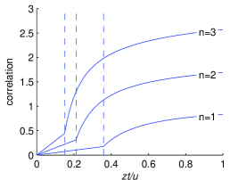
(e) Correlation, $d=2$

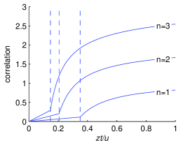
(f) Correlation, $d=3$

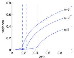
(g) Variance, $d=1$

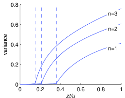
(h) Variance, $d=2$

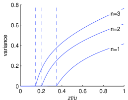
(i) Variance, $d=3$

Figure 12: $d=1$, $2$, $3$ results: mean-field, intersite correlation and variance for commensurate occupations of $\overline{n}=1$, $2$, $3$. The dashed vertical lines indicate the corresponding positions (from left to right) of the phase boundary between the superfluid and Mott insulator phases as calculated using the pertubation theory outlined in section 6.3

This can be made linear in $\mathbf{u}$ (and therefore $\mathbf{C}$) when the mean-field term $\langle X\rangle$ in (106) is treated as a free parameter $x$; the resulting eigenvalue equation is solved iteratively in $x$ so that it is self-consistent with the calculated mean-field $\langle X\rangle=\mathbf{C}^{T}A_{X}\mathbf{C}$. The eigenvector solution $\mathbf{u}$ which maximizes $F$ at each iteration is nonnegative; in fact the nonnegative eigenvector, the maximizing solution, belongs to the maximum eigenvalue as we now show.

6.0.2 Determining the maximising solution

To see why this is the case we need to invoke the Perron-Frobenius theorem for nonnegative matrices [10]. We first note that the $r\times r$ matrix $G=S^{-1/2}AS^{-1/2}+S^{1/2}BS^{-1/2}$ in equation (104) is nonnegative everywhere except along the leading diagonal where negative values are possible when either $\mu$ or $\nu$ (or both) are negative. It is then always possible to construct a matrix $G^{\prime}=G+\gamma I_{r}$ that is nonnegative everywhere for a sufficiently large $\gamma$, $I_{r}$ being the $r\times r$ identity matrix.

The eigenvectors of $G^{\prime}$ and $G$ are clearly the same with the eigenvalues of $G^{\prime}$ given by $\lambda^{\prime}_{i}=\lambda_{i}+\gamma$ where $\lambda_{i}$ is the $i$th eigenvalue of $G$ corresponding to the $i$th eigenvector. The Perron-Frobenius theorem states that the spectral radius $\rho$ of a nonnegative matrix is an eigenvalue corresponding to a nonnegative eigenvector. That is, $\rho(G^{\prime})$ is the eigenvalue with the desired nonnegative solution. We can relate this to the maximum eigenvalue of $G$ when $\gamma$ simultaneously satisfies the following two conditions:

1. $\gamma\geq|\textrm{min}(G)|$ so that $G^{\prime}$ is nonnegative

2. $\gamma\geq|\textrm{min}(\lambda_{i})|$ so that all $\lambda^{\prime}_{i}\geq 0$ and $\textrm{max}(\lambda_{i})+\gamma$ is necessarily the spectral radius of $G^{\prime}$

For any bounded matrix $G$ it is always possible to select such a value of $\gamma$; we can therefore associate the correct solution for $C_{N,p}$ with the maximum eigenvalue of (104) which returns a self-consistent mean-field.

6.1 The ground state solution

The general procedure for finding the ground state solution follows the method used in the one site formulation (see section 4). In particular, at a given mean occupation $\overline{n}$, (104) determines a locus of solutions which can be expressed as a function of number variance. Therefore, at a given $t/u$ and $n$, the two site energy can be reparameterized in terms of number variance; finding the ground state phase diagram then only requires the minimization of the energy with respect to variance. In practice to perform this procedure efficiently, it is useful to first calculate a set of solution states covering a suitable variance range, which act as initial conditions in the final minimisation step.

In the results presented here, this was achieved by fixing $\overline{n}$ and initially choosing a large value for the variance corresponding to the superfluid regime (specifically ${\rm var}[N]=\overline{n}$ for $\overline{n}\leq 1$ and ${\rm var}[N]=\overline{n}/2$ for $\overline{n}\geq 1$). The corresponding state was found by solving equation (104) using the initial values $x_{0}=5$, $\mu_{0}=2$ and $\nu_{0}=-1$, which was found to be sufficient for the range of parameters considered here. A lower variance was then selected and its corresponding state was calculated, by using the previous solution to determine the initial conditions. By iteration it was then possible to find solutions efficiently over a broad variance range.

However, although this general procedure works well for most of the parameter space, it fails to converge (to a sufficient accuracy) in two limiting cases: for Mott-insulator states where the mean-field is zero and there is degeneracy; and in the limit of the lowest possible variance, ${\rm var}[N]=\delta\overline{n}(1-\delta\overline{n})$, corresponding to the localized region where the Lagrange multipliers diverge at the solution. It is therefore necessary to consider these cases separately.

6.1.1 Calculating Mott states

For commensurate occupations and below a critical value for the variance, the system is in the Mott insulator state corresponding to a vanishing mean-field. In this case, the above approach is numerically unstable for two reasons. Firstly, the algorithm fails to correctly converge to a zero mean-field since the search direction cannot be determined. Secondly, the system states become highly degenerate in $\mu$ in the Mott insulator state (corresponding to a incompressible phase) which further prevents convergence (with respect to $\mu$).

These problems are circumvented respectively by the following adjustments to the general procedure. Firstly, explicitly setting the free-parameter $x$ to zero in the equation (104), ensures that any solution is self-consistent in the mean-field; this can be seen to be case by considering how the mean-field term appears in the eigenvalue equation (see (94) and (106) in particular). Secondly, setting $\mu=-r\,\nu$ for a suitably chosen quantity $r$, restricts the parameter space to the degenerate region, so that $\overline{n}$ remains fixed while ${\rm var}[N]\rightarrow 0$ in the limit $\nu\rightarrow\infty$. These trajectories are illustrated by the dashed curves in Fig.9. By enforcing this relationship between $\mu$ and $\nu$, we can therefore probe the Mott insulator states accurately.

6.1.2 Solutions in the limit of zero tunneling

Considering (83) in the limit of zero tunneling where $t/u\rightarrow 0$, the ground state is clearly determined by states of the lowest possible variance. In this case, we found the method of Lagrange multipliers leads to poor convergence as the Lagrange multipliers diverge at the solution. We therefore consider a more direct method whereby we minimize the two site energy in terms of a reduced parameter space, which correspond to the lowest allowed variance (${\rm var}[N]=\delta n(1-\delta n)$) for a given mean occupation $\overline{n}$.

Recall the lowest variance state is given by equation (75); in this basis, the hopping energy (88) is given by

$$F=\beta/2([{\overline{n}}]+1)(1+(2d-1)(\sqrt{\alpha}+\sqrt{\gamma})^{2})$$ (108)

The constraints (normalization, fixed $\overline{n}$ and fixed variance) can be given as a set of linear equations

$$\alpha+\beta+\gamma = 1$$

$$[{\overline{n}}]\alpha+([{\overline{n}}]\!+\!\textstyle\frac{1}{2})\beta+([{\overline{n}}]\!+\!1)\gamma = \overline{n}$$

$${[{\overline{n}}]}^{2}\alpha+({[{\overline{n}}]}^{2}\!+\![{\overline{n}}]\!+\!\textstyle\frac{1}{2})\beta+({[{\overline{n}}]}^{2}\!+\!2[{\overline{n}}]\!+\!1)\gamma = {\rm var}[N]+\overline{n}^{2}$$ (109)

which when written as $Ax=b$, admits solutions of the form $x=x_{0}+\kappa\,\textrm{nullspace}[A]$ where we have taken

$$x_{0}=\begin{array}[]{|c|}\alpha\\ \beta\\ \gamma\end{array}=\begin{array}[]{|c|}[\overline{n}]+1-\overline{n}\\ 0\\ \overline{n}-[\overline{n}]\end{array}$$ (110)

as a solution of the homogenous system $Ax=0$. There is an additional requirement on $\kappa$ that the coefficients are bounded with $0\leq\alpha\leq 1$, $0\leq\beta\leq 2$ and $0\leq\gamma\leq 1$. For a given occupation $\overline{n}$ and dimension $d$, we can then maximise the hopping energy (108) with respect to the remaining free parameter $\kappa$. The ground state phase diagram is then calculated easily for the case where $zt/u=0$; the resulting mean-field and intersite correlation are shown in figures 13(a) and 13(b) respectively.

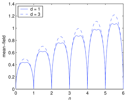
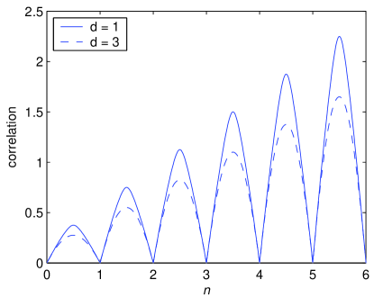
Figure 13: The mean-field (a) and intersite correlation (b) using a reduced basis of three states in the limit of zero tunelling ($zt/u=0$) for $d=1$, $3$. The methodology is outlined in section 6.1.2. A feature of the $d=1$ case is the weak supression of the mean-field around half-integer occupations. The $d=2$ results, which been omitted for clarity, are very close to the $d=3$ case.

6.1.3 Numerical Solutions

Numerical calculations were performed using a state space truncated with $N\leq 20$, corresponding to 121 coefficients $C_{N,\,p}$. The MATLAB function fsolve was used to find the self-consistent solution, for a given $\overline{n}$ and ${\rm var}[N]$, by supplying the function with suitable initial values $x_{0}$, $\mu_{0}$ and $\nu_{0}$ for the mean-field and Lagrange multipliers.

6.2 Results

Using the calculated states with maximum tunneling energy, the two site energy (83) was then minimized with respect to ${\rm var}[N]$ for a given $\overline{n}$ and $Z/u$. The results of this calculation are shown in Figs. 11(a)-(f) for arbitrary mean occupations. To investigate the superfluid to Mott-insulator transition more clearly, these results have also been reproduced for commensurate occupations in Figures 12(a)–(i).

This ground state phase diagram is qualitatively similar to the results for the one site model (Fig.2); the most important feature of both models is the vanishing of the mean-field for commensurate occupations above the critical transition point $\overline{u}_{c}$, corresponding to the Mott insulator phase. Note that the Mott insulator to superfluid transition is clearly reproduced for commensurate mean occupations, an improvement over the corresponding two site Q-function approximation (section 5) which can be attributed to the exact treatment of the intersite correlations in the present treatment. We now consider a simple perturbative expansion from which the position of the phase transition boundary can be easily calculated for the two site formulation.

6.3 Calculating the phase transition boundary

Following the one-site case, we consider the following states near the transition with commensurate occupation $\overline{n}$:

$$|s\rangle=\sqrt{1-\alpha-2\beta}\,|\overline{n},\overline{n}\rangle+\sqrt{\frac{\alpha}{2}}(|\overline{n}-1,\overline{n}+1\rangle+|\overline{n}+1,\overline{n}-1\rangle)$$

$$+\sqrt{\frac{\beta}{2}}\bigg{(}|\overline{n},\overline{n}-1\rangle+|\overline{n}-1,\overline{n}\rangle+|\overline{n},\overline{n}+1\rangle+|\overline{n}+1,\overline{n}\rangle\bigg{)}$$ (111)

This state is a superposition of the minimum set of number states that give a non-zero mean-field and intersite correlation. The coefficients have been chosen to satisfy normalization and a fixed commensurate occupation $\overline{n}$. The corresponding variance on one site is given by ${\rm var}[N]=\alpha+\beta$. Note that $|s\rangle$ represents a perturbation in $\alpha$ and $\beta$ from the Mott insulator phase. With this state the intersite correlation (86) is given by

$$\langle V\rangle=\sqrt{2(1-\alpha-2\beta)\alpha}\,\sqrt{\overline{n}(\overline{n}+1)}+\frac{\beta}{2}(2\overline{n}+1)$$ (112)

and the mean-field (84) is

$$\langle X\rangle=\sqrt{\frac{\beta}{2}}\left(\sqrt{1-\alpha-2\beta}+\sqrt{\frac{\alpha}{2}}\right)(\sqrt{\overline{n}}+\sqrt{\overline{n}+1})$$ (113)

In the ground state, the phase transition occurs for the minimum two site energy (83); clearly this occurs with respect to the state (6.3) when $\partial{E_{12}}/\partial{\alpha}=0$ and $\partial{E_{12}}/\partial{\beta}=0$ are both satisfied. Moreover the phase transition occurs for $\beta=0$ where the mean-field is zero. That is,

$$0=\frac{\partial{E}}{\partial{\alpha}}\bigg{|}_{\beta=0}=\left(\frac{u}{t}\right)-\frac{\sqrt{\overline{n}(1+\overline{n})}(1-2\alpha)}{\sqrt{2\alpha(1-\alpha)}}$$ (114)

$$0=\frac{\partial{E}}{\partial{\beta}}\bigg{|}_{\beta=0} = \left(\frac{u}{t}\right)-\textstyle\frac{1}{2}(1+2\overline{n})$$ (115)

$$-\textstyle\frac{1}{2}(2d-1)(\sqrt{\overline{n}}+\sqrt{\overline{n}+1})^{2}(\sqrt{1-\alpha}+\sqrt{\alpha/2})^{2}$$

$$+\frac{\sqrt{2\alpha\overline{n}(\overline{n}+1)}}{\sqrt{1-\alpha}}$$

Numerically solving these equations leads to the results shown in table 1. Note that in the non-physical limit of $d\!\rightarrow\!\infty$ the variance at the transtion is ${\rm var}[N]=\alpha=0$. Considering equation (115) the transition then occurs at $\overline{U}_{c}=2(u/2dt)_{c}=(\sqrt{\overline{n}}+\sqrt{\overline{n}+1})^{2}$, the same value as in the one-site model. This is not unexpected as the intersite correlation $\langle V\rangle$ becomes negligible compared with the mean-field contribution in the Hamiltonian (40).

$d$	$\overline{n}=1$	$\overline{n}=2$	$\overline{n}=3$
$1$	$4.75$	$8.02$	$11.26$
$2$	$5.56$	$9.43$	$13.27$
$3$	$5.71$	$9.69$	$13.63$
$10$	$5.82$	$9.88$	$13.90$
$10^{6}$	$5.83$	$9.90$	$13.93$

Table 1: Critical value $\overline{U}_{c}$ calculated for two site mean-field approximation using a perturbation expansion around the Mott Insulator state

There are some notable differences between the one and two site mean-field approximations, which we discuss here. In particular, the inclusion of intersite correlations in the two site Hamiltonian, results in a non-zero number variance even in the Mott insulator phase where the mean-field vanishes; this can be seen in Figs. 10 and 12. This contrasts with the one site results (see Fig. 7) where the mean-field and number variance are identically zero. Moreover, for the two site model the calculated transition points $\overline{U}_{c}$, as shown in table 1, occur at lower values than for the one site model. In particular, for $\overline{n}=1$ and $d=1$, the two site model yields $\overline{U}_{c}=4.75$, whereas the one site model gives $\overline{U}_{c}=5.83$.

These differences are most pronounced for the $d=1$ case where the mean-field approximation is no longer valid, as has also been noted elsewhere [8]. At higher dimensions ($d=2$, $3$), where the mean-field approximation is more accurate, the number variance is close to zero in the Mott phase and the calculated transition points for the one and two site models are close. It is expected that in the (non-physical) limit of infinite lattice dimensionality, the one and two site results will converge.

6.4 Comparison to other work

The results for the two site Hamiltonian given in the previous section clearly demonstrate a partial shift to lower values $\overline{U}_{c}$ (ie. a weaker lattice) when compared to the one site results. This shift can be attributed to the inclusion of intersite correlations in the model. To compare with our results with those reported elsewhere it is useful to refer to table 2.

For the $d=1$ case, numerically exact schemes, with Density Matrix Renormalization Group (DMRG) and Quantum Monte-Carlo (QMC) simulations, predict a much lower value for the phase transition point $\overline{U}_{c}$ in the Bose-Hubbard model. Using the DMRG technique with the infinite-system algorithm, the transition point for $\overline{n}=1$ and $d=1$ has been reported as $\overline{U}_{c}=1.68$ [11] and $\overline{U}_{c}=1.81$ [12]. Using the more accurate finite-system algorithm, the same transition has been reported as $\overline{U}_{c}=1.92$ [13] and $\overline{U}_{c}=1.68$ [14]. Similarly, for QMC simulations without lattice disorder, the transition has been reported as $\overline{U}_{c}=2.33$ [15]. Also, pertubative expansions using defect states have yielded similar results to the that of the QMC technique in one dimension. In particular, the above transition has been reported as $\overline{U}_{c}=2.33$ [16] and $\overline{U}_{c}=2.04$ [17].

Method	Position of phase transition boundary for $d=1$, $n=1$ (unless otherwise stated)	Authors	Reference
Mean-field approximation using second order perturbation expansion	$\overline{U}_{c}=2n+1+\sqrt{(2n+1)^{2}-1}$, $\overline{n}=1$: $\overline{U}_{c}=5.83$	Oosten et al.	[4]
Mean-field theory using variational approach	$\overline{U}_{c}=2.0$	Amico and Penna	[18]
Mean-field theory using variational approach	$\overline{n}=1$: $\overline{U}_{c}=5.83$	Sheshadri et al.	[9]
Perturbative expansion using defect (particle/hole) states	$d=1$, $\overline{n}=1$: $\overline{U}_{c}=2.33$; $d=2$, $\overline{n}=1$: $\overline{U}_{c}=3.68$	Freericks and Monien	[16]
Perturbative expansion using defect (particle/hole) states	$\overline{U}_{c}=2.04$ (see table in reference for further calculated values at different $d$ and $n$)	Freericks and Monien	[17]
Quantum Monte-Carlo	$\overline{U}_{c}=2.33$ (without disorder)	Batrouni and Scalettar	[15]
DMRG with infinite-system algorithm	$\overline{U}_{c}=1.68$	Pai et al.	[11]
DMRG with infinite-system algorithm	$\overline{U}_{c}=1.81$ (without nearest-neighbour interactions)	Kuhner and Monien	[12]
DMRG with finite-system algorithm	$\overline{U}_{c}=1.68$ (without nearest-neighbour interactions)	Kuhner et al.	[14]
DMRG with finite-system algorithm	$\overline{U}_{c}=1.92$ (for zero disorder)	Rapsch et al.	[13]

Table 2: The calculated boundary of the Superfluid to Mott-insulator phase boundary as determined from the Bose-Hubbard model as solved using various methods in the literature.

7 Conclusions

We have presented two model Hamiltonians for the Bose-Hubbard model using two different mean-field approximations. The simpler one site model treats all intersite correlations using a mean-field approximation that decouples the problem into the sum of one site Hamiltonians. The second model is a two site extension where intersite correlations between two adjacent sites are explicitly included while treating interactions with neighbouring sites using the mean-field approximation. Each model has been tackled using two methodologies: a treatment in terms of a Q-function representation; and a numerically exact method using either the one or two site states.

In the case of the one site Hamiltonian, we find the Q-function representation agrees well with the numerically exact treatment, but can be solved at a fraction of the computational cost. For the two site Hamiltonian, the Q-function gives a good qualitative description but does not give a clear Mott insulator to superfluid transition due to limitations of the parameterization on two sites. It is encouraging, however, that the Q-function approach gives the intersite correlations accurately when compared with the two site exact solution. In contrast to the Q-function approach, the two site exact solution yields a well-defined phase transition for commensurate mean occupations. In this case, the critical relative interaction strength $\overline{U}_{c}$ is smaller (corresponding to a weaker lattice strength) for all commensurate values of $\overline{n}$ than for the one site model; this shift is most pronounced for a one dimensional lattice.

What emerges from the Q-function approach is that the quantum mechanical constraints play a primary role in determining the ground state results for the Bose-Hubbard model. This is most clearly illustrated by the one site formulation where the results are determined by the uncertainty relation in two forms: a restriction on the minimum variance permitted by the quantum state; and a relation between the number and phase fluctuations. In particular, the onset of the Mott insulator phase is characterized by supression of number fluctuations at the lower bound of the variance constraint.

Exact numerical results with QMC or DMRG simulations on finite one dimensional lattices by other authors indicate the actual position of the superfluid to Mott insulator transition occurs for an even lower value of $\overline{U}_{c}$ than is calculated by our two site model. It is expected that if we were to extend our formalism to explicitly include the interactions between three or more sites, the predicted value $\overline{U}_{c}$ would shift to lower values in line with these other treatments. However, this remains a computationally difficult problem due to the dramatic increase in the size of the Hilbert space of the problem when more sites are included.

8 Acknowlegments

The authors would like to thank D. Jaksch and P. Zoller (of Institut für theoretische Physik, Universtität Innsbruck, Austria) for useful discussions.

References

Appendix A Values of parameters in particlar cases.

To fit the kinds of distribution in Fig.3 we determine the parameters $v$, $\sigma$ and $c$ by fitting the moments $\langle{a}\rangle$, $\langle{a}{a}^{\dagger}\rangle$ and $\langle{a}{a}{a}^{\dagger}{a}^{\dagger}\rangle$.

Parameters for a number state

The exact values for the quantities (10–14) in the case of a number state $|m\rangle$ are

$$\langle{a}\rangle = 0$$ (116)

$$\langle{a}{a}^{\dagger}\rangle = m+1$$ (117)

$$\langle{a}{a}\rangle = 0$$ (118)

$$\langle{a}{a}{a}^{\dagger}\rangle = 0$$ (119)

$$\langle{a}{a}{a}^{\dagger}{a}^{\dagger}\rangle = (m+1)(m+2)$$ (120)

leading to the choice

$$v^{4} = m^{2}+{3\over 2}m+{1\over 2}$$ (121)

$$\sigma = m+1-\sqrt{m^{2}+{3\over 2}m+{1\over 2}}$$ (122)

$$\approx {1/4}\quad\mbox{ as $m\to\infty$}$$ (123)

$$c = 0.$$ (124)

The two quantities (118,119) are given exactly by this choice.

Parameters for a superposition of two number states

For an equal superposition of the kind (ii)) that

$$v^{4} = n^{2}+{n\over 2}-{1\over 8}$$ (125)

$$\sigma = n+{1\over 2}-\sqrt{n^{2}+{n\over 2}-{1\over 8}}$$ (126)

$$c = {{\sqrt{n}}\over 2v}.$$ (127)

The exact computation of the quantities (10–14) yields in this case

$$\langle{a}\rangle = {1\over 2}\sqrt{n}$$ (128)

$$\langle{a}{a}^{\dagger}\rangle = n+{1\over 2}$$ (129)

$$\langle{a}{a}\rangle = 0$$ (130)

$$\langle{a}{a}{a}^{\dagger}\rangle = {1\over 2}(n+1)\sqrt{n}$$ (131)

$$\langle{a}{a}{a}^{\dagger}{a}^{\dagger}\rangle = (n+1)^{2}$$ (132)

The first, second and last of these are fitted exactly, leading to the approximate values

$$\langle{a}{a}\rangle \approx (v^{2}+\sigma)c^{4}$$ (133)

$$= \left(n+{1\over 2}\right){n^{2}\over 16(n^{2}+n/2-1/8}$$

$$\langle{a}{a}{a}^{\dagger}\rangle \approx (v^{3}+3\sigma v)c$$

$$= {1\over 2}\sqrt{n}\left(3\left(n+{1\over 2}\right)-2\sqrt{n^{2}+n/2-1/8}\right)$$

Even for $n=1$ these are very tolerable approximations; (133) is diminished by comparison with $\langle{a}{a}^{\dagger}\rangle$ by a factor of $c^{4}\approx 0.045$, compared to the exact value of 0. For large $n$ (A) becomes equal to the true value (131), and even for $n=1$ the true and the model results differ by less than 8%.

Parameters for a coherent state

For a coherent state $|\beta\rangle$, where $\beta\equiv m$ is taken to be real, the quantities take the form

$$\langle{a}\rangle = \beta$$ (135)

$$\langle{a}{a}^{\dagger}\rangle = \beta^{2}+1$$ (136)

$$\langle{a}{a}\rangle = \beta^{2}$$ (137)

$$\langle{a}{a}{a}^{\dagger}\rangle = \beta(\beta^{2}+2)$$ (138)

$$\langle{a}{a}{a}^{\dagger}{a}^{\dagger}\rangle = \beta^{4}+4\beta^{2}+2$$ (139)

from which we can compute

$$v^{4} = \beta^{4}+\beta^{2}+{1\over 2}$$ (140)

$$\sigma = \beta^{2}=1-\sqrt{\beta^{4}+\beta^{2}+{1\over 2}}$$ (141)

$$c = {\beta\over v}\approx 1-{1\over 2\beta^{2}}\quad\mbox{ as $\beta\to\infty$}$$ (142)

It is easy to check that for large $\beta$ the quantities (137,138) are correctly given, and they are of course correct for $\beta=0$. For $\beta=1$, we find that $\langle{a}{a}\rangle=0.8$ instead of the exact value of 1, and $\langle{a}{a}{a}^{\dagger}\rangle=2.84$, instead of the exact value of 3.

Appendix B A rigorous lower bound on the energy

As a spinoff from our methodology of section 3, we find that we can also develop a rigorous lower bound for the energy as a function of the mean-field, and we can evaluate the predictions given by assuming the lower bound is equal to the ground-state energy.

To see this we note the mean energy, which is given by (29) in the mean-field approximation, is parametrized by number variance ${\rm var}[N]$ and the mean-field $\langle X\rangle$. Then we know that ${\rm var}[N]$ satisfies the two inequalities (20) and (24), which we can combine together as

$${\rm var}[N] \geq \max\left({\langle X\rangle^{2}\over 4\langle Y^{2}\rangle},\delta n(1-\delta n)\right).$$ (143)

We can develop a lower bound on $\langle Y^{2}\rangle$ by noting that

$$\langle Y^{2}\rangle = n-{1\over 2}-\langle X^{2}\rangle\leq n-{1\over 2}-\langle X\rangle^{2},$$ (144)

so that we can deduce from (143) that

$${\rm var}[N] \geq \max\left({\langle X\rangle^{2}\over 4(n-{1\over 2}-\langle X\rangle^{2})},\delta n(1-\delta n)\right),$$ (145)

and that the mean energy (29) satisfies the lower bound

$$\langle E\rangle \geq -Z\langle X\rangle^{2}+u\left\{2+n^{2}+3n+\max\left({\langle X\rangle^{2}\over 4(n-{1\over 2}-\langle X\rangle^{2})},\delta n(1-\delta n)\right)\right\}.$$ (146)

This bound is parametrized by the mean-field $\langle X\rangle$ only, so the rigorous lower bound is given by the value, $X_{\rm min}(u,n)$, of $\langle X\rangle$ which gives the minimum value, $E_{\rm min}(u,n)$, the right hand side of (146), and subject to the restriction that $\langle X\rangle\leq\sqrt{n-1}$ (the equality holding for a coherent state). These are easy to evaluate, and resulting chemical potential and mean-field are plotted in Fig.14. The results are less accurate than the phase space method (see Fig.5), but are still surprisingly good.

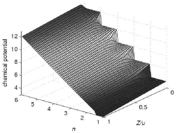
Figure 14: Ground state phase diagram calculated using rigorous lower bound on energy (146) in Q-function representation

References

- [1] D. Jaksch, C. Bruder, J. I. Cirac, C. W. Gardiner, and P. Zoller. Cold bosonic atoms in optical lattices. Phys. Rev. Lett., 81(15):3108, October 1998.
- [2] Markus Greiner, Olaf Mandel, Tilman Esslinger, Theodor W. Hänsch, and Immanuel Bloch. Quantum phase transition from a superfluid to a Mott insulator in a gas of ultracold atoms. Nature, 415:39, 2002.
- [3] Ana Maria Rey, Keith Burnett, Robert Roth, Mark Edwards, Carl J. Williams, and Charles W. Clark. Bogoliubov approach to superfluidity of atoms in an optical lattice. J. Phys. B., 36:825, 2003.
- [4] D. van Oosten, P. van der Straten, and H. T. C. Stoof. Quantum phases in an optical lattice. Phys. Rev. A, 63(053601), 2001.
- [5] Matthew P.A. Fisher, Peter B. Weichman, G. Grinstein, and Daniel S. Fisher. Boson localization and the superfluid-insulator transition. Physical Review B, 40(15):546, July 1989.
- [6] S. Sachdev. Quantum Phase Transitions. Cambridge University Press, 1990, 2000.
- [7] C. W. Gardiner and P. Zoller. Quantum Noise. Springer, 1999.
- [8] Wilhelm Zwerger. Mott-Hubbard transition of cold atoms in optical lattices. J. Opt. B: Quantum Semiclass. Opt., 5:S9, 2003.
- [9] K. Sheshadri, H.R. Krishnamurthy, R. Pandit, and T.V. Ramakrishnan. Superfluid and Insulating Phases in an Interacting-Boson Model: Mean-Field Theory and the RPA. Europhys. Lett., 22(4):257, 1993.
- [10] C.R. MacCluer. The Many Proofs and Applications of Perron’s Theorem. Siam Review, 42(3):487, 2000.
- [11] Ramesh V. Pai, Rahul Pandit, H.R. Krishnamurthy, and S. Ramasesha. One-dimensional Disordered Bose Hubbard Model: A Density-Matrix Renormalization Group Study. Physical Review Letters, 76(16):2937, 1996.
- [12] T.D. Kühner and H. Monien. Phases of the one-dimensional Bose-Hubbard model. Physical Review B, 58(22):14741, 1998.
- [13] S. Rapsch, U. Schollwöck, and W. Zwerger. Density matrix renormalization group for disordered bosons in one dimension. Europhys. Lett., 46:559, 1999.
- [14] Till D. Kühner, Steven R. White, and H. Monien. One-dimensional Bose-Hubbard model with nearest-neighbor interaction. Physical Review B, 61(18):12474, 2000.
- [15] Ghassan George Batrouni and Richard T. Scalettar. World-line quantum Monte Carlo algorithm for a one-dimensional Bose model. Physical Review B, 46(14):9051, 1992.
- [16] J.K. Freericks and H. Monien. Phase diagram of the Bose-Hubbard model. Europhys. Lett., 26(7):545, 1994.
- [17] J.K. Freericks and H. Monien. Strong-coupling expansions for the pure and disordered Bose-Hubbard model. Physical Review B, 53(5):2691, 1996.
- [18] Luigi Amico and Vittorio Penna. Time-dependent mean-field theory of the superfluid-insulator phase transition. Physical Review B, 62(2):1224, 2000.