Energy absorption in time-dependent unitary random matrix ensembles: dynamic vs. Anderson localization Energy absorption in time-dependent unitary random matrix ensembles: dynamic vs. Anderson localization M. A. Skvortsov, D. M. Basko, V. E. Kravtsov Skvortsov, Basko, Kravtsov

Energy absorption in time-dependent unitary random matrix ensembles: dynamic vs. Anderson localization

Abstract

We consider energy absorption in an externally driven complex system of noninteracting fermions with the chaotic underlying dynamics described by the unitary random matrices. In the absence of quantum interference the energy absorption rate $W(t)$ can be calculated with the help of the linear-response Kubo formula. We calculate the leading two-loop interference correction to the semiclassical absorption rate for an arbitrary time dependence of the external perturbation. Based on the results for periodic perturbations, we make a conjecture that the dynamics of the periodically-driven random matrices can be mapped onto the one-dimensional Anderson model. We predict that in the regime of strong dynamic localization $W(t)\propto\ln(t)/t^{2}$ rather than decays exponentially.

73.23.-b, 72.10.Bg, 03.65.-w

1. Introduction. Last years had revealed an increasing interest [1, 2, 3, 4] to the time-dependent random matrices, arising from the field of condensed matter physics. The natural way to study a complex quantum system is to couple it to an external field $\varphi$ which enters the Hamiltonian $H[\varphi]=H_{0}+V\varphi$ as a parameter and can be controlled at will. Applying a time-dependent perturbation $\varphi(t)$ gives access to quantum dynamics of the many-electron wave function governed by the Schrödinger equation $i\,\partial\Psi(t)/\partial t=H[\varphi(t)]\,\Psi(t)$. If the perturbation frequency and the relevant energies (e.g., the electron temperature) are smaller than the Thouless energy in the sample then it is possible to apply a universal description in terms of the random-matrix theory (RMT) of an appropriate symmetry [5]. The resulting time-dependent theory is specified by two model-dependent quantities, which should be determined microscopically [6]: the mean level spacing $\Delta$ and the sensitivity of the parametric spectrum $\langle(\partial E_{i}/\partial\varphi)^{2}\rangle$ to the variation of the control parameter $\varphi$.

The crucial quantity characterizing quantum dynamics of the system is the energy absorption rate

$$W(t)\equiv\frac{d\langle E(t)\rangle}{dt}$$ (1)

and its dependence on the form of the external perturbation $\varphi(t)$. [In Eq. (1), $\langle E(t)\rangle$ is the expectation value of the total energy of the system.] The standard approach to calculation of $W$ is based on the Kubo linear response theory which expresses the energy absorption rate in terms of the matrix elements of $\partial H/\partial t$. For the standard Wigner-Dyson random matrix ensembles one finds [7, 8]:

$$W_{0}=\frac{\beta\pi}{2}C_{\beta}(0)v^{2},$$ (2)

where $v=d\varphi/dt$ is the perturbation velocity,

$$C_{\beta}(0)\equiv\frac{1}{\Delta^{2}}\left\langle\rule{0.0pt}{14.22636pt}\!\!\right.\left(\frac{\partial E_{i}}{\partial\varphi}\right)^{\!2}\!\left.\rule{0.0pt}{14.22636pt}\right\rangle=\frac{1}{\beta\Delta^{2}}\left\langle\rule{0.0pt}{14.22636pt}\!\!\right.\left(\frac{\partial H_{i\neq j}}{\partial\varphi}\right)^{\!2}\!\left.\rule{0.0pt}{14.22636pt}\right\rangle$$ (3)

is the level velocity autocorrelation function, with $E_{i}[\varphi]$ being the adiabatic levels of an instantaneous Hamiltonian, and $\beta=1$ or 2 for the orthogonal (GOE) or unitary (GUE) symmetry classes, respectively. The Kubo dissipation rate (2) is ohmic as it scales $\propto v^{2}$ regardless of the system’s symmetry.

The semiclassical result (2) was obtained neglecting quantum phenomena in dynamics. There are two types of interference effects which may invalidate the semiclassical description. The first one is related to the condition of continuous spectrum implicitly assumed in evaluating the Kubo commutator. For a closed system the Kubo formula (2) can be applied only at sufficiently large $v\gg v_{K}\sim\Delta^{2}/\sqrt{C_{\beta}(0)}$ when the spectrum is smeared by nonstationary effects. For small $v\ll v_{K}$ the dynamics is adiabatic and dissipation is due to rare Landau-Zener transitions between the neighboring levels. In this case the energy absorption rate becomes statistics-dependent [7] with $W\sim v^{\beta/2+1}$. The second interference effect comes into play for re-entrant perturbations when the system is being swept through the same realization of disorder many times. For a certain type of time-dependent perturbations, destructive interference in the energy space may lead to dynamic localization [9] and hence to the vanishing of the absorption rate.

Recently the first quantum interference correction to the Kubo dissipation rate (2) for the orthogonal symmetry class was considered, taking into account both the original discreteness of the spectrum [3] and the effect of weak dynamic localization [4]. The one-loop relative correction to $W_{0}$ contains a dynamic cooperon and evaluates either to a positive number $\sim(v/v_{K})^{2/3}$ for a linear bias $\varphi=vt$ [3] or to a negative and growing in time correction $\propto-\sqrt{t}$ for a monochromatic perturbation switched on at $t=0$ [4] (in this case the dynamic localization effect is the most pronounced).

The purpose of the this Letter is to study the quantum interference correction to $W_{0}$ for the unitary symmetry class, that involves evaluation of the two-loop diagrams made of dynamic diffusons. We will derive the general expression for $\delta W(t)$ [Eq. (21)] valid for an arbitrary time dependence of $\varphi(t)$ and then discuss the limits of linear and (multi-) periodic perturbations.

2. Description of the formalism. Quantum dynamics of time-dependent unitary random matrices can be conveniently described by the nonlinear Keldysh $\sigma$-model derived in Ref. [3]. The effective action (with the weight $e^{-S}$)

$$S[Q]=\frac{\pi i}{\Delta}\mathop{\rm Tr}\hat{E}Q-\frac{\pi^{2}C_{u}(0)}{4}\mathop{\rm Tr}[\varphi,Q]^{2}$$ (4)

is a functional of the $Q$ field acting in the Keldysh (Pauli matrices $\sigma_{i}$) and time spaces. In Eq. (4) the operators $\hat{E}$ and $\varphi$ have the matrix elements $\hat{E}_{tt^{\prime}}=i\delta_{tt^{\prime}}\partial_{t^{\prime}}$ and $\varphi_{tt^{\prime}}=\delta_{tt^{\prime}}\varphi(t^{\prime})$, and $C_{u}(0)$ is the level velocity autocorrelation function defined by Eq. (3) with $\beta=2$.

The saddle point of the action (4) is given by

$$\Lambda_{tt^{\prime}}=\begin{pmatrix}\delta_{tt^{\prime}}&2F^{(0)}_{tt^{\prime}}\\ 0&-\delta_{tt^{\prime}}\end{pmatrix},$$ (5)

with the distribution function $F^{(0)}$ satisfying the kinetic equation

$$\left(\partial_{t}+\partial_{t^{\prime}}\right)F^{(0)}_{tt^{\prime}}=-\Gamma\,[\varphi(t)-\varphi(t^{\prime})]^{2}\,F^{(0)}_{tt^{\prime}},$$ (6)

where we denoted $\Gamma=\pi C_{u}(0)\Delta$.

The whole manifold of the $Q$ matrices can be parametrized as

$$Q=U_{F}^{-1}PU_{F},\qquad P=U^{-1}\sigma_{3}U,$$ (7)

where the matrices $U$ are unitary, so that $P$ is a Hermitian field, whereas all non-Hermiticity is located in the matrices

$$(U_{F})_{tt^{\prime}}=\begin{pmatrix}\delta_{tt^{\prime}}&F_{tt^{\prime}}^{(0)}\\ 0&-\delta_{tt^{\prime}}\end{pmatrix}$$ (8)

[in particular, the standard saddle point (5) corresponds to $P=\sigma_{3}$].

For perturbative calculations we choose the standard rational parameterization of the $P$ matrix,

$$P=\sigma_{3}(1+V/2)(1-V/2)^{-1},$$ (9)

which has the unit Jacobian $\partial P/\partial V=1$. The matrix $V$ anticommuting with $\sigma_{3}$ is given explicitly by

$$V=\begin{pmatrix}0&d\\ -d^{\dagger}&0\end{pmatrix},$$ (10)

with the matrix $d$ acting in the time space only. Its bare correlator inferred from the Gaussian part of the action has the form:

$$\langle d_{t_{+}t_{-}}d^{*}_{t_{+}^{\prime}t_{-}^{\prime}}\rangle_{0}=\frac{2\Delta}{\pi}\,\delta(\eta-\eta^{\prime})\,\cD_{\eta}(t,t^{\prime}),$$ (11)

where we have denoted $t_{\pm}=t\pm\eta/2$, $t_{\pm}^{\prime}=t^{\prime}\pm\eta^{\prime}/2$, and introduced the free diffuson propagator [1, 2, 10, 4]

$$\cD_{\eta}(t,t^{\prime})=\theta(t-t^{\prime})\,\exp\left\{-\int_{t^{\prime}}^{t}\Gamma[\varphi(\tau_{+})-\varphi(\tau_{-})]^{2}\,d\tau\right\}.$$ (12)

Physical quantities are contained in the average $\langle Q\rangle\equiv\int Q\,e^{-S[Q]}\,DQ$. Due to causality, $\langle Q_{tt^{\prime}}\rangle$ shares the structure of the Eq. (5) but with the saddle-point distribution $F^{(0)}$ substituted by the exact distribution $F$. The energy absorption rate can be calculated as [4]

$$W(t)=-\frac{\pi i}{\Delta}\lim_{\eta\to 0}\partial_{t}\partial_{\eta}F_{t+\eta/2,t-\eta/2}.$$ (13)

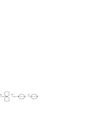
Figure 1: Fig. 1. Two-loop diagrams for the distribution function $F$, corresponding to the terms of Eq. (15). Solid lines denote the diffusons.

3. Perturbation theory. Expanding the Keldysh (upper-right) block of the matrix $Q$ in terms of the diffusons $d$ with the help of Eqs. (7)–(10) one obtains the perturbative series:

$$F=F^{(0)}-\frac{\langle d\rangle}{2}-\frac{\langle F^{(0)}d^{\dagger}d+dd^{\dagger}F^{(0)}\rangle}{4}+\frac{\langle dd^{\dagger}d\rangle}{8}+\dots$$ (14)

The two-loop correction to the distribution function is given by three pairings:

$$\delta F=\frac{\langle d\,S^{(5)}\rangle_{0}}{2}-\frac{\langle d\,S^{(4)}S^{(3)}\rangle_{0}}{2}+\frac{\langle dd^{\dagger}d\,S^{(3)}\rangle_{0}}{8},$$ (15)

shown diagrammatically in Fig. 1. The other possible pairings vanish due to causality of the theory. In Eq. (15), the vertices $S^{(m)}$ come from expansion of the action (4) to the order $W^{m}$. In the rational parametrization (9) they are given by the following expressions:

$$S^{(3)}=\frac{\pi\Gamma}{2\Delta}\int\varphi_{12}\varphi_{34}F_{12}^{(0)}d^{*}_{32}d_{34}d^{*}_{14},$$ (16)

$$S^{(5)}=\frac{\pi\Gamma}{8\Delta}\int\varphi_{12}(\varphi_{34}+\varphi_{56})F_{12}^{(0)}d^{*}_{23}d_{43}d^{*}_{45}d_{65}d^{*}_{61}+\dots,$$ (17)

$$S^{(4)}=-\frac{\pi}{8\Delta}\int(\partial_{5}+\partial_{6})d_{56}d^{*}_{76}d_{78}d^{*}_{58}\\ -\frac{\pi\Gamma}{16\Delta}\int\bigl{(}\varphi_{56}^{2}+\varphi_{58}^{2}+\varphi_{67}^{2}+\varphi_{78}^{2}\\ {}-\varphi_{57}^{2}-\varphi_{68}^{2}\bigr{)}\,d_{56}d^{*}_{76}d_{78}d^{*}_{58}+\dots$$ (18)

The the terms not included in Eqs. (17) and (18) do not contribute to the pairings shown in Fig. 1. In writing Eqs. (16)–(18) we used the concise notations $F_{ij}\equiv F_{t_{i}t_{j}}$, $d_{ij}\equiv d_{t_{i}t_{j}}$, and $\varphi_{ij}\equiv\varphi(t_{i})-\varphi(t_{j})$, with integration being performed over all time arguments involved.

The diagrams (a) and (b) shown in Fig. 1 contain a loose diffuson [2] which couple $d$ to the rest of the diagram. As a result, the corresponding correction to the distribution function $F_{t+\eta/2,t-\eta/2}$ can be written as

$$\delta F_{t+\eta/2,t-\eta/2}^{(ab)}\\ {}=\int dt^{\prime}dt^{\prime\prime}\,\cD_{\eta}(t,t^{\prime})\,\Xi(t^{\prime},t^{\prime\prime},\eta)\,F_{t^{\prime\prime}+\eta/2,t^{\prime\prime}-\eta/2},$$ (19)

where $t^{\prime}$ is the “center of mass” time at the right end of the loose diffuson, and $\Xi(t^{\prime},t^{\prime\prime},\eta)$ is a complicated expression denoting the rest of the diagram. The corresponding correction to the energy absorption rate given by Eq. (13) simplifies to

$$\delta W^{(ab)}(t)=-\frac{1}{\Delta}\lim_{\eta\to 0}\frac{\partial}{\partial\eta}\frac{1}{\eta}\int dt^{\prime\prime}\,\Xi(t,t^{\prime\prime},\eta),$$ (20)

where we employed Eq. (12) and used the asymptotics $F_{t_{+}t_{-}}\sim 1/(i\pi\eta)$ at $\eta\to 0$.

Contrary, the diagram (c) in Fig. 1 does not contain a loose diffuson and cannot be represented in the form (20) with already taken derivative with respect to the external time $t$.

Finally, it is worth mentioning that the diagram (a) is completely canceled against the part of the diagram (b) which contains the time derivative originating from the first term in Eq. (18).

As a result of straightforward but rather lengthy calculation one ends up with the general expression for the two-loop correction to the Kubo dissipation rate (2) valid for an arbitrary $\varphi(t)$:

$$\delta W(t)={} \frac{\Gamma\Delta}{2\pi^{2}}\lim_{\eta\to 0}\frac{\partial}{\partial\eta}\frac{1}{\eta}\int_{0}^{\infty}dx\,dy\,dz\,$$

$$\!{}\times\left(\frac{\partial}{\partial t}-2\Gamma\varphi_{56}\,\varphi_{78}\right)\varphi_{12}\varphi_{34}$$

$$\!{}\times\cD_{\eta+x+y}\left(t-\frac{x}{2}-\frac{y}{2},\,t-\frac{x}{2}-\frac{y}{2}-z\right)$$

$$\!{}\times\cD_{\eta-x-z}\left(t-\frac{x}{2}-\frac{z}{2},\,t-\frac{x}{2}-\frac{z}{2}-y\right)$$

$$\!{}\times\cD_{\eta+y-z}\left(t-\frac{y}{2}-\frac{z}{2},\,t-\frac{y}{2}-\frac{z}{2}-x\right),$$ (21)

where $t_{1,2}=t_{\pm}-x-y-z$, $t_{3}=t_{+}-z$, $t_{4}=t_{-}-y$, $t_{5}=t_{+}-x-z$, $t_{6,7}=t_{\mp}$, and $t_{8}=t_{-}-x-y$. In Eq. (21) the term with $\partial/\partial t$ describes the contribution of the diagram (c) while the rest is the contribution of the diagrams (a) and (b). Thought the derivatives with respect to $\eta$ and $t$ can be easily calculated with the help of Eq. (12) we leave them unevaluated in order to keep the simplest form of the expression.

4. Linear case. We start the analysis of the general formula (21) with the case of a linear bias $\varphi(t)=vt$. Then the dynamic diffuson (12) is given by $\cD_{\eta}(t_{1},t_{2})=\theta(t_{1}-t_{2})\exp\{-\Omega^{3}\eta^{2}(t_{1}-t_{2})\}$ where $\Omega=(\Gamma v^{2})^{1/3}$ is the dephasing rate due to the time-dependent perturbation [3]. Since the diffuson $\cD_{\eta}(t_{1},t_{2})$ depends only on $t_{1}-t_{2}$, the integrand in Eq. (21) does not depend on $t$ and the corresponding time derivative describing the contribution of the diagram (c) vanishes.

The product of three diffusons in Eq. (21) is an even function of $\eta$, hence $\eta$-dependence should be taken into account only in the terms $\varphi_{ij}$. The resulting expression becomes

$$\delta W=\frac{\Omega^{6}\Delta}{\pi^{2}}\int_{0}^{\infty}dx\,dy\,dz\>(-x^{2}+5xy)\\ {}\times\exp\left\{-\Omega^{3}(x+y)(y+z)(z+x)\right\},$$ (22)

where we employed the symmetry between the integration variables to simplify the final expression.

The integrals in Eq. (22) are given by

$$\int_{0}^{\infty}dx\,dy\,dz\genfrac{[}{]}{0.0pt}{}{x^{2}}{xy}e^{-(x+y)(y+z)(z+x)}=\genfrac{[}{]}{0.0pt}{}{5}{1}\times\frac{\Gamma^{2}(1/3)}{48},$$ (23)

leading to a surprising cancelation of the two-loop quantum correction in the unitary case mentioned in Ref. [3].

It is also instructive to consider the case of the linear perturbation switched on at $t=0$: $\varphi(t)=\theta(t)\,vt$. Here the term with $\partial/\partial t$ in Eq. (21) is generally nonzero but it is small in the most interesting limit $\Omega t\gg 1$. The time-dependent $\delta W(t)$ is then given by Eq. (22) where the region of integration is now bounded from above by the condition $x+y+z<t$. The correction to the total absorbed energy becomes

$$\delta E(t)=\frac{\Omega^{6}\Delta}{\pi^{2}}\int_{0}^{\infty}dx\,dy\,dz\>\min(x+y+z,t)\\ {}\times(-x^{2}+5xy)\,e^{-\Omega^{3}(x+y)(y+z)(z+x)}$$ (24)

The integrals with $x^{2}y$ and $xyz$ converge while the integral with $x^{3}$ diverges logarithmically. Therefore, at $\Omega t\gg 1$

$$\delta E(t)\simeq-\frac{\Delta}{\pi^{2}}\ln(\Omega t).$$ (25)

Thus, the two-loop quantum correction, though vanishing for a linear perturbation, leads to a long-time memory effects near the points of discontinuity of $\partial\varphi/\partial t$.

5. Periodic case. Now we turn to the case of periodic perturbations switched on at $t=0$. To simplify calculations we will consider first the simplest example of a monochromatic perturbation, $\varphi(t)=\theta(t)\sin\omega t$. Then the dynamic diffuson (12) acquires the form:

$$D_{\eta}(t,t^{\prime})=\theta(t-t^{\prime})\exp\biggl{\{}-2\Gamma\sin^{2}\frac{\omega\eta}{2}\\ \times\Bigl{[}t-t^{\prime}+\frac{\sin\omega(t-t^{\prime})}{\omega}\cos\omega(t+t^{\prime})\Bigr{]}\biggr{\}}.$$ (26)

It is convenient to calculate the two contributions to Eq. (21), $\delta W^{(ab)}(t)$ and $\delta W^{(c)}(t)$, separately. Making use of Eq. (26) we get:

$$\delta W^{(ab)}(t)=-\frac{2\Gamma^{2}\Delta\omega^{2}}{\pi^{2}}\int_{0}^{x+y+z<t}\!dx\,dy\,dz\;\sC\,\sS\,\sD,$$ (27)

where

$$\sC=\cos\omega(t-x-y-z)\cos\omega\left(t-\frac{x}{2}-\frac{y}{2}\right)\\ {}\times\cos\omega\left(t-\frac{x}{2}-\frac{z}{2}\right)\cos\omega\left(t-\frac{y}{2}-\frac{z}{2}\right),$$ (28)

$$\sS=3\sin^{2}\frac{\vartheta_{x}}{2}-\sin^{2}\frac{\vartheta_{y}}{2}-\sin^{2}\frac{\vartheta_{z}}{2}-4\Gamma\sin\frac{\vartheta_{x}}{2}\\ {}\times\sin\frac{\vartheta_{y}}{2}\sin\frac{\vartheta_{z}}{2}\left(x\sin\vartheta_{x}+y\sin\vartheta_{y}+z\sin\vartheta_{z}\right),$$ (29)

$\sD$ is the product of three diffusons in Eq. (21) evaluated at $\eta=0$, and we introduced $\vartheta_{x}=y-z$, $\vartheta_{y}=-x-z$, and $\vartheta_{z}=x+y$.

The long-time behavior of Eq. (27) is determined by the vicinities of the no-dephasing points [10] where each of the three diffusons entering $\sD$ is equal to 1. An analogous situation arises in the calculation of the one-loop quantum correction for the periodically driven orthogonal matrices [4], which is dominated by the no-dephasing points of a single dynamic cooperon. In the present case, the no-dephasing points are given by $(x,y,z)=(x,2\pi m/\omega-x,2\pi n/\omega-x)$ with arbitrary $x$ and integer $m$ and $n$.

In the limit $t\gg(\omega^{-1}$, $\Gamma^{-1})$ the no-dephasing points with different $m$ and $n$ do not overlap and the triple integral in Eq. (27) can be evaluated as

$$\int dx\,dy\,dz\longrightarrow\int dx\sum_{mn}\int d\delta y\,d\delta z,$$ (30)

where we introduced $y=2\pi m/\omega-x+\delta y$ and $z=2\pi n/\omega-x+\delta z$. At the no-dephasing point the factor $\sC$ is nonzero whereas the factor $\sS$ vanishes and should be expanded in the deviations $\delta y$ and $\delta z$:

$$\sC=\cos^{2}\omega t\,\cos^{2}\omega(t+x),$$ (31)

$$\sS=\frac{\omega^{2}}{4}\left(3(\delta y-\delta z)^{2}-\delta z^{2}-\delta y^{2}\right)\\ +\frac{\Gamma\omega^{4}}{2}\delta y\delta z(\delta y-\delta z)\left[(x+z)\delta y-(x+y)\delta z\right].$$ (32)

Though the last term of Eq. (32) is proportional to the fourth power of $\delta y$ and $\delta z$, their smallness is compensated by an extra factor $x,y,z\sim t$. In the limit $t\gg(\omega^{-1}$, $\Gamma^{-1})$ we can integrate near the no-dephasing points in the Gaussian approximation retaining only quadratic in the deviations terms in $\ln\sD$:

$$\sD=\exp\left\{-\frac{\Gamma\omega^{2}}{2}\left[x(\delta y-\delta z)^{2}+y\delta z^{2}+z\delta y^{2}\right]\right\}.$$ (33)

The weight (33) determines the correlators:

$$M\equiv\begin{pmatrix}\langle\delta y\delta y\rangle&\langle\delta y\delta z\rangle\\ \langle\delta y\delta z\rangle&\langle\delta z\delta z\rangle\end{pmatrix}\\ =\frac{1}{\Gamma\omega^{2}}\frac{1}{xy+yz+zx}\begin{pmatrix}x+y&x\\ x&x+z\end{pmatrix}.$$ (34)

Substituting Eqs. (30)–(34) into Eq. (27) and integrating over $\delta y$ and $\delta z$ one gets

$$\delta W^{(ab)}(t)=-\frac{\Gamma^{2}\Delta\omega^{2}}{\pi^{2}}\cos^{2}\omega t\\ {}\times\int dx\sum_{mn}2\pi\sqrt{\det M}\,\langle\sS\rangle,$$ (35)

where we replaced $\cos^{2}\omega(t+x)$ by its average value 1/2. The average $\langle\sS\rangle$ is calculated with the help of the Wick’s theorem using the pair correlators (34):

$$\langle\sS\rangle=\frac{3xyz}{2\Gamma(xy+yz+zx)^{2}}.$$ (36)

Finally, since the summand in Eq. (35) is a smooth function of $m$ and $n$ it is possible to pass from summation over $m$ and $n$ back to integration over $y$ and $z$:

$$\sum_{mn}\longrightarrow\left(\frac{\omega}{2\pi}\right)^{2}\int dy\,dz.$$ (37)

As a result we obtain

$$\delta W^{(ab)}(t)=-\frac{3\Delta\omega^{2}}{4\pi^{3}}\cos^{2}\omega t\\ {}\times\int_{0}^{x+y+z<t}\frac{xyz\,dx\,dy\,dz}{(xy+yz+zx)^{5/2}}.$$ (38)

This integral is equal to $(2\pi/27)t$ and we get

$$\delta W^{(ab)}(t)=-\frac{\Delta\omega^{2}t}{18\pi^{2}}\cos^{2}\omega t.$$ (39)

The contribution of the diagram (c), $\delta W^{(c)}$, can be calculated analogously. Due to the same structure of the diffusons, its no-dephasing points coincide with the no-dephasing points for $\delta W^{(ab)}$. Instead of Eq. (35) one has now:

$$\delta W^{(c)}(t)=\frac{\Gamma\Delta\omega^{2}}{4\pi^{2}}\frac{\partial}{\partial t}\int dx\sum_{mn}2\pi\sqrt{\det M}\,\langle\sS^{\prime}\rangle,$$ (40)

where

$$\langle\sS^{\prime}\rangle=1-\Gamma\omega^{2}\left<(\delta y-\delta z)\left[(x+z)\delta y-(x+y)\delta z\right]\right>\\ =-\frac{yz}{xy+yz+zx}.$$ (41)

Passing from summation to integration according to Eq. (37) and utilizing the symmetry properties of the integrand we obtain:

$$\delta W^{(c)}(t)=-\frac{\Delta\omega^{2}}{24\pi^{3}}\frac{\partial}{\partial t}\int_{0}^{x+y+z<t}\frac{dx\,dy\,dz}{\sqrt{xy+yz+zx}}.$$ (42)

The integral is equal to $(\pi/6)t^{2}$ yielding

$$\delta W^{(c)}(t)=-\frac{\Delta\omega^{2}t}{72\pi^{2}}.$$ (43)

Note a peculiar property of Eqs. (39) and (43): $\delta W^{(ab)}(t)\propto t(d\varphi/dt)^{2}$ and vanishes at the turning points of the perturbation, whereas $\delta W^{(c)}(t)$ is always positive, even when $d\varphi/dt=0$. This means that they describe different mechanisms of absorption, with different memories on the past.

Combining Eqs. (39) and (43) we get the total two-loop correction to the quasiclassical absorption rate in the harmonic case:

$$\delta W(t)=-\frac{\Delta\omega^{2}t}{72\pi^{2}}\left[4\cos^{2}\omega t+1\right],$$ (44)

valid at $t\gg(\omega^{-1}$, $\Gamma^{-1})$.

The time-averaged correction grows linearly with the duration of the perturbation:

$$\overline{\delta W(t)}=-\frac{\Delta\omega^{2}t}{24\pi^{2}}.$$ (45)

Remarkably, Eq. (45) holds not only for a harmonic perturbation but for an arbitrary periodic perturbation with the period $2\pi/\omega$. Formally this follows from the fact that the level sensitivity $\Gamma$ to the external perturbation drops from Eq. (45). Then, according to Eq. (37), the factor $\omega^{2}$ in Eq. (45) measures the inverse time separation between the no-dephasing points which is the same for all periodic perturbations of a given period.

6. Dynamic vs. Anderson localization. It is useful to compare the two-loop result (45) for a harmonic perturbation with the analogous one-loop expression for the GOE obtained in Ref. [4]:

$$\frac{\overline{\delta W(t)}}{\overline{W_{0}}}=-\begin{cases}\displaystyle\sqrt{\frac{t}{t_{*}}},&\text{GOE},\\[8.0pt] \displaystyle\frac{\pi t}{24t_{*}},&\text{GUE},\end{cases}$$ (46)

where $\overline{W_{0}}=\pi\Gamma\omega^{2}/2\Delta$ is the period-averaged absorption rate, and $t_{*}=\pi^{3}\Gamma/2\Delta^{2}$ is the localization time.

In Ref. [4] we pointed out that the weak dynamic localization correction to the energy absorption rate of a periodically driven GOE has the same square-root behavior as the weak Anderson localization correction to the conductivity of a quasi-one-dimensional (1D) disordered wire. Now we see that the same is true for the case of the GUE as well: in both cases the correction is linear in time and dephasing time, respectively. Therefore it is tempting to suggest that this analogy is not a coincidence but has its roots in equivalence between the dynamic localization for the RMT driven by a harmonic perturbation and 1D Anderson localization.

Such an equivalence is known for the case of kicked quantum rotor (KQR): in the long time limit, the KQR problem can be mapped [11] onto the 1D $\sigma$-model. On the other hand, the problems of the $\delta$-kicked KQR and of the periodically driven RMT are, to some extent, complementary. Both of them can be mapped on a tight-binding 1D model, but with very different structure of couplings between the sites and auxiliary orbitals [4]. In particular, the “kicked RMT” model with $\varphi(t)$ being a periodic $\delta$-function does not exhibit dynamic localization whatsoever [4].

In order to check the assumption about the equivalence of the driven RMT to the quasi-1D disordered wire we use the simple relationship between the time-dependent energy absorption rate $W(t)$ in the dynamic problem and the frequency-dependent diffusion coefficient $D(\omega)$ in the Anderson model [12]:

$$\frac{W(t)}{W_{0}}=\int_{-\infty}^{+\infty}\frac{d\omega}{2\pi}\frac{e^{-i\omega t}}{-i\omega+0}\,\frac{D(\omega)}{D_{0}},$$ (47)

where $W_{0}$ and $D_{0}$ are the classical period-averaged absorption rate and diffusion coefficient. $D(\omega)$ is known from the theory of weak Anderson localization:

$$\frac{\delta{D}(\omega)}{D_{0}}=\begin{cases}\displaystyle-\frac{1}{\sqrt{-i\omega t_{\text{loc}}}},&\text{GOE},\\[8.0pt] \displaystyle\frac{1}{6i\omega t_{\text{loc}}},&\text{GUE}.\end{cases}$$ (48)

Here $t_{\text{loc}}=(2\pi\nu_{1})^{2}D_{0}$, and $\nu_{1}$ is the 1D density of states. Then Eqs. (48), (47) give two expressions similar to Eq. (46) with only one fitting parameter $t_{*}/t_{\rm loc}$. One can easily see that with the choice $t_{*}/t_{\text{loc}}=\pi/4$ both numerical coefficients match exactly.

We believe that there are deep reasons for this coincidence and make a conjecture that the (period-averaged) dynamics of the harmonically-driven RMT at time scales $t\gg(\omega^{-1}$, $\Gamma^{-1})$ is equivalent to the density propagation in a quasi-1D disordered wire. Employing this equivalence, we can easily calculate the energy absorption rate in the regime of well developed dynamic localization at $t\gg t_{*}$ using the Mott-Berezinsky asymptotics of the AC conductivity, $\sigma(\omega)\propto\omega^{2}\ln^{2}(1/\omega)$ [13, 14]. Substituting $D(\omega)\propto\sigma(\omega)$ into Eq. (47) we find that in the localized regime $W(t)$ decays as

$$W(t)\propto\frac{\ln t}{t^{2}},\qquad t\gg t_{*}.$$ (49)

This dependence is not directly related to the spatial dependence of the localized wave functions which is exponential in the Anderson model. It can be seen if one considers the density-density correlator [disorder-averaged product of the retarded and advanced Green’s functions $G^{R}(x,x^{\prime},\epsilon+\omega)G^{A}(x^{\prime},x,\epsilon)$] whose Fourier transform can be conveniently represented as $2\pi\nu_{1}\,A(k,\omega)/(-i\omega)$. According to Gorkov’s criterion of localization [15], $A(k,0)$ is finite and its Fourier transform determines the spatial decay of localized wavefunctions. On the other hand, $D(\omega)$ can be extracted from the density-density correlator as

$$D(\omega)=\frac{i\omega}{2}\frac{\partial^{2}}{\partial k^{2}}A(k,\omega)\Bigr{|}_{k=0},$$ (50)

and, according to our conjecture, should be substituted in Eq. (47) to give the absorption rate. Thus, instead of $A(k,\omega=0)$, usually studied in the Anderson localization problem, $W(t)$ is determined by the $\omega$ dependence of $\partial^{2}A(k,\omega)/\partial k^{2}$ at $k=0$, which to the best of our knowledge evaded investigation in the framework of the quasi-1D nonlinear sigma model.

7. Conclusion. We derived the general expression for the lowest order (two-loop) interference correction to the energy absorption rate of a parametrically-driven GUE. If an external perturbation grows linearly with time the first correction vanishes. For a periodic perturbation the averaged correction $\delta W(t)\propto t$. We make a conjecture that the dynamics of the harmonically-driven RMT at the time scales $t\gg 1/\omega,1/\Gamma$ is equivalent to the 1D Anderson model. Based on this equivalence we predict that in the regime of strong dynamic localization $W(t)\propto\ln(t)/t^{2}$.

M. A. S. acknowledges financial support from the RFBR grant No. 04-02-16998, the Russian Ministry of Science and Russian Academy of Sciences, the Dynasty Foundation, the ICFPM, and thanks the Abdus Salam ICTP for hospitality.

References

[1]
M. G. Vavilov and I. L. Aleiner, Phys. Rev. B
60, R16311 (1999); 64, 085115 (2001);
M. G. Vavilov, I. L. Aleiner, and V. Ambegaokar, Phys. Rev. B
63, 195313 (2001).
[2]
V. I. Yudson, E. Kanzieper, and V. E. Kravtsov, Phys. Rev. B 64,
045310 (2001).
[3]
M. A. Skvortsov, Phys. Rev. B 68, 041306(R) (2003).
[4]
D. M. Basko, M. A. Skvortsov, and V. E. Kravtsov,
Phys. Rev. Lett. 90, 096801 (2003).
[5]
K. B. Efetov, Supersymmetry in Disorder and Chaos (Cambridge
University Press, New York, 1997).
[6]
V. E. Kravtsov, cond-mat/0312316.
[7]
M. Wilkinson, J. Phys. A: Math. Gen. 21, 4021 (1988).
[8]
B. D. Simons and B. L. Altshuler,
Phys. Rev. B 48, 5422 (1993).
[9]
G. Casati, B. V. Chirikov, J. Ford, and F. M. Izrailev,
in Stochastic Behaviour in Classical
and Quantum Hamiltonian Systems, ed. by G. Casati and J. Ford,
Lecture Notes in Physics, vol. 93 (Springer, Berlin, 1979).
[10]
X.-B. Wang and V. E. Kravtsov, Phys. Rev. B 64, 033313 (2001).
[11]
A. Altland and M. R. Zirnbauer, Phys. Rev. Lett. 77, 4536 (1996).
[12]
A. Altland, Phys. Rev. Lett. 71, 69 (1993);
C. Tian, A. Kamenev, and A. Larkin, cond-mat/0403482.
Although in these works Eq. (48) was applied to the KQR,
its validity is not restricted just by the KQR case.
[13]
N. F. Mott, Phylos. Mag. 17, 1259 (1968).
[14]
V. L. Berezinskii,
Zh. Eksp. Teor. Fiz. 65, 1251 (1973)
[Sov. Phys. JETP 38, 620 (1974)].
[15]
V. L. Berezinskii and L. P. Gor’kov,
Zh. Eksp. Teor. Fiz. 77, 2498 (1979) [Sov. Phys. JETP 50, 1209 (1979)].