Optical study on doped polyaniline composite films

Abstract

Localization driven by disorder has a strong influence on the conducting property of conducting polymer. A class of authors hold the opinion that disorder in the material is homogeneous and conducting polymer is disordered metal close to Anderson-Mott Metal-Insulator transition, while others treat the disorder as inhomogeneous and have the conclusion that conducting polymer is a composite of ordered metallic regions and disordered insulating regions. The morphology of conducting polymers is an important factor that have influence on the type and extent of disorder. Different protonic acids used as dopants and moisture have affection on polymer chain arrangement and interchain interactions. A PANI-CSA film, two PANI-CSA/PANI-DBSA composite films with different dopants ratio, and one of the composite films with different moisture content are studied. Absolute reflectivity measurements are performed on the films. Optical conductivity and the real part of dielectric function are calculated by Kramers-Kronig(KK) relations. $\sigma_{1}(\omega)$ and $\varepsilon_{1}(\omega)$ derivate from simple Drude model in low frequency range and tendencies of the three sample are different and non-monotonic. The Localization Modified Drude model(LMD) in the framework of Anderson-Mott theory can not give a good fit to the experimental data. By introducing a distribution of relaxation time into LMD, reasonable fits for all three samples are obtained. This result supports the inhomogeneous picture.

I Introduction

Doped conducting polymers are widely studied since 1980s. Although the room temperature DC conductivity of these material has reached that of normal metals, and some other metallic features like finite zero temperature conductivity, negative dielectric constant are observed, the quasi-1D nature of polymer chains indicates that its conducting mechanism is different from conventional metals. Because conducting polymer samples are piled up by a large number of polymer chains, the morphology of sample has important influence on its conductivity. Disorder is usually discussed and remains controversial about whether it is homogeneous or inhomogeneous in conducting polymers.Kohlman and Epstein (1998); Menon et al. (1998)

It is known that disorder is determined by several factors, mainly including dopants used, sample preparing procedure and later treatments. Different protonic acids used as dopants have different molecular sizes, weights and electronegativity, and thus will affect polymer chain arrangement and interchain interactions. Compared with other factors, dopants can be quantitatively controlled more easily. In this study, dopants used are camphor sulfonic acid(CSA) and dodecylbenzene sulphonic acid(DBSA). A PANI-CSA film and two PANI-CSA/PANI-DBSA composite films with different dopants ratio are studied, also one of the composite films with different moisture content. Optical reflectivity measurements are performed on the samples. $\rho_{DC}(T)$ provides a basic understanding of conducting properties and are used to identify different transport regimes in the existence of Metal-Insulator Transition (MIT). However, macroscopic T dependence of DC resistivity may not correspond to only one microscopic transport mechanism, and in conducting polymers there may be several charge transfer processes with different time scales coexisting.Prigodin and Epstein (2002) Reflectivity spectra, along with optical conductivity and the real part of dielectric function calculated by KK relations, could probe the response of electron system over a large energy range and different time scales. It is an effective way for the investigation of charge transport mechanism and several intensive studies on reflectivity of conducting polymers exist. Although the reported reflectivity data have similar features, analysis and explanation of optical conductivity and the real part of dielectric function remain controversial, especially in low frequency behaviors. Lee et al. (1993); Kohlman et al. (1997a); Tzamalis et al. (2002); Chapman et al. (1999) We observed different and non-monotonic tendency in low frequency range of the samples and tried to explain the behavior in a unified framework.

II Experiment

Aniline monomer is polymerized in solution in the presense of protonic acid(CSA/DBSA) as dopant, then Ammonium persulfate as oxidant is dissolved in deionized water and slowly added into previously cooled mixture. After all the oxidant is added, the reaction mixture is stirred for 24h. The precipitate is then washed with deionized water, methanol and ethylether separately for several times, and dried at room temperature in a dynamic vacumm for 24h to finally obtain the powder of doped polyaniline. To prepare porous PANI-CSA/PANI-DBSA composite films, preparation of PANI-CSA m-cresol solution and preparation of PANI-DBSA chloroform solution are done separately and then the two solutions with appropriate ratio were mixed and combined with supersonic stirring. Porous films were obtained by casting the blend solution onto a glass plate. After drying at room temperature in air the polyblend was peeled off the glass substrate to form a free-standing film.

The near-normal incidence reflectance spectra were measured by using a Bruker IFS66v/S spectrometer in the frequency range from 40$cm^{-1}$ to 25000$cm^{-1}$. The sample was mounted on an optically black cone in a cold-finger flow cryostat. An in situ overcoating techinque was employed for reflectance measurement, Homes et al. (1993)which could remove the effect caused by non flatness of sample surface. A series of light sources,beam splitters and detectors were used in different frequency ranges.The connections between different regions were excellent because of the identical overlap. The optical conductivity and dielectric constants were calculated by KK relation of the reflectivity data. At low frequency end, Hagen-Rubens relation was used to extrapolate data towards zero as in most literatures. At high frequency end of measurement, $R(\omega)$ was extrapolated using $R\propto\omega^{-2}$ to 300000 $cm^{-1}$, and beyond that a free electron behavior of $R\propto\omega^{-4}$ was used.

III Results and Discussion

It is known from reported data that PANI-CSA is more conductive than PANI-DBSA Lu et al. (2002); Long et al. (2003), because of its smaller counterion size and therefore stronger interchain interactions. We label the pure PANI-CSA film, the 15% PANI-CSA/85%PANI-DBSA blend, the 5%PANI-CSA/95% PANI-DBSA blend sample A, B, C, respectively, in the later part of this paper. Temperature-dependent DC conductivity measurements show that $\rho_{DC}|_{C}>\rho_{DC}|_{B}>\rho_{DC}|_{A}$, as in Fig.1. The activation energy $W=d(ln\sigma)/d(lnT)$ is used as a more effective criteria in the existence of a MIT Menon et al. (1993). The slope of the plot is positive, negative and constant at low temperature for sample in the metallic, the insulating and the critical regime, respectively. Inset of Fig. 1 is the W vs.T plot. Sample A has a positive slope at low temperature, confirming that there are delocalized states at the Fermi level as $T\rightarrow 0$ and this sample is in the metallic region of MIT. The slope of sample B and C has weak T dependence indicating they are near the critical regime of MIT.

Figure 1: $\rho_{DC}$ of sample A, B and C, from 8-300K. B dried is the DC resistivity of sample B measured after storing in ambient air for several months, down to 2K. There is a tiny elevation in value.Inset is the activation energy $W=d(ln\sigma)/d(lnT)$ for the three samples. $\rho_{DC}(T)$ of all samples are first fitted by six order polynomial and later calculation is based on the fitting formula, the plot range is 8-300K

Part (a) of Fig.2 is the measured reflectivity data. At the low frequency end, the subsequence of the reflectivity magnitude of the three samples is the same as that of their $\rho_{DC}(RoomT)$. Part (b) is the real part of $\sigma(\omega)=\sigma_{1}(\omega)+\imath\sigma_{2}(\omega)$, which is obtained through KK relations, with similar features of reported data of a series of protonic acid doped PANI and Ppy samples Lee et al. (1993); Tzamalis et al. (2002, 2001); Lee et al. (1995a, b); Chapman et al. (1999); Lee and Heeger (2003). The peak around $19000cm^{-1}$ corresponds to $\pi-\pi^{\ast}$ interband transition. There are a series of sharp peaks between 1000-1800 $cm^{-1}$, which are accounted for as phonon features, the peak position corresponding to certain bond vibration modes was given in literature elsewhere Lu et al. (2002). Between 1000 and 10000 $cm^{-1}$, $\sigma_{1}$ has a Drude type behavior. Below 1000$cm^{-1}$, disregarding the phonon features, $\sigma_{1}$ deviates from Drude model that it decreases with decreasing frequency. This deviation is generally considered as the effect of localization of electron wave functions. At the far IR region, $\sigma_{1}(\omega)$ of the three samples have different variation tendency. $\sigma_{1}(\omega)$ of sample A and C begin to increase below about $100cm^{-1}$, while $\sigma_{1}(\omega)$ of sample B remains decreasing till the low frequency edge of our measurement. This character is more obvious in linear axes. Additionally, $\sigma_{1}(\omega)|_{B}$ is larger than $\sigma_{1}(\omega)|_{A}$ in $100-1000cm^{-1}$ range. This behavior of optical conductivity is not consistent with $\rho_{DC}(T)$, which scales with the ratio of dopping protonic acids used, and suggests that the charge transport process in conducting polymer cannot be fully manifested in DC resistivity.

Figure 2: Part (a) is the reflectivity data for all samples, part (b) is the real part of $\sigma(\omega)=\sigma_{1}(\omega)+\imath\sigma_{2}(\omega)$ of sample A, B and C, note the difference tendency in low frequency range

There is large contradiction in the reported $\varepsilon_{1}(\omega)$ of $\varepsilon(\omega)=\varepsilon_{1}(\omega)+\imath\varepsilon_{2}(\omega)$ derived from KK. Some authors reported large negative value of $\varepsilon_{1}(\omega)$ in the far infrared range Kohlman et al. (1995, 1996); Kohlman et al. (1997b), while others reported positive $\varepsilon_{1}(\omega)$ in the same range Lee et al. (1993, 1995b). Due to suspicion to $\varepsilon_{1}(\omega)$ near the low measurement edge obtained through KK, all the authors had made effort to ensure the effectiveness of data. Besides affirming the reflectivity measurements, the direct dielectric measurements are used as boundary condition Joo et al. (1994); Martens et al. (2001a, b); Lee and Heeger (2003); Romijin et al. (2003). The consistency between $\sigma_{1}(\omega)$ and $\varepsilon_{1}(\omega)$ is also discussed, the results of KK should stand by causality lawKittel (1976). Fig.3 is our result of $\varepsilon_{1}(\omega)$. Features in high frequency range are similar with reported data. In far IR range, $\varepsilon_{1}(\omega)|_{A}$ has a turnover at approximately 300 $cm^{-1}$ and a crossover at 106 $cm^{-1}$, and then becomes negative; $\varepsilon_{1}(\omega)|_{C}$ has a turnover at about 100 $cm^{-1}$ and decrease to nearly zero at 50 $cm^{-1}$; $\varepsilon_{1}(\omega)|_{B}$ has no turnovers and remains increasing with decreasing frequency. Here, the low frequency behavior shows non-monotonic change again. It is noted that changes in $\sigma_{1}(\omega)$ is correlated with changes in $\varepsilon_{1}(\omega)$. Increasing at low frequency in $\sigma_{1}(\omega)$ is a Drude type behavior, corresponding to negative $\varepsilon_{1}(\omega)$ values because the polarization of electron systems is out of phase with the external field. Considering the background $\varepsilon_{\infty}$of conducting polymers, $\varepsilon_{1}(\omega)$ should decrease with decreasing frequency at low energy and become negative after a crossover. Inset of Fig. 3 is the $\varepsilon_{1}(\omega)$ vs. $1/\omega^{2}$ plot for sample A and C in the low frequency range, confirming the existence of Drude type behavior. We hence hold that our $\sigma_{1}(\omega)$ and $\varepsilon_{1}(\omega)$ data are reasonable.

Figure 3: The real part of dielectric function $\varepsilon(\omega)=\varepsilon_{1}(\omega)+\imath\varepsilon_{2}(\omega)$, $\varepsilon_{1}$ of sample A and C have a turnover and $\varepsilon_{1}$ of A becomes negative below 100$cm^{-1}$. Inset is the $\varepsilon_{1}$ vs.$1/\omega^{2}$ plot for sample A and C in low frequency range. Note that a linear relationship between $\varepsilon_{1}$ and $1/\omega^{2}$ is Drude type response: $\varepsilon_{\omega}=\varepsilon_{\infty}-\frac{\omega^{2}_{p1}}{\omega^{2}}$. The fitting $\omega_{p1}$ is 384 $cm^{-1}$, 225 $cm^{-1}$ for sample A and C, respectively.

Hopping behavior observed in $\sigma_{DC}(T)$Zuppiroli et al. (1994) and deviation from Drude Model in $\sigma_{1}(\omega)$ and $\varepsilon_{1}(\omega)$ suggests that localization must be considered in conducting polymers. Because the mesoscopic morphology of samples are tangly built up network of polymer chains, the main source of localization should be structural disorder. Whether the disorder is homogenous or inhomogenous is still in debate. Although our $\sigma_{1}(\omega)$ and $\varepsilon_{1}(\omega)$ data have give us some hints of inhomogeneity, we still begin our fit using homogenous model because of calculation simplicity. In the homogenous disorder model, Localization Modified Drude model(LMD) in the framework of Anderson-Mott localization theory is widely used to fit $\sigma_{1}(\omega)$ and $\varepsilon_{1}(\omega)$ Menon et al. (1998):

$$\sigma_{LMD}(\omega)=\frac{\omega_{p}^{2}\tau}{4\pi(1+\omega^{2}\tau^{2})}$$

$$\times[1-\frac{C}{(k_{F}v_{F})^{2}\tau^{2}}+\frac{C}{(k_{F}v_{F})^{2}\tau^{3/2}}(3\omega)^{1/2}]$$ (1a)

$$\varepsilon_{LMD}(\omega)=\varepsilon_{\infty}+\frac{\omega_{p}^{2}\tau^{2}}{1+\omega^{2}\tau^{2}}$$

$$\times[\frac{C}{(k_{F}v_{F})^{2}\tau^{2}}(\sqrt{\frac{3}{\omega\tau}}-(\sqrt{6}-1))-1]$$ (1b)

where $\omega_{p}$ is the plasma frequency, $k_{F}$ is the Fermi wavevector, $v_{F}$ is the Fermi velocity, $\tau$ is the relaxation time and $\varepsilon_{\infty}$ is the high energy dielectric constant, C is a universal constant($\sim 1$). Fig. 4 is the plot of $\sigma_{1}(\omega)|_{A}$and its LMD fit, range from $50--1000cm^{-1}$. Disregarding the phonon features, the LMD model gives a good fit to the experimental data except in low frequency range. The fitting parameters and deduced values for samples are in Table 1.

Figure 4: The LMD model fit of sample A, range from 50-8000 $cm^{-1}$. Inset is comparasion of $\varepsilon_{1}(\omega)$ given by the LMD model using same parameters of $\sigma_{1}(\omega)$ fit and experimental data. For sample A and C, the fitting curve and experimental data have opposite behaviors in low frequency range

Table 1: Fitting parameters of the LMD model, $\sigma_{1}(0)$is the calculated zero frequency optical conductivity. Note that they are not in good accordance with room temperature $\sigma_{DC}$, $k_{F}\lambda$ is calculated by $k_{F}v_{F}\times\tau$

	$\omega_{p}$	$1/\tau$	$\frac{C}{(k_{F}v_{F})^{2}}$	$\sigma_{1}(0)$	$\sigma_{DC}(RT)$	$k_{F}\lambda$
sample	$(cm^{-1})$	$(cm^{-1})$	$(s^{2})$	$(S/cm)$	$(S/cm)$
A	12185	1/0. 00013	$1.31e^{-31}$	233	241	1. 91
B	7976	1/0. 00033	$1.17e^{-30}$	216	174	1. 62
C	6823	1/0. 00028	$1.65e^{-30}$	55	110	1. 16

The order parameter $k_{F}\lambda$ for three samples are all close to the Ioffe-Regel criterion $k_{F}\lambda\sim 1$, indicating that these samples are close to a MIT according with the activation energy $W=d(ln\sigma)/d(lnT)$ plot. The values of $\tau$ have a magnitude of $10^{-15}s$, same as previous studies. However, there are some erratic behaviors in $\sigma_{1}(\omega)$ which could not be satisfactorily explained. Sample A of the largest $\sigma_{DC}(RoomT)$has the shortest relaxation time. Relaxation time is a reflection of the extent of disorder of material. Whether this fact accounts for the non-monotonic variation of $\sigma_{1}(\omega)$ in far IR is not clear . The increasing tendency of $\sigma_{1}(\omega)$ of sample A and C in the low energy end could not be fitted by LMD using these parameters either. Inset of Fig. 4 is the plot of $\varepsilon_{1}(\omega)$ with LMD fit using the same parameters from $\sigma_{1}(\omega)$ fit. It is clear that $\varepsilon_{1}(\omega)$ of LMD could not simulate the decreasing tendency at low frequency of sample A and C. In LMD model, the low frequency $\sigma_{1}(\omega)$ is suppressed due to localization, and $\varepsilon_{1}(\omega)$ becomes positive because disorder scattering reduces relaxation time. Although there is good fit for sample B in both $\sigma_{1}(\omega)$ and $\varepsilon_{1}(\omega)$, the Drude type behavior of sample A and C at low frequency indicates that the LMD model is not fully applicable in present study. Inhomogeneity in samples must be considered.

In an inhomogenous picture, conducting polymers are treated as composite materials containing mesoscopic ordered regions and amorphous regions. In the ordered regions, polymer chains have good spacial alignment and thus good interchain overlaping, Electrons in these regions are delocalized and show metallic behavior. In the disordered regions, quasi-one dimentional localization plays the dominant role because of the quasi-one dimentional nature of a single polymer chain. In this picture, the Drude type response in $\sigma_{1}(\omega)$ and $\varepsilon_{1}(\omega)$ at low far-IR range is explained by a small fractions of delocalized charge carriers with very long relaxation time$\sim 10^{-13}s$, as indicated by a very small plasma frequency in $\varepsilon_{1}(\omega)$, while the most part of carriers are localized. It is clear that movement of electrons within a ordered region, between ordered regions and in disordered regions have different mechanisms and characteristic time scales, so it is difficult to describe the energy dependence of response by uniform formula over a wide frequency range. Considering that the general feature of $\sigma_{1}(\omega)$ at high frequency can be fitted by both a homogeneous model or an inhomogenous modelRomijin et al. (2003), we followed ref.Kohlman and Epstein (1998) using a distribution function of relaxation time $\tau$ to introduce inhomogeneity into the LMD model. $\tau$ of most part of carriers has a magnitude of $10^{-15}$ as Ioffe-Regel criterion $k_{F}\lambda\sim 1$ allowed, while a small fraction of carriers has a long $\tau$ as experimentally observed. $\sigma_{1}(\omega)$ and $\varepsilon_{1}(\omega)$ are given as:

$$\sigma_{inhomo}(\omega) = \int^{\infty}_{0}P(\tau)\sigma_{LMD}(\omega,\tau)d\tau$$ (2a)

$$\varepsilon_{inhomo}(\omega) = \int^{\infty}_{0}P(\tau)\varepsilon_{LMD}(\omega,\tau)d\tau$$ (2b)

$P(\tau$) is the distribution function of relaxation time.

$$P(\tau)=\frac{2\Delta}{\pi}\left[\frac{\tau^{2}}{(\tau^{2}-\tau_{0}^{2})^{2}+\tau^{2}\Delta^{2}}\right]$$ (3)

$\tau_{0}$ is the average relaxation time, $\triangle$ is the expansion of relaxation time. Fig. 5 is the $\sigma_{1}(\omega)$ and $\varepsilon_{1}(\omega)$ fit for sample A, B and C, fitting parameters are in Table 2.

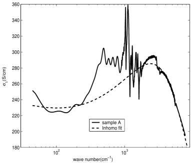
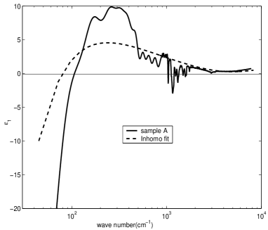
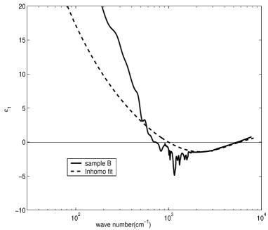
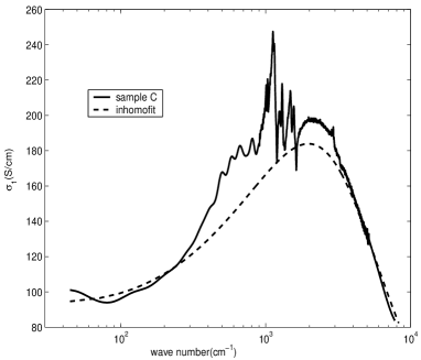
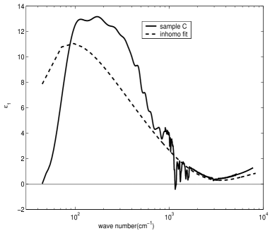
Figure 5: Fits of the LMD model with a distribution of relaxation time. The Drude type behavior of sample A and C in low frequency range are roughly simulated. There is also a qualitatively good fit for sample B.

Table 2: Fitting parameters of the LMD model with a distribution of relaxation time $\tau$, $\Delta$ is the expansion of relaxation time

	$\omega_{p}$	$1/\tau_{0}$	$\frac{C}{(k_{F}v_{F})^{2}}$	$1/\Delta$	$\sigma_{1}(0)$
sample	$(cm^{-1})$	$(cm^{-1})$	$(s^{2})$	($cm^{-1})$	(S/cm)
A	10900	1/0. 00015	$4.50e^{-31}$	1/0. 000017	328
B	7880	1/0. 00031	$1.18e^{-30}$	1/0. 00000027	180
C	6500	1/0. 00027	$2.17e^{-30}$	1/0. 000037	177

Behaviors in low frequency range for the three samples are all qualitatively simulated by including the distribution function of $\tau$. The ratio $\triangle/\tau_{0}$ for sample A and C $\sim 0.1$, while that for sample B $\sim 0.001$. As an estimation, integration of $\tau$ from $0.5\times 10^{2}\tau_{0}$ to $5\times 10^{2}\tau_{0}$ would give the fraction of carrier concentration whose ralaxation time has the magnitude of $10^{-13}s$, the results are 0.001 for sample A and C, and 0.0001 for sample B. Another estimation of the fraction, is to compare the small plasma frequency $\omega_{p1}$ derived from the low frequency $\varepsilon_{\omega}$ vs. $1/\omega^{2}$ plot in fig.3 and the plasma frequency $\omega_{p}$ from LMD fit, as done in ref.Kohlman et al. (1996):

$$\delta=(m^{*}_{1}/m^{*})(\omega_{p1}/\omega_{p})^{2}$$ (4)

The results are 0.00099, 0.0011 for sample A and C, respectively. Although $\omega_{p1}$ derived from such a small frequency range and the assumption that $m^{*}_{1}\sim m^{*}$ are doubtful, we still see that the two estimations give the same results, indicating that there are more carriers with long relaxation time existing in sample A and C, and increasing in $\triangle$ will induce a turnover from positive $\varepsilon_{1}$ to negative.

Although sample B have the largest average $\tau_{0}$, the tiny expansion indicates that $\tau$ of most of its carriers have the scale $10^{-15}$ as Ioffe-Regel criterion predicted, so localization effect is dominant in sample B while sample A and C have a fraction of carriers showing behavior of delocalized electrons.This non-monotonicity results from the difference in the extent of disorder, or, the intensity of intra and interchain interactions, which is not entirely determined by the composition of the samples. The presense of moisture has been observerd to affect the DC conductivity of conducting polymers significantly Kahol et al. (1997), and the moisture influence on sample quality should be manifested in optical data. Reflectivity measurements are performed on two samples which have the same composition as sample B, one is stored in ambient air for over 12 months (B-dried), whose DC resistivity data are show in Fig.1, and the other is also stored but damped with water just before measurements (B-wet). Fig. 6 shows the optical conductivity for sample B, B-dried and B-wet. $\sigma_{1}(\omega)$ of B-dried is lower than B in far-IR range, with the similar tendency, while that of B-wet is larger than B below 100 $cm^{-1}$. It is assumed that removal of water molecules will reduce the structrual order between polymer chains in the metallic regions as well as on chains bridging the metallic regions, in an inhomogeneous picture Pinto et al. (1996), so the increasing in low frequency $\sigma_{1}(omega)$ of B-wet can be interpreted as enhancement of tunneling between metallic regions in low frequency Prigodin and Epstein (2002) due to reduced potential barriers, as water molecules could reduce polarization effects of the counter-anion, hence decrease scattering cross section due to the counter-anions. A fit to B-wet as done in last paragraph gives $\omega_{p}$=8500 $cm^{-1}$, $1/\tau_{0}$=0.00024 $cm^{-1}$, $c/(k_{F}v_{F})^{2}$=5.9$e^{-31}$ $s^{2}$, $1/\Delta$=0.000008 $cm^{-1}$. The ratio $\Delta/\tau_{0}\approx 0.03$, obviously larger than that of B, indicating that in the wet sample the concentration of carriers with a long $\tau$ increases. However, $\sigma_{1}(\omega)$ of B-wet is lower than B in 200-1000 $cm^{-1}$, almost the same as B-dried, its $\varepsilon_{1}(\omega)$ (inset of Fig.6) is lower than B and B-dried but is still positive with two turnovers. This suggests that the increasing in tunneling rate between grains can not compensate the holistic increase of disorder, and according with the conclusion that low frequcy behavior is determined by the competition between coherent and incoherent channels Romijin et al. (2003).

Figure 6: Optical conductivity of sample B and its dried and moistured form, Inset is their $\varepsilon_{1}(\omega)$ plot

IV Conclusion

Absolute reflectivity measurements are performed on one PANI-CSA film, two PANI-CSA/PANI-DBSA composite films, and one of the composite films with different moisture content. Variation of counter-ion composition and moisture content is supposed to modulate polymer chain arrangement and interactions. The charge transport process in conducting polymer cannot be fully manifested in DC resistivity. Optical conductivity and the real part of dielectric function are calculated through Kramers-Kronig relations, the validity of data is discussed. $\sigma_{1}(\omega)$ and $\varepsilon_{1}(\omega)$ derivate from simple Drude model in low frequency range and tendencies of the samples are different and non-monotonic. The localization modified Drude model in the framework of homogeneous disorder cannot explain the behavior of two samples. After considering the inhomogeneity by inducing a distribution function of relaxation time into the LMD model, $\sigma_{1}(\omega)$ and $\varepsilon_{1}(\omega)$ of the samples are all qualitatively well fitted and explained. This result supports the picture that disorder in the samples are inhomogeneous and the samples are consisted of ordered metallic regions and disordered regions.