Well-defined quasiparticles in interacting metallic grains

Abstract

We analyze spectral functions of mesoscopic systems with large dimensionless conductance, which can be described by a universal Hamiltonian. We show that an important class of spectral functions are dominated by one single state only, which implies the existence of well-defined (i.e. infinite-lifetime) quasiparticles. Furthermore, the dominance of a single state enables us to calculate zero-temperature spectral functions with high accuracy using the density-matrix renormalization group. We illustrate the use of this method by calculating the tunneling density of states of metallic grains and the magnetic response of mesoscopic rings.

The pairing Hamiltonian of Bardeen, Cooper and Schrieffer (BCS) is established as the paradigmatic framework for describing superconductivity Cooper et al. (1957); Tinkham (1996). The BCS solution is, however, an approximate one, valid (and exceedingly successful) only as long as the mean level spacing $d$ is much smaller than the superconducting band gap $\Delta_{\mathrm{BCS}}$ von Delft and Ralph (2001); Schechter et al. (2001). One of the main features of the BCS solution is the description of the excitation spectrum by well-defined (i.e. infinite-lifetime) Bogoliubov quasiparticles, responsible for many of the features of the superconducting state.

In this Letter, we address the question whether this quasiparticle picture prevails in the entire regime of parameters – including the case that the samples are so small or so weakly interacting that the BCS solution is inapplicable – by analyzing spectral functions. For example, the spectral function corresponding to the (noninteracting) particle creation operator $c^{\dagger}_{k\sigma}$ is given, within the BCS solution, by a sharp line in $k$-$\omega$-space; this reflects the infinite lifetime of the quasiparticles. For an interacting system, this is a very peculiar property, since the interactions usually shift a significant portion of the spectral weight to a background of excitations, responsible for the finite lifetime of the quasiparticles. Here we show that the unusual property of finding well-defined quasiparticles persists to a very good approximation over the entire parameter range of the pairing Hamiltonian, and is not merely a property of the mean field approximation in the BCS regime. We also give a condition for more general spectral functions to show analogous behaviour.

Of central importance is that this result is relevant not only in the context of mesoscopic superconductivity, but more generally for disordered systems with large dimensionless conductance $g$ (defined as the ratio between the Thouless energy and the mean level spacing $d$). This is because to lowest order in $g^{-1}$, the electron-electron interactions can be described by a remarkably simple universal Hamiltonian (UH) Kurland et al. (2000); Aleiner et al. (2002), which has, besides the kinetic energy term $H^{0}=\sum_{i\sigma}\epsilon_{i}c^{\dagger}_{i\sigma}c^{\phantom{\dagger}}_{i\sigma}$, only three couplings:

$$H^{c}\!=\!E_{c}\hat{n}^{2},\;H^{s}\!=\!J_{s}\hat{\vec{S}}^{2},\;H^{p}\!=\!-\lambda d\!\!\sum_{i,j\in\cal{N}}c^{\dagger}_{i\uparrow}c^{\dagger}_{i\downarrow}c^{\phantom{\dagger}}_{j\downarrow}c^{\phantom{\dagger}}_{j\uparrow}.$$ (1)

Here, $E_{c}$, $J_{s}$ and $-\lambda d$ are coupling constants. The sum includes all energy levels up to some cutoff $\omega_{\mathrm{co}}$ at the Thouless energy, denoted by the set $\cal{N}$. It turns out that $H^{c}$ and $H^{s}$ do not affect our result, because they commute with $H^{0}+H^{p}$ and thus leave the eigenstates invariant. Therefore, it suffices to take $H^{p}$ – the BCS pairing Hamiltonian – as the only interaction term. Therefore, for our purposes the difference between the BCS model and the UH is only in the cutoff $\omega_{\mathrm{co}}$, being at the Debye energy for the former and at the Thouless energy for the latter. In any case, we define $\Delta_{\mathrm{BCS}}=\omega_{\mathrm{co}}/\sinh(1/\lambda)$.

The fact that the zero-temperature spectral function ${\cal{A}}_{\hat{O}}(\omega)$ of an operator $\hat{O}$ is sharply peaked translates to a strong condition on the matrix elements of the Lehmann representation, which is given by

$${\cal{A}}_{\hat{O}}(\omega)=\sum_{|I\rangle}\langle\mathrm{gs}|\hat{O}^{\dagger}|I\rangle\langle I|\hat{O}|\mathrm{gs}\rangle\delta(\omega-E_{I}).$$ (2)

Here $|\mathrm{gs}\rangle$ denotes the ground state, $|I\rangle$ the excited states with energies $E_{I}$. For only one sharp peak to be present in the spectral function, the sum in Eq. (2) must be dominated by one single eigenstate, say $|I\rangle\!^{0}$, whereas all other states $|I\rangle\neq|I\rangle\!^{0}$ do not contribute. Obviously, it will depend on the operator $\hat{O}$ whether this is the case, and if so, which is the state $|I\rangle\!^{0}$. We show that it suffices that $\hat{O}$ satisfies a rather unrestrictive condition, given after Eq. (3) below and fulfilled for many physically relevant quantities. Furthermore, we show that under this condition, the state $|I\rangle\!^{0}$ is from a very limited subset of all possible excitations, which we characterize below as the “No-Gaudino states”. Our finding of well-defined quasiparticles therefore implies that only these No-Gaudino states are relevant for many physical properties of systems that satisfy the conditions of the UH.

Calculating the spectral function, Eq. (2), is usually a formidable task, equivalent to diagonalizing the Hamiltonian. Although an exact solution Richardson and Sherman (1964); von Delft and Ralph (2001) exists for the Hamiltonian $H^{p}$, its complexity in practice does not allow to calculate spectral functions from it. Instead, we use the density-matrix renormalization group (DMRG) method White and Noack (1999) for this purpose, a numerical variational approach that has already been proven very useful for analyzing this model Dukelsky and Sierra (1999); Sierra and Dukelsky (2000); Gobert et al. (2003). For suitable operators $\hat{O}$, we are able to obtain the spectral function from the DMRG without the usual complications Kühner and White (1999); Jeckelmann (2002), because the state $|I\rangle\!^{0}$ – the only one that contributes significantly to the spectral function – can be constructed explicitly. The existence of a sum rule allows us to quantify the contribution of other states $|I\rangle\neq|I\rangle\!^{0}$, which we find to be negligibly small. Finally, we illustrate the use of our method of calculating spectral functions by evaluating the tunneling density of states and the magnetic response of mesoscopic rings.

Excitation spectrum and No-Gaudino states: Let us begin by describing the excitations of the Hamiltonian $H^{p}$ in Eq. (1). $H^{p}$ has the well-known property that singly occupied energy levels do not participate in pair scattering; hence their labels (and spins) are good quantum numbers. Therefore, all eigenstates for which some levels $i$ are singly occupied are (as far as the remaining levels are concerned) identical to those of a system with $\cal{N}$ in Eq. (1) replaced by $\cal{N}\setminus\cal{B}$, where $\cal{B}$ is the set of singly occupied levels $i$ von Delft and Ralph (2001). A given state can thus contain two kinds of excitations: Pair-breaking excitations that go hand in hand with a change of the quantum numbers $\cal{B}$, and other many-body excitations that do not. The latter were studied in Sierra et al. (2003) and dubbed “Gaudinos”. In this spirit, we define the No-Gaudino state as the lowest-energy state within a certain sector of the Hilbert space characterized by the quantum numbers $\cal{B}$. As is shown below, this state is easily obtained within the DMRG algorithm.

Let us now specify under which condition the spectral function, Eq. (2), is dominated by such a No-Gaudino state. Any operator can be written as a linear superposition of operators

$$\hat{O}=c^{\phantom{\dagger}}_{i_{1}\sigma_{1}}\cdots c^{\phantom{\dagger}}_{i_{k}\sigma_{k}}c^{\dagger}_{j_{1}\sigma^{\prime}_{1}}\cdots c^{\dagger}_{j_{l}\sigma^{\prime}_{l}}.$$ (3)

Creating linear superpositions poses no difficulties whatsoever, therefore it is sufficient to consider operators of this form. The central condition we impose on $\hat{O}$ is that all indices $i_{1},\cdots,j_{l}$ be mutually different. $\hat{O}$ then takes a state with no singly occupied levels, ${\cal{B}}=\{\}$, to the sector of the Hilbert space characterized by${\cal{B}}=\{i_{1},\cdots,j_{l}\}$. We show below that under the above condition, $\hat{O}$ moreover has the crucial property that when acting on the ground state, it creates to an excellent approximation the No-Gaudino state in this sector. Therefore, the state $\hat{O}|\mathrm{gs}\rangle$ contributing to the spectral function, Eq. (2), is seen to be not only a well-defined eigenstate of the system, but moreover a No-Gaudino state.

In the BCS limit $d\!\ll\!\Delta_{\mathrm{BCS}}$ (i.e. at $\lambda\!\gg\!1/\ln N$, where $N$ is the number of energy levels within $\omega_{\mathrm{co}}$), this follows from the identity

$$\hat{O}|gs\rangle=v_{i_{1}}\cdots v_{i_{k}}u_{j_{1}}\cdots u_{j_{l}}|i_{1}^{-\sigma_{1}}\cdots j_{l}^{\sigma^{\prime}_{l}}\rangle^{0},$$ (4)

$$|i_{1}^{-\sigma_{1}}\cdots j_{l}^{\sigma^{\prime}_{l}}\rangle^{0}=\gamma^{\dagger}_{i_{1}(-\sigma_{1})}\cdots\gamma^{\dagger}_{j_{l}\sigma^{\prime}_{l}}|gs\rangle,$$ (5)

where the state in Eq. (5) is the No-Gaudino state. Here, $u$, $v$ and $\gamma$ are the coherence factors and the Bogoliubov quasiparticle operators from BCS theory, as defined e.g. in Tinkham (1996).

In the opposite limit $\Delta_{\mathrm{BCS}}\!\ll\!d$ ($\lambda\!\ll\!1/\ln N$), where perturbation theory in $\lambda$ is validSchechter et al. (2001), the same conclusion is obtained: to first order (i.e. up to errors of order $\lambda^{2}$), $\hat{O}|\mathrm{gs}\rangle$ again creates precisely the No-Gaudino state.

There is no such simple analytic argument that the Gaudino admixture to $\hat{O}|\mathrm{gs}\rangle$ in Eq. (4) will be negligible also in the intermediate regime. However, this assertion can be checked numerically by a sum rule, which follows from Eq. (2):

$$\int\!{\cal{A}}(\omega)d\omega=\sum_{|I\rangle}\langle gs|\hat{O}^{\dagger}|I\rangle\langle I|\hat{O}|gs\rangle=\langle gs|\hat{O}^{\dagger}\hat{O}|gs\rangle.$$ (6)

We define the lost spectral weight $w_{\mathrm{L}}\equiv\langle gs|\hat{O}^{\dagger}\hat{O}|gs\rangle-|\langle gs|\hat{O}^{\dagger}|I\rangle^{0}|^{2}$ as the part of Eq. (6) that is not carried by the No-Gaudino state $|I\rangle^{0}$, but instead lost to other background states. As is shown in Fig. 1 below, this lost weight turns out to be negligibly small.

DMRG algorithm: We now give a brief description of the DMRG algorithm as applied to the UH; more details are described elsewhere Sierra and Dukelsky (2000); Gobert et al. (2003). Energy levels are added one by one to the system until it obtains its final size. For simplicity, we assume the energy levels to be equally spaced, although none of our methods require this assumption. After adding a level, only a limited number $m$ of basis vectors are kept, such that the size of the Hilbert space remains numerically manageable. These basis vectors are selected in order to represent a number of so-called target states accurately; this is achieved by the DMRG projection described in [White and Noack, 1999]. By varying $m$ between $60$ and $140$, we estimate the relative error in the spectral function from the DMRG projection to be of the order of $\sim 10^{-5}$ (for $m=60$). This accuracy can be improved by increasing $m$.

In order to calculate the spectral function corresponding to the operator $\hat{O}$ in Eq. (3), we use as target states the ground state and a state representing the No-Gaudino state $|i_{1}^{-\sigma_{1}};\!\cdots;j_{l}^{\sigma^{\prime}_{l}}\rangle^{0}$, in the BCS limit given by Eq. (5). The sum rule, i.e. the rhs. of Eq. (6), is evaluated in a separate run with $|\mathrm{gs}\rangle$ and $\hat{O}^{\dagger}|\mathrm{gs}\rangle$ as the target states.

Dominance of a single No-Gaudino state:

Figure 1: The matrix element $\langle c_{i\sigma}c^{\dagger}_{i\sigma}\rangle$ from Eq. (6) with $\hat{O}=c_{i\sigma}^{\dagger}$ (dashed line) and the contribution from the No-Gaudino state (solid line) as a function of $\lambda$. Here, $i=10$ levels above $E_{\mathrm{Fermi}}$ out of a total of $N=2\cdot 40$ energy levels. The lost weight $w_{\mathrm{L}}$, i.e. the difference between both, is plotted in the inset. It shows a maximum in the intermediate regime where $d\sim\Delta_{\mathrm{BCS}}$, but even there, $w_{\mathrm{L}}$ is less than $0.2\%$ of the total spectral weight.

The fact that the spectral function is dominated by one single No-Gaudino state is displayed in Fig. 1. Here, the expectation value $\langle\mathrm{gs}|c_{i\sigma}^{{\phantom{\dagger}}}c_{i\sigma}^{\dagger}|\mathrm{gs}\rangle$, which occurs in the sum rule, Eq. (6), with $\hat{O}=c_{i}^{\dagger}$, is plotted (for $i=10$, i.e. 10 levels above $E_{\mathrm{Fermi}}$) against the coupling $\lambda$. It is practically indistinguishable from the contribution $|^{0}\!\langle I|c_{i\sigma}^{\dagger}|\mathrm{gs}\rangle|^{2}$ from the No-Gaudino state only.

The lost weight $w_{\mathrm{L}}$, shown in the inset of Fig. 1, is seen to be less than $0.2\%$ of the total spectral weight throughout the entire parameter regime (for $i=10$; the plots for other values of $i$, not shown, look similar. The maximum lost weight somewhat increases as the level $i$ approaches $E_{\mathrm{Fermi}}$, but always remains below $1\%$ of the total weight). The lost weight is seen to be vanishingly small for small $\lambda$, as expected in the perturbative regime $\lambda\!\ll\!1/\ln N$. Interestingly, the lost weight also decreases for large $\lambda$. This is very untypical for interacting systems, and the underlying reason is that the dominance of the No-Gaudino state is protected also in the BCS regime $\lambda\!\gg\!1/\ln N$, see Eq. (4). Consequently, the lost weight displays a maximum in the crossover regime at $\lambda\sim 1/\ln N$. Not shown: We confirmed numerically that the coupling $\lambda_{\mathrm{max}}(N)$, at which the lost weight reaches its maximum, always scales linearly with $1/\ln N$ as expected. The maximum value $w_{L}(\lambda_{\mathrm{max}}(N),N)$ turns out to be a monotonically decreasing function of $N$.

Applications: The dominance of the No-Gaudino state in the spectral function is not only remarkable by itself, but has also high practical value: it allows us to calculate the spectral function with high precision using the DMRG in what we call the “No-Gaudino approximation” (NGA), in which only the No-Gaudino state is kept in Eq. (2). From the spectral function, in turn, many important physical quantities can be obtained. The lost weight $w_{\mathrm{L}}$, defined after Eq. (6), controls the quality of this approximation: when $w_{\mathrm{L}}$ vanishes, the NGA is exact.

Figure 2: The tunneling density of states $\nu(E)$ for $\Delta_{\mathrm{BCS}}=0.07\omega_{\mathrm{co}}$ and $N=10,60,120,400$ energy levels in the No-Gaudino approximation (solid line; for the sake of better visibility, the delta peaks in Eq. (2) have been replaced by Gaussians of width $0.005\omega_{\mathrm{co}}$). The familiar gap $\Delta_{\mathrm{BCS}}$ emerges during the crossover from the few-electron ($d\gg\Delta_{\mathrm{BCS}}$) to the bulk limit ($d\ll\Delta_{\mathrm{BCS}}$). In the latter limit, we observe agreement with the BCS result (dashed line).

As a simple first application, we calculate the tunneling density of states $\nu(\omega)=\sum_{i\sigma}{\cal{A}}_{c^{\dagger}_{i\sigma}}(\omega)$ (for $\omega>0$). Fig. 2 illustrates that during the crossover from the few-electron ($d\gg\Delta_{\mathrm{BCS}}$) to the bulk limit ($d\ll\Delta_{\mathrm{BCS}}$), the familiar BCS gap of width $\Delta_{\mathrm{BCS}}$ emerges together with a strongly pronounced peak at $\omega\approx\Delta_{\mathrm{BCS}}$ as the quasiparticle energies are kept away from the Fermi surface by the pairing interaction and accumulate at $\Delta_{\mathrm{BCS}}$. The lost weight is found to never exceed fractions of $1\%$, thus confirming the accuracy of the NGA.

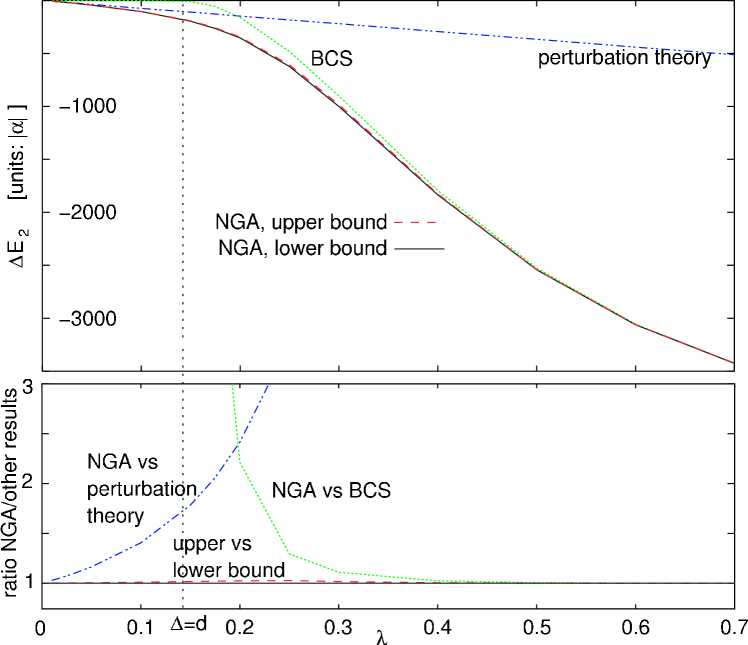
Figure 3: Upper part: The magnetic response $\Delta E_{2}$ from Eq. (7) as function of $\lambda$ for $N=80$ energy levels. The upper and lower bound from the No-Gaudino approximation (solid and dashed line) practically coincide and interpolate between the perturbative and the BCS results (dashed-dotted and dotted line), valid for small and large $\lambda$, respectively.
Lower part: The ratio between the No-Gaudino approximation and the other results. In the regime $\lambda\sim 1/\ln N$, the perturbative and the BCS results underestimate the true result (which must lie between the upper and lower bound) by a factor of more than 2.

As a second example of a quantity that is well captured by the NGA, we calculate the prediction of the pairing Hamiltonian for the magnetic response $\Delta E_{2}$ of small metallic rings footnote (2004), i.e. the derivative of the persistent current with respect to flux at zero flux. For $\lambda\!\ll\!1/\ln N$, $\Delta E_{2}$ was calculated in perturbation theory, for $\lambda\!\gg\!1/\ln N$ the BCS approximation was used Schechter et al. (2002). Here, using the NGA, we calculate $\Delta E_{2}$ for all values of $\lambda>0$, and specifically in the crossover regime between the perturbative and the BCS regimes.

The linear response to the magnetic flux through a ring is given by $\Delta E_{2}=E_{2}^{\mathrm{par}}-E_{2}^{\mathrm{dia}}$, where

$$E_{2}^{\mathrm{par}}\!=\!-2\left(\frac{e}{m_{e}L}\right)^{2}\!\!\!\!\!\sum_{mn,|I\rangle}\!\!\!|P_{mn}|^{2}\frac{|\langle I|c^{\dagger}_{m\uparrow}c^{\phantom{\dagger}}_{n\uparrow}\!\!-\!c^{\dagger}_{n\downarrow}c^{\phantom{\dagger}}_{m\downarrow}|gs\rangle|^{2}}{E_{I}}.$$ (7)

and $E_{2}^{\mathrm{dia}}$ equals the $\lambda=0$ value of $E_{2}^{\mathrm{par}}$ Schechter et al. (2002). Here, $m_{e}$,$e$ are the electron mass and charge, $L$ is the circumference of the ring. $P_{mn}$ is the momentum operator between the disordered 1-particle states, labelled by $m$ and $n$. In the highly diffusive regime ($\omega_{\mathrm{co}}\!<\!1/\tau$, where $\tau$ is the elastic mean free time), which we assume here for simplicity, $|P_{mn}|^{2}\equiv P^{2}$ can be taken to be constant for $m\neq n$, and zero otherwise [Schechter et al., 2003a]. $E_{2}^{\mathrm{par}}$ can then be extracted from the spectral functions for $\hat{O}_{mn\sigma}$ = $c^{\dagger}_{m\sigma}c^{\phantom{\dagger}}_{n\sigma}$.

In the NGA, only the states $|i=m,n;j=n,m\rangle^{0}$ are retained in Eq. (7). Because the contribution of the other states, which are neglected, is always positive, the NGA produces a lower bound for $E_{2}$. An upper bound can be found as well, namely by replacing the energy denominator of Eq. (7) by the energy $E_{mn}^{0}$of the No-Gaudino state, which is known to be smaller than the energy of any other contributing state. Then, the sum over $|I\rangle$ can be eliminated, and the resulting expression for the upper bound is

$$E_{2}^{>}\!=\!\alpha\sum_{m\neq n}\frac{\langle gs|(c^{\dagger}_{n\uparrow}c^{\phantom{\dagger}}_{m\uparrow}\!\!-\!c^{\dagger}_{m\downarrow}c^{\phantom{\dagger}}_{n\downarrow})(c^{\dagger}_{m\uparrow}c^{\phantom{\dagger}}_{n\uparrow}\!\!-\!c^{\dagger}_{n\downarrow}c^{\phantom{\dagger}}_{m\downarrow})|gs\rangle}{E_{mn}^{0}}.$$ (8)

The results of our calculation are presented in Fig. 3, where the upper and lower bound is compared to the perturbative and to the BCS result, given in Schechter et al. (2002). The lower and upper bounds practically coincide (with an error of $<0.5\%$) in the entire parameter regime; this reflects the high accuracy of the NGA. As expected, the perturbative result is reproduced for small $\lambda$ ($\Delta_{\mathrm{BCS}}\ll d$), the BCS result for large $\lambda$ ($\Delta_{\mathrm{BCS}}\gg d$). However, both results underestimate the exact result by a factor of up to $2.5$ in a large intermediate regime (Fig. 3 bottom). Interestingly, we find that the magnetic response is much larger than the BCS value also in a regime in which $\Delta\gg d$, where the BCS approximation is expected to be valid. This is due to a large contribution of the distant levels from $\Delta_{\mathrm{BCS}}$ up to the interaction cutoff, which the BCS approximation neglects. A similarly large contribution from distant levels has previously been found also for the condensation energy Schechter et al. (2001) and single particle properties Schechter et al. (2003b).

We thank V. Ambegaokar, Y. Imry, D. Orgad and A. Schiller for discussions and ackowledge support through ISF grant No. 193/02-1 and “Centers of Excellence”, the DFG program “semiconductors and metal clusters”, and the DIP fund.

References

- (1)
- Cooper et al. (1957) L. Cooper, J. Bardeen, and J. Schrieffer, Phys. Rev. 108 1175 (1957).
- Tinkham (1996) M. Tinkham, Introduction to Superconductivity (McGraw-Hill, New York, 1996).
- von Delft and Ralph (2001) J. von Delft and D. Ralph, Physics Reports 345, 61 (2001).
- Schechter et al. (2001) M. Schechter, Y. Imry, Y. Levinson, and J. von Delft, Phys. Rev. B 63, 214518 (2001).
- Kurland et al. (2000) I. L. Kurland, I. L. Aleiner, and B. L. Altshuler, Phys. Rev. B 62, 14886 (2000).
- Aleiner et al. (2002) I. Aleiner, P. Brouwer, and L. Glazman, Phys. Reports 358, 309 (2002).
- Richardson and Sherman (1964) R. Richardson and N. Sherman, Nucl. Phys. 52, 221 (1964).
- White and Noack (1999) S. White and R. Noack, in Density matrix renormalization: a new numerical method in physics, edited by I. Peschel et al. (Springer, 1999).
- Dukelsky and Sierra (1999) J. Dukelsky and G. Sierra, Phys. Rev. Lett. 83, 172 (1999).
- Sierra and Dukelsky (2000) G. Sierra and J. Dukelsky, Phys. Rev. B 61, 12302 (2000).
- Gobert et al. (2003) D. Gobert, U. Schollwöck, and J. von Delft, cond-mat/0305361, accepted by EPJ B (2004).
- Kühner and White (1999) T.D. Kühner and S. White, Phys. Rev. B 60, 335 (1999).
- Jeckelmann (2002) E. Jeckelmann, Phys. Rev. B 66, 045114 (2002).
- Sierra et al. (2003) J.M. Roman, G. Sierra, and J. Dukelsky, Phys. Rev. B 67, 064510 (2003).
- footnote (2004) For the purposes of the present paper, our calculation of the persistent current using the BCS model should be regarded as a “toy calculation”, whose sole purpose is to illustrate the merits of the NGA within the BCS model. Whether this model can be expected to give a realistic description of real, quasi one-dimensional wires or not (a matter of some controversy Schechter et al. (2003a); Eckern et al. (2004)) is irrelevant for our purposes here.
- Schechter et al. (2003a) M. Schechter, Y. Oreg, Y. Imry, and Y. Levinson, Phys. Rev. Lett. 90, 026805 (2003a).
- Eckern et al. (2004) U. Eckern, P. Schwab, and V. Ambegaokar, cond-mat/0402561 (2004), reply by the authors of Schechter et al. (2003a) is to be published.
- Schechter et al. (2002) M. Schechter, Y. Imry, Y. Levinson, and Y. Oreg, in Towards the Controllable Quantum States, edited by H. Takayanagi et al. (World Scientific, 2003) and cond-mat/0211315.
- Schechter et al. (2003b) M. Schechter, J. von Delft, Y. Imry, and Y. Levinson, Phys. Rev. B 67, 064506 (2003b).