Landau-Zener Tunneling of Bose-Einstein Condensates in an Optical Lattice

Abstract

A theory of the non-symmetric Landau-Zener tunneling of Bose-Einstein condensates in deep optical lattices is presented. It is shown that periodic exchange of matter between the bands is described by a set of linearly coupled nonlinear Schrödinger equations. The key role of the modulational instability in rendering the inter-band transitions irreversible is highlighted.

Introduction.

After the first realization of Bose-Einstein condensation (BEC) in an optical lattice (OL) AK , and subsequent experimental studies of Bloch oscillations and Landau-Zener (LZ) tunneling of matter Morsch1 , numerous theoretical efforts were made to understand and describe these phenomena. In particular, the effect of the nonlinearity on LZ tunneling has been recently studied in Refs. WN ; ZoGa . Those studies, however, are essentially based on the assumption of smallness of the lattice potential in comparison with the recoil energy, which corresponds to a narrow gap in the spectrum of the underlying linear system – i.e., to the case where one can employ a two-mode approximation, where the modes are plane waves. Meanwhile, recent direct experimental observation of the LZ tunneling of a BEC in an OL Morsch2 ; Morsch3 was performed for the range of the potential amplitudes extended till several recoil energies (a deep OL), challenging the existing theory com . In the latter case, the fine structure of Bloch states becomes of crucial importance and leads to a model different from the one proposed in WN ; ZoGa . Although the basic principles of the LZ tunneling are hosted in the linear band structure, the nonlinear interaction makes the phenomenon very different from the one known in solid state physics. Indeed, in the presence of nonlinearity, the Bloch states can become unstable KS and localized states can appear in the gaps between bands (gap-solitons) which can dramatically affect the atomic transfer rate.

The aim of the present paper is to provide a theoretical understanding of the nonlinear interaction and LZ tunneling between the lowest bands of a periodic potential. This is particularly relevant for a deep OL, where the two edges of the lowest forbidden zone have essentially different properties. This approach reveals not only the role of modulational instability (MI) on the atom transfer between zones, but also the effect of (partial) suppression of the MI by the lattice acceleration. Such an understanding is important for appreciating the ramifications of this key linear phenomenon in the presence of nonlinearity and its connection with critical nonlinear instabilities such as the MI. It is also particularly relevant for interpreting recent experiments in this system Morsch2 ; Morsch3 .

Theoretical Approach.

We start with the Gross-Pitaevskii equation for the macroscopic wave function $\psi=\psi({\bf r},t)$:

$$i\hbar\frac{\partial\psi}{\partial t}=-\frac{\hbar^{2}}{2m}\Delta\psi+V_{trap}({\bf r})\psi+V_{latt}({\bf r})\psi+g_{0}|\psi|^{2}\psi\,,$$ (1)

where ${\bf r}=(x,{\bf r}_{\bot})$, $g_{0}=4\pi\hbar^{2}a_{s}/m$, $a_{s}$ is the $s$-wave scattering length, and $m$ is the atomic mass. The trap potentials are given by $V_{trap}({\bf r})=\frac{m}{2}\left(\omega_{x}^{2}x^{2}+\omega_{0}^{2}r_{\bot}^{2}\right)$ and by $V_{latt}({\bf r})=\frac{V_{0}}{2}\cos^{2}\left[\frac{2\pi}{\lambda}\left(x-\frac{a}{2}t^{2}\right)\right]$ where $\omega_{x}$ and $\omega_{0}$ are the harmonic oscillator frequencies, $\lambda$ is the laser wavelength and $a$ is the acceleration of the OL.

In the following we restrict to the weakly nonlinear regime which can be quantified as $\epsilon=(2\sqrt{2}\xi k)^{-1}\ll 1$ where $\xi=(8\pi n|a_{s}|)^{-1/2}$ is the healing length, $k=\frac{2\pi}{\lambda}$, and $n$ is the mean atomic density. To this end, we introduce new variables $X=2k\left(x-\frac{at^{2}}{2}\right)$, ${\bf R}_{\bot}=2k{\bf r}_{\bot}$, and $T=\frac{8E_{R}}{\hbar}t$, where $E_{R}=\frac{\hbar^{2}k^{2}}{2m}$ is the recoil energy, the dimensionless parameters $v=\frac{V_{0}}{16E_{R}}$, $\gamma=\frac{a\hbar^{2}k}{(8E_{R})^{2}}$, and $\nu_{\alpha}=\frac{\hbar\omega_{\alpha}}{4E_{R}}$, $\sigma=$sign$(a_{s})$, and a wave function $\Psi(T,{\bf R})$:

$$\psi(t,{\bf r})=e^{-ivT+i\gamma XT-i\frac{\gamma^{2}}{3}T^{3}+i\frac{\nu_{x}^{2}\gamma^{2}}{40}T^{5}}\sqrt{n}\Psi(T,{\bf R})\,.$$ (2)

Then, Eq. (1) can be rewritten in the form

$$i\partial_{T}\Psi=\frac{1}{2}({\cal L}_{X}+{\cal L}_{\bot})\Psi+\gamma X\left(1+\frac{\nu_{x}^{2}}{2}T^{2}\right)\Psi$$

$$+\frac{\nu_{x}^{2}}{2}X^{2}\Psi+\sigma\epsilon^{2}|\Psi|^{2}\Psi$$ (3)

where ${\cal L}_{X}=-\partial_{X}^{2}+v\cos(X)$ and ${\cal L}_{\bot}=-\Delta_{\bot}^{2}+\nu_{0}^{2}R_{\bot}^{2}.$

For weak nonlinearity the energy of the two-body interaction is much less than the recoil energy and Eq. (Theoretical Approach.) can be reduced to a system of coupled one-dimensional nonlinear Schrödinger equations. To show this we introduce a set of variables $t_{l}=\epsilon^{l}T$, $x_{l}=\epsilon^{l}X$, ($l=0,1,...$) which are considered independent, and look for a solution in the form $\Psi=\psi_{1}+\epsilon\psi_{2}+...$, where $\psi_{j}=\psi_{j}(t_{0},...,x_{0},...,{\bf R}_{\bot})$. After substituting these expansions into (Theoretical Approach.), we single out equations of the same order in $\epsilon$ as: $[i\partial_{t_{0}}-\frac{1}{2}({\cal L}_{x_{0}}+{\cal L}_{\bot})]\psi_{j}=F_{j}$, where $F_{1}=0$, $F_{2}=-i\partial_{t_{1}}\psi_{1},$ etc., and ${\cal L}_{x_{0}}=-\partial_{x_{0}}^{2}+v\cos(x_{0})$. We then consider the eigenvalue problems ${\cal L}_{x_{0}}\varphi_{\alpha q}(x_{0})={\cal E}_{\alpha}(q)\varphi_{\alpha q}(x_{0}),$ and ${\cal L}_{\bot}\zeta_{\mu_{\bot}}=\mu_{\bot}\zeta_{\mu_{\bot}},$ where $\alpha$ characterizes the zone, $q$ is a wave-vector in the first Brillouin zone (BZ), and $\mu_{\bot}$ refers to the transverse quantum numbers.

Focusing on the tunneling (i.e., particle transfer) between the two lowest bands, straightforward algebra shows that if all atoms are initially concentrated in the lowest transverse state, the lattice acceleration does not cause (to leading order) transitions among the transverse levels. This allows us to use $\zeta_{\bot}=(\frac{\nu_{0}}{\pi})^{1/2}\exp(-\frac{\nu_{0}}{2}R_{\bot}^{2})$ and look for the wave function in the form

$$\psi_{1}=e^{-2i\nu_{0}t_{0}}\zeta_{\bot}[A_{1}(x_{1},t_{2})\varphi_{1}+A_{2}(x_{1},t_{2})\varphi_{2}]$$ (4)

where we denoted with $\varphi_{1,2}$ the modes bordering the BZ (i.e. the ones with $q=\pi/2$). Further simplification can be achieved by assuming that the band structure is well pronounced, i.e., that the condensate is wide enough in the $x$-direction, $\hbar\omega_{x}\ll E_{R}$. This is expressed through the rescalings $\nu_{x}=\epsilon^{2}\tilde{\nu}$ and $\gamma=\epsilon^{2}\tilde{\gamma}$ where $\tilde{\nu}\sim\tilde{\gamma}\sim 1$, allowing one to neglect the term proportional to $\gamma\nu_{x}^{2}T^{2}$.

We now use the multiple scale technique (see e.g., KS ) where we take into account the existence of two modes due to tunneling. This leads to the system

$$\begin{array}[]{l}\displaystyle{i\partial_{t_{2}}A_{1}+(2m_{1})^{-1}\partial_{x_{1}}^{2}A_{1}-\beta_{11}A_{1}-\beta_{12}A_{2}}\\ \displaystyle{+(\tilde{\nu}^{2}x_{1}^{2}/2)A_{1}-(\chi_{11}|A_{1}|^{2}+\chi_{12}|A_{2}|^{2})A_{1}=0,}\\ \displaystyle{i\partial_{t_{2}}A_{2}+(2m_{2})^{-1}\partial_{x_{1}}^{2}A_{2}-\beta_{21}A_{1}-\beta_{22}A_{2}}\\ \displaystyle{+(\tilde{\nu}^{2}x_{1}^{2}/2)A_{2}-(\chi_{21}|A_{1}|^{2}+\chi_{22}|A_{2}|^{2})A_{2}=0.}\end{array}$$ (9)

Here $m_{\alpha}^{-1}=\frac{1}{2}\frac{d^{2}{\cal E}_{\alpha}(q)}{dq^{2}}$ are the inverse effective masses,

$$\chi_{ij} = \frac{\sigma\nu_{0}}{4\pi^{2}}\int_{-\pi}^{\pi}|\varphi_{i}(x)|^{2}|\varphi_{j}(x)|^{2}dx$$ (10)

$$\beta_{ij} = \frac{\tilde{\gamma}}{2\pi}\int_{-\pi}^{\pi}x\bar{\varphi}_{i}(x)\varphi_{j}(x)dx.$$ (11)

Recalling that $\varphi_{j}$ border the lowest gap, one concludes that i) $m_{1}<0$ and $m_{2}>0$; ii) $\beta_{11}=\beta_{22}=0$ and $\beta_{12}=\beta_{21}=\beta$, and iii) $\chi_{12}=\chi_{21}=\chi$ (below we use the notation $\chi_{j}=\chi_{jj}$). Then, we end up with the system

$$i\partial_{t_{2}}A_{\alpha}=-(2m_{\alpha})^{-1}\partial_{x_{1}}^{2}A_{\alpha}+\beta A_{3-\alpha}+(\tilde{\nu}^{2}x_{1}^{2}/2)A_{\alpha}$$

$$+(\chi_{\alpha}|A_{\alpha}|^{2}+\chi|A_{3-\alpha}|^{2})A_{\alpha},\quad\alpha=1,2.$$ (12)

Approximating the Bloch functions by $\varphi_{\alpha}(x)=\sqrt{2}\cos(\frac{x+(1-\alpha)\pi}{2})$, we find that $\chi=\frac{\sigma\nu_{0}}{4\pi}$, $\chi_{j}=3\chi$, $\beta=\gamma$.

At this point, it is worth to emphasize the differences between our model and the one used in Refs. WN ; ZoGa . First, in a generic case the nonlinear terms responsible for self-phase and cross-phase modulation appear with different coefficients, respectively $\chi_{1}$ and $\chi$, originating from the different structure of the Bloch functions at two edges of the gap. Unlike the phenomenological model considered in Ref. WN , these terms appear in (Theoretical Approach.) with the same sign. Second, our model includes the group velocity dispersions (i.e. the inverse effective masses) in explicit form, a feature that does not occur in the approximation of a shallow OL. Third, the time does not enter explicitly the equations for the envelopes because it is scaled out by the ansatz (2) using smallness of $\gamma\nu_{x}$, making the resulting system conservative. Finally, our model takes into account the trap potential (an essential ingredient of the experimental setup Morsch2 ; Morsch3 ).

The system (9) leads to a number of conclusions:

(a) In the presence of nonlinearity the LZ tunneling is an asymmetric effect. This stems not only from the fact that the coefficients of the two equations are different i.e., $|m_{1}|^{-1}\neq m_{2}^{-1}$ and $\chi_{1}\neq\chi_{2}$, but also form the fact that the condensate at one gap edge is modulationally stable [edge 2 (1) in the case of a positive (negative) scattering length] and modulationally unstable at the other edge KS .

(b) If, however, one considers the evolution of un-modulated Bloch waves (i.e., the case $\partial_{x_{1}}A_{j}=0$) then the inverse effective masses do not appear in the description of the phenomenon and in a rather common situation when $\chi_{1}\approx\chi_{2}$, the LZ tunneling becomes symmetric. This case can be explicitly treated analytically. The analysis of the resulting equations for the populations of the two bands demonstrates the existence of oscillations of matter between the bands. However, as this case ignores the important feature of MI, we do not discuss it here.

(c) Although Eqs. (9) are coupled for $\gamma=0$, the number of particles ${\cal N}_{j}=\int|A_{j}|^{2}dx_{1}$, is separately preserved (i.e. $d{\cal N}_{j}/dt_{2}=0$ if $\gamma=0$) and LZ tunneling cannot occur in this case. On the contrary, for $\gamma\neq 0$ one has the conservation of the total number of particles ${\cal N}={\cal N}_{1}+{\cal N}_{2}$: $d{\cal N}/dt_{2}=0$ and LZ tunneling can occur.

Numerical Results.

We define the rate characterizing tunneling as $r(t)={\cal N}_{1}/{\cal N}$. In the numerical experiments, we have simulated the 2-state transition model of Eqs. (12) with parameters adapted to the experiments reported in Ref. Morsch2 . In particular, we consider $V_{0}=2.2E_{R}\approx\hbar\times 10^{3}$Hz, corresponding to $v=0.1375$; hence, $m_{1}^{-1}\approx-1.5$ and $m_{2}^{-1}\approx 2.5$ (as obtained from the band structure of the respective potential). A weak magnetic trapping for rubidium atoms has been implemented by choosing $\omega_{x}\approx 2\pi\times 55Hz$ and $\omega_{0}\approx 2\pi\times 200$Hz, which corresponds to $\nu_{x}=0.03$ and $\nu_{0}=0.1$. The nonlinear and linear couplings have been obtained from Eqs. (10)-(11). In particular, $\chi=0.008$ and $\chi_{j}=0.024$, while $\beta$, similarly to the setting of Morsch3 , was varied (typically) in the interval $\beta\in[0.2,1.4]$. Furthermore, the calculations were also performed for solutions of various amplitudes to emulate the variation of the nonlinearity in Morsch3 .

We first examined cases where $A_{1}(x,0)=0$ and the second component is an exact solution of Eq. (12) with $\alpha=2$ and in the absence of linear coupling. Typical results for the transfer rate are shown in Fig. 1.

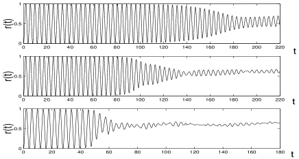
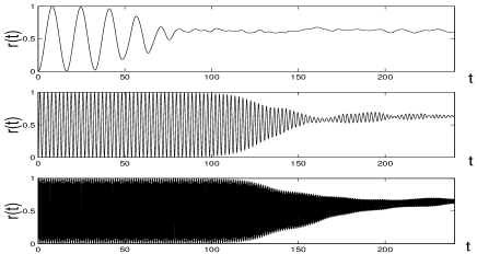
Figure 1: The tunneling ratio $r(t)=N_{1}/N$ is given for three different amplitudes and $\beta=0.8$ on the top three panels: $\max(A_{2}(x,0))=3.22$ (first from the top), $4.83$ (second) and $6.46$ (third). It is also shown for $\max(A_{2}(x,0))=4.83$, for three different couplings $\beta=0.2$ (fourth panel), $1.4$ (fifth) and $10$ (sixth).

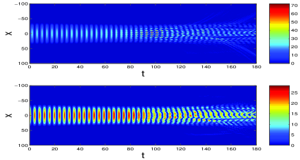
Figure 2: The first two panels from the top show the spatio-temporal contour plots of $|A_{1}(x,t)|^{2}$ (first from the top) and $|A_{2}(x,t)|^{2}$ (second panel). Initially (i.e., at $t=0$) the second component is populated [$\max(A_{2}(x,0))=4.83$], while the first is not. The remaining three panels show three snapshots at different times of the spatial profile of the first (solid line) and of the second (dashed line) component. In the middle and bottom panels the development of the MI is evident.

At the early stages of the dynamical evolution, one observes periodic particle transfer between two bands, reflecting the fact that the probabilities of direct and reciprocal tunneling are the same (an effect not taken into account by the simplified qualitative picture in Morsch3 but also predicted by the model of Ref. ZoGa ). However, after some critical time, $t_{cr}$, the behavior of the system changes drastically: the amplitude of the tunneling rate oscillations decreases substantially, indicating that the system never returns back to the state where all atoms are condensed in only one band. As one can see from the top three panels in Fig. 1, the critical time is smaller for larger initial atomic populations of the second zone i.e., for larger nonlinearity. The remaining panels of Fig. 1 display two other important features: (i) the frequency of oscillations increases with the lattice acceleration and (ii) the critical time also increases with the lattice acceleration. The first of these features seems to be intuitively clear: larger linear force corresponds to larger probability of tunneling and thus to more intensive interchange of atoms between the bands. The second item, as well as the existence of $t_{cr}$ itself, are less evident. In order to appreciate these features, we computed the evolution of the density profiles corresponding to the two bands. Fig. 2 shows the spatio-temporal contour plot (as well as snapshots of time) evolution of the two components for an initial condition with $\max(A_{2}(x,0))=4.83$. Approximately at $t=35$ (for the case $\epsilon^{2}\sim 0.1$, corresponding in physical units to approximately 90 $\mu$s), MI starts to develop in the system and at $t=60$ one can already see a well pronounced periodic structure of the distribution of atoms in the first band, which at $t=90$ develops into a number of solitary pulses, as is typical for MI. The emergence of stable localized states eventually renders the transfer of matter between the two zones irreversible. The time of the development of soliton-like structures coincides with the critical time observed in Fig. 1 (second top panel). This explains the change in the dynamics of the tunneling rate reported above. Namely, the particle exchange between the two bands is suppressed after solitonic (train) structures are developed from the “unstable” band (the lowest band in our case). Notice that the stronger the nonlinearity is, the larger is the region of unstable wavenumbers and equivalently the shorter is the time for the instability development, thus explaining the differences in the tunneling rates shown in Fig. 1. One can also explain the dependence of $r(t)$ on the lattice acceleration (linear force). Indeed, while in the “unstable” band, the nonlinearity tends to fragment the condensate, immediately after transfer to the “stable” band the nonlinearity leads to dispersion of the wave packet. By increasing the linear force ($\beta$) one increases the frequency of oscillations of $r(t)$, i.e., decreases the time atoms spend in the “unstable” band, thus effectively reducing the MI growth rate. This explains the increase of the critical time $t_{cr}$ at which MI develops, observed for increasing $\beta$ in the three bottom panels of Fig. 1; notice from the bottom panel that for very large $\beta$ the effect saturates. In all the cases we observed rather weak dependence of the final upper-to-lower tunneling on the nonlinearity which corroborates the results of Ref. Morsch3 . Our result of the tunneling rate however is larger than the experimentally observed, which, apparently, is an artifact of the two-mode model; the latter does not account for the atoms tunneling to higher bands, thus reducing the effective number of atoms participating in inter-band transfer with respect to the experiment.

The case in which all atoms are initially in the lowest band can be treated similarly. Since, in this case, the homogeneous distributions are unstable, it is natural to start with an initial condition which is a gap soliton resulting from MI and containing the same number of atoms as in the previous case. To understand the phenomenon, we use as initial condition a soliton which is somewhat displaced from the bottom of the potential so that the tunneling matter will be spatially separated from the pulse (due the dynamics in the trap) and therefore easily distinguishable. This setting is illustrated in Fig. 3. As is shown in the snapshot of the bottom right panel of the figure, the wave packets on the left are well separated from the localized pulse. These represent the matter that has tunneled to the second band. Our numerical results indicate that to each burst of matter in the second band, there corresponds one in the first band. Also notice that the burst of matter in the second band (see the top right panel of Fig. 3) is becoming more and more extended as one expects for a Bloch wave of the stable band. The separation of the matter strongly decreases the interaction between the bands (the corresponding wave packets have practically zero overlapping), thus leading to the formation of a plateau in the tunneling rate. The asymptotic tunneling rate achieved in this case may be different from the one obtained in previous case (cf., e.g., Fig. 1); this further supports the existence of an essential asymmetry induced by the nonlinearity in the LZ tunneling .

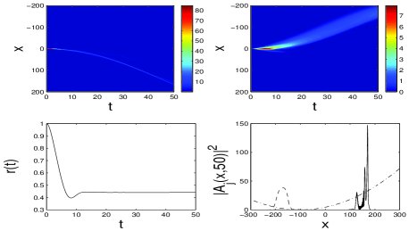
Figure 3: The top left and right panels show space-time contour plots of the 1st and 2nd band wavefunctions respectively. The bottom left shows the temporal evolution of the tunneling ratio $r(t)$, while the bottom right shows a snapshot of the solution at $t=50$. Solid line: $|A_{1}|^{2}$; dashed line: $|A_{2}|^{2}$; dash-dotted: parabolic potential.

Conclusions.

We have provided a systematic derivation of a two-band model reduction relevant to the interaction of the lowest bands of a periodic potential. A theme of particular interest, in this context, is the Landau-Zener tunneling of a BEC between two bands of an optical lattice, a recurring theme of theoretical and experimental importance. While a number of our results, like the sensitivity of the effect with respect to initial distributions, the oscillatory behavior of tunneling rate, and the qualitative symmetry with respect to exchange of bands $1\leftrightarrow 2$ with simultaneous change of the sign of the scattering length corroborate the predictions of ZoGa , we have illustrated important differences from previously explored models and have highlighted the asymmetric nature of the tunneling and the important role of the nonlinearity through the modulational instability in the process. These results illustrate the importance of (experimentally) studying this system for longer times substantially larger than the critical time (and/or stronger nonlinearities) to appreciate the role of the nonlinearity in modifying the classical picture of the Landau-Zener tunneling.

VVK is grateful to O. Morsch for stimulating discussions. PGK acknowledges support from NSF-DMS-0204585, NSF-CAREER and the Eppley Foundation for Research. MS acknowledges financial support from a MURST-PRIN-2003 Initiative.

References

- (1) B. P. Anderson and M. A. Kasevich, Science 282, 1686 (1998)
- (2) O. Morsch, et al. Phys. Rev. Lett. 87, 140402 (2001).
- (3) B. Wu and Q. Niu, Phys. Rev. A 61, 023402 (2000); J. Liu et al. Phys. Rev. A 66, 023404 (2002).
- (4) O. Zobay and B. M. Garraway, Phys. Rev. A 61, 033603 (2000).
- (5) M. Jona-Lasinio, et al. Phys. Rev. A 65, 063612 (2002).
- (6) M. Jona-Lasinio et al. Phys. Rev. Lett. 23, 230406 (2003).
- (7) Experimental upper-to-lower band tunneling rates are lower than the ones for the reciprocal tunneling (see, Figs. 2b and 3 of Morsch3 ). This does not agree with the theoretical predictions, stating the opposite (see Fig. 2a of Morsch3 ).
- (8) V. V. Konotop and M. Salerno, Phys. Rev. A 65 021602 (2002).