Orthogonality Catastrophe in Bose-Einstein Condensates

Abstract

Orthogonality catastrophe in fermionic systems is well known: in the thermodynamic limit, the overlap between the ground state wavefunctions with and without a single local scattering potential approaches zero algebraically as a function of the particle number $N$. Here we examine the analogous problem for bosonic systems. In the homogeneous case, we find that ideal bosons display an orthogonality stronger than algebraic: the wavefunction overlap behaves as ${\rm exp}[-\lambda N^{1/3}]$ in three dimensions and as ${\rm exp}[-\lambda N/\ln^{2}N]$ in two dimensions. With interactions, the overlap becomes finite but is still (stretched-)exponentially small for weak interactions. We also consider the cases with a harmonic trap, reaching similar (though not identical) conclusions. Finally, we comment on the implications of our results for spectroscopic experiments and for (de)coherence phenomena.

In the area of correlated electrons, there is a long history of studying quantum impurity problems such as the Kondo effect Hewson . A broad range of phenomena arise depending on the type of impurity, the nature of the bulk electron system, and the way they are coupled. The conceptual basis for this richness is provided by the orthogonality catastrophe Anderson . It deals with the effect of a single scattering potential on the many-body states of an ideal $N$-fermion system. The many-body ground state wavefunction is a Slater determinant of the $N$ lowest single particle wavefunctions. Since the impurity potential affects each and every one of the single-particle states, its effect on the many-body state is significantly amplified: in the thermodynamic limit the ground state wavefunction in the presence of the impurity potential ($|{\rm gs}^{\prime}>$) is orthogonal to its counterpart in the absence of the impurity potential ($|{\rm gs}>$). For large but finite $N$, the wavefunction overlap, $S\equiv|<{\rm gs}|{\rm gs}^{\prime}>|$, depends on $N$ in an algebraic form:

$$S_{\rm fermion}\sim N^{-\alpha}.$$ (1)

The exponent $\alpha=\delta^{2}/d\pi^{2}$ when the scattering contains only an s-wave component; here, $\delta$ is the $s-$wave scattering phase shift of the single-particle state at the Fermi energy, and $d$ the dimensionality. The initial work of Anderson provided an upper bound. An exact solution was later achieved in the work of Nozières and collaborators Nozieres . For an illuminating discussion, including the connection with the Friedel sum rule, see Ref.  Hopfield .

Cold atoms provide a setting to engineer many-boson systems with a variety of quantum phases Greiner . It is natural to ask what happens when local defects are introduced into these systems. Here we consider the orthogonality effect in a Bose-Einstein condensate (BEC). For ideal homogeneous bosons, the problem will be solved exactly in a very simple way. For the cases with interactions and/or confining background potentials, we will carry out analyses perturbatively in the impurity potential.

Ideal bosons in a uniform background:   In this case, the effect of an impurity can be determined exactly. The ground state condensate wavefunction is

$$|{\rm gs}>=\varphi_{0}({\bf x}_{1})\varphi_{0}({\bf x}_{2})...\varphi_{0}({\bf x}_{N}),$$ (2)

where $\varphi_{0}$ is the single-particle ground state wavefunction. $|{\rm gs}^{\prime}>$ has the same form, with $\varphi_{0}$ being replaced by $\varphi_{0}^{\prime}$, the single-particle ground state wavefunction in the presence of the impurity. The overlap, $S$, is then simply

$$S = s^{N}$$ (3)

$$s \equiv <\varphi_{0}|\varphi_{0}^{\prime}>$$ (4)

Consider first the case of three dimensions. We choose a spherical box of radius $R$, and a fixed boundary condition $\varphi(r=R)=0$. The impurity is placed at the center:

$$\Delta H=V\Theta(a-r)$$ (5)

where $a$ is its size. Without a loss of generality, the potential will be taken as repulsive. we define $\psi$ as the radial part of the single-particle wavefunction multiplied by $r$. In the region $0<r<a$, ${\psi_{I}}=A\sin({k_{I}}r)$, with ${k_{I}}^{2}=\frac{2m}{{\hbar}^{2}}(\epsilon-V)$. In the region $a<r<R$, ${\psi_{II}}=B\sin({k_{II}}r+\delta)$, with ${k_{II}}^{2}=\frac{2m}{{\hbar}^{2}}\epsilon$, where $\delta$ is the phase shift. The fixed boundary condition at $r=R$ yields $k_{II}=\frac{\pi-\delta}{R}$. The continuity of $\psi$ and its derivative at $r=a$ gives rise to

$$\frac{\tan({k_{I}}a)}{k_{I}}=\frac{\tan({k_{II}}a+\delta)}{k_{II}}$$ (6)

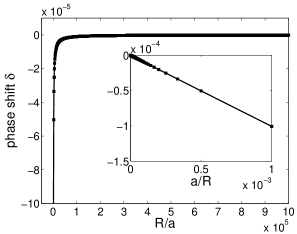
Figure 1: Phase shift as a function of the system size in three dimensions, with $\bar{V}=0.1$. Inset: the phase shift vs. $a/R$

The phase shift for the single-particle ground state in the thermodynamic limit ($R/a\rightarrow\infty$) is found to be

$$\delta_{3d}=-\frac{a}{R}f(V)$$ (7)

where $f(V)=\pi(1-\frac{\tanh(\bar{V})}{\bar{V}})$, with ${\bar{V}}\equiv(\frac{2mVa^{2}}{{\hbar}^{2}})^{1/2}$. The $a/R$ dependence reflects the fact that the single particle state sits at the edge of the band, where the density of states is proportional to $\sqrt{\epsilon}\propto a/R$. The numerical result [Fig. 1] shows the validity of this form already for $R/a$ of the order $10^{3}$.

From the forms of the wavefunctions in the presence and in the absence of the impurity, we determine the overlap of the single-particle wavefunctions

$$s=1-{1\over 6}(1+{3\over{4\pi^{2}}})\delta_{3d}^{2},$$ (8)

where we have used the fact that $\delta_{3d}$ is always small in the thermodynamic limit. Combining Eqs. (3,8,7), we find a stretched-exponential form for the overlap of the many-body ground states:

$$S_{\rm 3d}={\rm exp}[-\lambda(V)N^{1/3}]$$ (9)

where $\lambda(V)=\frac{1}{6}(1+\frac{3}{4\pi^{2}})a^{2}f^{2}(V)\left(\frac{4\pi n_{0}}{3}\right)^{\frac{2}{3}}$, with $n_{0}$ being the particle density.

Consider next the case of two dimensions – a disk of radius $R$. The ground state wavefunction $\psi$ is now a linear combination of the zeroth order Bessel and Neumann functions: $\psi_{I}=AJ_{0}(k_{I}r)$ and $\psi_{II}=B[J_{0}(k_{II}r)+\tan(\delta)N_{0}(k_{II}r)]$. The fixed boundary condition at $r=R$ now gives $k_{II}=\frac{\frac{3\pi}{4}+\delta}{R}$. The continuity at $r=a$ of $\psi$ and its derivative leads to

$$\frac{k_{I}J_{1}(k_{I}a)}{J_{0}(k_{I}a)}=\frac{k_{II}[J_{1}(k_{II}a)+\tan(\delta)N_{1}(k_{II}a)]}{J_{0}(k_{II}a)+\tan(\delta)N_{0}(k_{II}a)}$$ (10)

Using the limiting forms of the Bessel and Neumann functions appropriate for $a/R\rightarrow 0$, we find the following phase shift of the single-particle ground state

$$\delta_{\rm 2d}=\frac{\pi}{2}\frac{1}{\ln(R/a)}.$$ (11)

Note that it is independent of the potential strength. The finite value of the density of states at the band edge would have implied a phase shift that is independent of $R/a$. The exact result, on the other hand, contains a logarithmic correction factor. In Fig. 2, we plot the numerical solution which confirms the logarithmic factor.

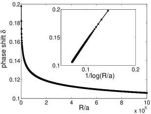
Figure 2: The analogous plot for two dimensions, with $\bar{V}=1$. Inset: phase shift vs. $1/\ln(R/a)$.

Taking these results together we find the overlap of the many-body ground states in two dimensions:

$$S_{\rm 2d}={\rm exp}[-\alpha N/\ln^{2}N],$$ (12)

where $\alpha=\frac{\pi^{2}}{2}\left[\frac{\int B^{2}(x)}{\int J_{0}^{2}(\frac{3\pi}{4}x)}-5\left(\frac{\int J_{0}(\frac{3\pi}{4}x)B(x)}{\int{J_{0}}^{2}(\frac{3\pi}{4}x)}\right)^{2}\right]$, with $B(x)=N_{0}(\frac{3\pi}{4}x)-J_{1}(\frac{3\pi}{4}x)x$ and $\int f(x)\equiv\int_{0}^{1}f(x)xdx$.

So far, the results are exact. In order to generalize to situations in which exact solutions are not readily available (see below), we now turn to a perturbative treatment of the impurity potential. To the second order in a linked cluster expansion, the overlap between the many-body ground state wavefunctions is Mahan :

$$S = {\rm exp}[-C]$$

$$C = \frac{1}{2}\sum_{n\neq{\rm gs}}{{|<n|\Delta H|{\rm gs}>|^{2}}\over{(E_{n}-E_{\rm gs})^{2}}}.$$ (13)

The impurity scattering can be rewritten as $\Delta H=Va^{\dagger}({\bf x}={\bf 0})a({\bf x}={\bf 0})$, where $a^{\dagger}({\bf x})$ and $a({\bf x})$ are the boson field operators. The off-diagonal long-range order of a BEC implies that we can set $a_{0}$ and $a_{0}^{\dagger}$ to be $\sqrt{N}$. The impurity Hamiltonian becomes $\Delta H=\Delta H_{1}+V/L^{d}(N+\sum_{{\bf p}\neq{\bf 0}\neq{\bf p^{\prime}}}a_{\bf p}^{\dagger}a_{\bf p^{\prime}})$, where the part of concern to us is

$$\Delta H_{1}=V{\sqrt{N}\over L^{d}}\sum_{{\bf p}\neq{\bf 0}}(a_{\bf p}^{\dagger}+a_{\bf p})$$ (14)

Here, $L$ is the linear dimension of the system. Combining Eqs. (13,14), and using the dispersion relation $\epsilon({\bf p})=p^{2}/2m$, we have

$$C=\frac{V^{2}}{2}{N\over L^{d}}\frac{(2m)^{2}}{(2\pi\hbar)^{d}}\int_{\hbar\pi/L}^{\infty}d^{d}{\bf p}~{}p^{-4}.$$ (15)

In three dimensions, $C$ has a divergence of the form $L\propto N^{1/3}$, which is the same as the exact result [Eq. (9)]. (For the spherical box geometry considered earlier, the perturbative result is found to fully agree with what comes out of Eq. (9) when $\lambda(V)$ is expanded to order $V^{2}$.) In two dimensions, the divergence becomes $L^{2}\propto N$. Compared with the exact result [Eq. 12], the perturbative result recovers the $N$ factor in the exponential but misses the multiplicative logarithmic correction.

The perturbative treatment also provides the physical picture for our results. To see this, we rewrite the expression for $C$ in terms of the dissipation spectral function, $Im\chi_{0}^{-1}(\omega)$, as follows,

$$C = \frac{1}{2}\int_{(E_{1}-E_{\rm gs})}^{\infty}d\omega{{{\rm Im}\chi_{0}^{-1}(\omega)}\over\omega^{2}}$$ (16)

$${\rm Im}{\chi_{0}^{-1}(\omega)} = \sum_{n\neq{\rm gs}}|<n|\Delta H|{\rm gs}>|^{2}\times$$ (17)

$$\times\delta(\omega-E_{n}+E_{\rm gs})$$

where $E_{1}$ is the energy of the first excited state with a non-zero $<n|\Delta H|{\rm gs}>$. The form of the impurity potential, Eq. (14) implies that the dissipation spectral function is simply proportional to the single-particle density of states:

$${\rm Im}\chi_{0}^{-1}(\omega>0)\propto\omega^{{d\over 2}-1}.$$ (18)

The exponent $({d\over 2}-1)$ reflects the quadratic nature of the dispersion of the low-lying excitations. It is less than $1$ for both three and two dimensions; in the terminology adopted in the dissipated two-level system literature Leggett , both are sub-ohmic Kirchner . This abundance of low-lying excitations is responsible for the strong orthogonality in a BEC.

Weakly interacting bosons in a uniform background:   Unlike for fermions, even weak interaction is a relevant perturbation for bosons. We use the standard Bogoliubov transformation Bogoliubov ; Lifshitz ,

$$a_{\bf p}={1\over\sqrt{1-L_{\bf p}^{2}}}[b_{\bf p}+L_{\bf p}b_{-{\bf p}}^{\dagger}].$$ (19)

Under this transformation, the quadratic part of the Hamiltonian becomes

$$H_{0}=\sum_{{\bf p}\neq{\bf 0}}\xi({\bf p})b_{\bf p}^{\dagger}b_{\bf p}.$$ (20)

For $p\gg 2mu$ (where $u=\sqrt{Un_{0}/m}$ is the sound velocity, with $U$ being the effective contact interaction amplitude), $L_{\bf p}$ nearly vanishes and we recover the non-interacting limit, including Eq. (14) and $\xi({\bf p})\approx\epsilon({\bf p})$. For $p\ll 2mu$, on the other hand, $L_{\bf p}\approx-1+p/mu$, and it follows that

$$\xi({\bf p}) = up$$

$$\Delta H_{1} = V{\sqrt{N}\over L^{d}}\sum_{{\bf p}\neq{\bf 0}}{}^{\prime}\sqrt{{p}\over{2mu}}(b_{\bf p}^{\dagger}+b_{\bf p}),$$ (21)

where the prime denotes that the summation is up to about $2mu$. Eq. (15) is then replaced by

$$C \approx{V^{2}\over{2}}{N\over L^{d}}{1\over(2\pi\hbar)^{d}}(2m)^{2}\times$$ (22)

$$\times\left[\frac{1}{(2mu)^{3}}\int_{\hbar\pi/L}^{2mu}d^{d}{\bf p}~{}p^{-1}+\int_{2mu}^{\infty}d^{d}{\bf p}~{}p^{-4}\right].$$

It is convergent in both three and two dimensions, implying a finite wavefunction overlap. The resulting overlap in the thermodynamic limit depends on the interaction $U$ in the following (stretched-)exponential forms:

$$S_{\rm U,3d}={\rm exp}[-\lambda^{\prime}/\sqrt{U}]$$

$$S_{\rm U,2d}={\rm exp}[-\alpha^{\prime}/U]$$ (23)

where $\lambda^{\prime}\approx\frac{V^{2}\sqrt{n_{0}}m^{3/2}}{4\pi^{2}\hbar^{3}}$ and $\alpha^{\prime}\approx\frac{3V^{2}m}{8\pi\hbar^{2}}$.

This conclusion can also be seen through the form of the dissipative-bath spectral function, which, at low-energies, now takes the form [cf. Eqs. (17,21)]

$${\rm Im}\chi_{0}^{-1}(\omega>0)\propto\omega^{d}.$$ (24)

Its super-ohmic nature in two and three dimensions implies that $C$ [cf. Eq. (16)] is infrared convergent Leggett .

Ideal bosons in a harmonic confining potential:   Consider an isotropic harmonic trap with frequency $\Omega_{0}$. The thermodynamic limit is defined by keeping

$$N\Omega_{0}^{d}={\rm const.}$$ (25)

as both $N$ and $1/\Omega_{0}$ go to infinity Dalfovo . (For instance, it ensures a finite energy per particle for ideal fermions.)

We consider an impurity located at the center of the trap: $\Delta H=Va^{\dagger}({\bf x=0})a({\bf x=0})$. Using $a({\bf x})=\sum_{\bf n}\varphi_{\bf n}({\bf x})a_{\bf n}$, where ${\bf n}\equiv(n_{1},\cdot\cdot\cdot,n_{d})$, and the single-particle eigenfunctions

$$\varphi_{\bf n}({\bf x}) = \left({{m\Omega_{0}}\over{2\hbar}}\right)^{d/4}\Pi_{i=1}^{d}(n_{i}!)^{-{1\over 2}}\left({{m\Omega_{0}}\over{2\hbar}}\right)^{{n_{i}\over 2}}\times$$ (26)

$$\times\left(x_{i}-{\hbar\over{m\Omega_{0}}}{d\over{dx_{i}}}\right)^{n_{i}}{\rm e}^{-m\Omega_{0}r^{2}/2\hbar},$$

we write the linear part of the impurity Hamiltonian as

$$\Delta H_{1} = V\sqrt{{N}{\Omega_{0}}^{d}}\sum_{{\bf n}\neq{\bf 0}}A_{2{\bf n}}(a_{2{\bf n}}^{\dagger}+a_{2{\bf n}}).$$ (27)

Here, we have defined

$$A_{2{\bf n}}\equiv\frac{\varphi_{2{\bf n}}^{*}(0)\varphi_{\bf 0}(0)}{\Omega_{0}^{d/2}}=\frac{(-1)^{\sum_{i=1}^{d}n_{i}}}{(\pi\hbar/m)^{d/2}}\prod_{i=1}^{d}\left[{{(2n_{i}-1)!!}\over{(2n_{i})!!}}\right]^{{1}\over{2}}.$$ (28)

From Eq. (13), we have

$$C=\frac{V^{2}}{2}(N\Omega_{0}^{d}){1\over(\hbar\Omega_{0})^{2}}\sum_{{\bf n}\neq{\bf 0}}{A_{2{\bf n}}^{2}\over(2n)^{2}},$$ (29)

where $n=\sum_{i=1}^{d}n_{i}$. At large $n$, we find that $\sum_{n_{1},\cdot\cdot\cdot,n_{d}}\delta(n-\sum_{i=1}^{d}n_{i})A_{2{\bf n}}^{2}$ is proportional to $\sqrt{n}$ in three dimensions and approaches a constant in two dimensions sterling , so the summation over $n$ in Eq. (29) is convergent at ultraviolet. $C$ is then proportional to $\Omega_{0}^{-2}$, which, using the thermodynamic limit, is equivalent to $N^{2/d}$. The overlap between the ground state wavefunctions is then

$$S_{\rm ho,3d} \propto {\rm exp}[-\lambda_{ho}N^{2/3}]$$

$$S_{\rm ho,2d} \propto {\rm exp}[-\alpha_{ho}N]$$ (30)

where $\lambda_{ho}=\frac{V^{2}}{4\sqrt{\pi}}\zeta(\frac{3}{2})(m/\pi\hbar^{2})^{3}(N\hbar^{3}\Omega_{0})^{\frac{1}{3}}$ and $\alpha_{ho}=V^{2}(m/\hbar^{2})^{2}/48$.

Weakly-interacting bosons in a harmonic confining potential:   To understand the effect of interactions, we first note on one important consequence of the thermodynamic limit, Eq. (25). In the non-interacting case, it is seen, from the ground state wavefunction $\varphi_{\bf 0}({\bf x})=\left({{m\Omega_{0}}/{\pi\hbar}}\right)^{d/4}{\rm e}^{-m\Omega_{0}r^{2}/2\hbar}$, that the central density of the condensate, $n({\bf x}={\bf 0})\equiv N|\varphi_{0}({\bf x}={\bf 0})|^{2}$, is of the order of $\sqrt{N}$ in the thermodynamic limit.

In the interacting case, on the other hand, $n({\bf x}={\bf 0})$ is well-known to be of order unity in the thermodynamic limit Dalfovo . In this limit, the interaction term dominates over the kinetic term Baym . It follows from the Gross-Pitaevskii equation that $n({\bf x}={\bf 0})=\mu/U$ where the chemical potential $\mu$ is finite in the thermodynamic limit. This implies that $\varphi_{0}({\bf x}={\bf 0})$ in the interacting case is a factor of $N^{-1/4}$ smaller than its counterpart in the non-interacting case. The wavefunctions of the low-lying excited states should contain a similar reduction factor. On the other hand, the energies of the collective modes remain linear in $\Omega_{0}$. It follows [cf. Eqs. (13,27,28)] that interactions weaken the orthogonality effect, as in the uniform case. The precise form of the overlap depends on the details of the excited-state wavefunctions, which can be determined from the Bogoliubov-de Gennes equations in a harmonic potential; this will be discussed elsewhere.

Experimental implications:   In addition to the theoretical significance, the orthogonality effect may also be directly probed in experiments. One way is to perform the analog of the x-ray edge measurement in metals Hopfield ; Mahan . Consider a condensate co-existing with a separate species of atoms that are considerably more dilute and are localized (by a deep optical potential well that only these atoms see). The photo-absorption or luminescence corresponding to a transition between two levels of this second species of atoms would ordinarily be a sharp delta function. (In practice, the spectral width of a hyperfine transition for atoms in a BEC can be as narrow as $\sim$100 Hz or even $\sim$10 Hz Hulet .) However, the two atomic levels will provide different scattering potentials for the atoms of the condensate. The weight of the delta function – which is precisely the overlap of the condensate wavefunctions corresponding to these two different potentials – would then have to vanish in the thermodynamic limit due to the orthogonality catastrophe. A finite spectral weight can arise only when the condensate atoms go to the excited states under the new potential, where the excitation energy serves as a cutoff for the infrared divergence. This results in a one-sided spectrum Hopfield , which can be divergent or vanishing at the edge depending on the degree of orthogonality for the low-lying excited states.

The orthogonality may also be manifested in the time evolution of a condensate after a sudden introduction of a local potential. The orthogonality makes it rather hard for the system to evolve into the new ground state. In other words, the density distribution will tend to keep its initial profile; the impurity is “hardly visible” to the condensate.

Yet another implication is on the coherence and decoherence phenomena. Consider, for instance, localized atoms in a BEC. An effective Kondo problem arises when both the localized atoms as well as the itinerant atoms of the condensate contain real or pseudo- spin degrees of freedom Zwerger ; Cirac . Strong orthogonality makes the spin flip process entirely incoherent.

To summarize, we have studied the orthogonality effect in Bose-Einstein condensates. For ideal bosons, the overlap of the ground state wavefunctions when a single local scattering potential changes from one value to another vanishes in a stretched-exponential form in the thermodynamic limit. With interactions, the overlap becomes finite but is small for weak interactions; its dependence on the interaction strength is typically stretched-exponential as well. These effects can be probed using spectroscopic experiments in cold atoms, which can be tuned from being essentially ideal to strongly interacting. The effects also have significant implications for the coherence and decoherence phenomena in bosonic systems.

We would like to thank E. Abrahams, P. W. Anderson, K. Damle, R. Hulet, H. Pu and, in particular, C. M. Varma for useful discussions. The work has been supported by NSF Grant No. DMR-0090071 and the Robert A. Welch Foundation.

References

- (1) A. C. Hewson, The Kondo Problem to Heavy Fermions (Cambridge Univ. Press, Cambridge, 1993).
- (2) P. W. Anderson, Phys. Rev. Lett. 18, 1049 (1967).
- (3) P. Nozières and C. T. De Dominicis, Phys. Rev. 178, 1097 (1969). See also B. Roulet, J. Gavoret, and P. Nozières, ibid., 1072 (1969); P. Nozières, J. Gavoret, and B. Roulet, ibid., 1084 (1969).
- (4) J. J. Hopfield, Comm. Solid State Phys. 2, 40 (1969).
- (5) M. Greiner et al., Nature (London) 415, 39 (2002).
- (6) G. D. Mahan, Many-Particle Physics, 2nd ed. (Plenum Press, New York, 1990).
- (7) A. J. Leggett et al., Rev. Mod. Phys. 59, 1 (1987).
- (8) The sub-ohmic form also arises from spin waves of a ferromagnet, which come into play in a different context (S. Kirchner, L. Zhu, Q. Si, and D. Natelson, in preparation).
- (9) N. Bogoliubov, J. Phys. USSR 11, 23-32 (1947).
- (10) E. M. Lifshitz and L. P. Pitaevskii, Statistical Physics part 2 (Butterworth-Heinenann, Oxford, 1995), Sec. 25.
- (11) F. Dalfovo et al., Rev. Mod. Phys. 71, 463 (1999).
- (12) It is important to use the strong form of Sterling’s formula, , which implies .
- (13) G. Baym and C. Pethick, Phys. Rev. Lett. 76, 6 (1996).
- (14) S. Stringari, Phys. Rev. Lett. 77, 2360 (1996).
- (15) R. Hulet, private communications.
- (16) A. Recati, P. O. Fedichev, W. Zwerger, J. von Delft and P. Zoller, cond-mat/0212413.
- (17) B. Paredes, C. Tejedor, and J. I. Cirac, cond-mat/0306497.