Perturbative corrections to the Gutzwiller mean-field solution of the Mott-Hubbard model

Abstract

We study the Mott-insulator transition of bosonic atoms in optical lattices. Using perturbation theory, we analyze the deviations from the mean-field Gutzwiller ansatz, which become appreciable for intermediate values of the ratio between hopping amplitude and interaction energy. We discuss corrections to number fluctuations, order parameter, and compressibility. In particular, we improve the description of the short-range correlations in the one-particle density matrix. These corrections are important for experimentally observed expansion patterns, both for bulk lattices and in a confining trap potential.

I Introduction

The Mott-Hubbard model of interacting bosons on a lattice has been used to describe superfluid Mott-insulator transitions in a variety of systems, e.g., Josephson arrays and granular superconductors Fisher01 . The recent suggestion Jaksch01 to experimentally observe this transition in a system of cold bosonic atoms in an optical lattice and its successful experimental demonstration Greiner01 has rekindled the interest in the Mott-insulator transition and triggered a great deal of theoretical Jaksch02 ; Jaksch03 ; Hofstetter ; Altman ; Zwerger01 ; Buechler01 ; Damski ; Kleinert01 ; Burnett ; Jaksch04 ; Buechler02 ; Lewenstein and experimental Greiner02 ; Mandel01 ; Esslinger activity. The possibility to directly manipulate and test the many-body behavior of a system of trapped bosonic atoms in an optical lattice Greiner02 ; Mandel01 is very attractive. Possible applications include the use of a Mott state of bosonic atoms in an optical lattice as a starting point to create controlled multiparticle entanglement as an essential ingredient for quantum computation Jaksch02 ; Mandel01 ; Briegel01

The Mott-insulator quantum phase transition is driven by the interplay of the repulsive interaction of bosons on the same lattice site and the kinetic energy. Hence the ratio of the onsite energy and the bandwidth forms the key parameter in the system. In optical lattices, this parameter can be easily controlled and varied by several orders of magnitude, enabling detailed studies of the quantum phase transition. Probing the system by taking absorption pictures to image the expansion patterns after a reasonable expansion time yields information about the momentum distribution of the state. This procedure was used to experimentally confirm the Mott transition in an optical lattice Greiner01 .

The essential physics of cold bosonic atoms in an optical lattice is captured by a bosonic Mott-Hubbard model describing the competition between hopping and on-site interaction. A number of approximation schemes have been used to study this model analytically Fisher01 ; Freericks01 ; Oosten01 ; Rey01 as well as numerically, using approaches like the Gutzwiller mean-field ansatz Rokhsar01 ; Jaksch01 , density-matrix renormalization group (DMRG) Kuehner01 ; Rapsch01 ; Kollath01 , exact diagonalization (ED)Roth01 ; Roth02 and Quantum Monte Carlo (QMC) Scalettar01 ; Batrouni01 ; Krauth ; Kisker01 ; Kashurnikov01 .

In this article, we study the short-range correlations, not included by the Gutzwiller ansatz, by using perturbation theory. The main purpose is to find corrections to the short-range behavior of the one-particle density matrix, which is directly relevant to experimentally observed expansion patterns. These patterns are important for determining the location of the insulator-superfluid transition. We note that in the insulating state our perturbative approach is identical to the one used in Freericks01 (see also Elstner ), although there the goal was different, viz., studying corrections to the phase diagram.

The remainder of the article is organized as follows: In Section II, we will introduce the model and its mean-field solution. The general perturbative approach is briefly outlined in Section III, while details may be found in the Appendix. Numerical results are presented and discussed in Section IV, first for local observables (IV.1) and then for the density matrix (IV.2). Implications for expansion patterns both for bulk systems and a harmonic confining potential are discussed in Section IV.3.

II The model

The cold bosonic gas in the optical lattice can be described by a Mott-Hubbard model Jaksch01

$$H=\sum_{i=1}^{M}\frac{U}{2}n_{i}(n_{i}-1)+\sum_{i=1}^{M}\left(\epsilon_{i}-\mu\right)n_{i}-J\sum_{\langle i,j\rangle}a_{i}^{\dagger}a_{j}\,.$$ (1)

Here, $M$ is the total number of lattice sites, $a_{i}^{\dagger}$ ($a_{i}$) creates (annihilates) a boson on site $i$, $n_{i}=a_{i}^{\dagger}a_{i}$, $U$ is the on-site repulsion describing the interaction between bosons on the same lattice site, and $\mu$ denotes the chemical potential. The kinetic term includes only hopping between nearest-neighbor sites, this is denoted by the summation index $\langle i,j\rangle$; $J$ is the hopping matrix element that we will assume to be lattice-site independent. Finally, $\epsilon_{i}$ describes an external on-site potential that is commonly present in experiments.

The Gutzwiller (GW) approach is based on an ansatz for the many-body ground state that factorizes into single lattice-site wavefunctions

$$|G_{0}\rangle=\prod_{i=1}^{M}\left(\sum_{n=0}^{\infty}f_{n}^{(i)}|n_{i}\rangle\right)\,.$$ (2)

The Gutzwiller wavefunction represents the ground state of the following mean-field version of the Mott-Hubbard Hamiltonian, Eq. (1):

$$\begin{split}H_{\mathrm{MF}}&=\sum_{i=1}^{M}\frac{U}{2}n_{i}(n_{i}-1)+\sum_{i=1}^{M}\left(\epsilon_{i}-\mu\right)n_{i}\\ &-J\sum_{\langle i,j\rangle}\left(a_{i}^{\dagger}\Psi_{j}+\Psi_{i}^{*}a_{j}-\Psi_{i}^{*}\Psi_{j}\right)\,.\end{split}$$ (3)

Here $\Psi_{i}$ is the mean-field potential on the $i$-th lattice site, which is self-consistently defined as the expectation value of $a_{i}$ in terms of the Gutzwiller wavefunction, $\Psi_{i}=\langle G_{0}|a_{i}|G_{0}\rangle$ Sheshadri01 .

Using the Gutzwiller ansatz to obtain an approximate variational solution for the Mott-Hubbard Hamiltonian (1) corresponds, however, to restricting the Hilbert space to the subset of product states. Consequently, even in higher dimensions, this ansatz fails to describe the correct behavior of short-range correlations between different lattice sites, which are important for experimentally measurable observables, such as expansion patterns (momentum distributions). Nevertheless, in the thermodynamic limit and higher dimensions, the Gutzwiller wavefunction provides a good approximation in the limits of $J\rightarrow 0$ and $U\rightarrow 0$ (i.e., deep in the Mott insulator (MI) and superfluid (SF) phases). To get a satisfactory description of the short-range correlations we will now derive perturbative corrections to the Gutzwiller mean-field result.

III Perturbative Approach

Our aim is to start from the Gutzwiller approximation and improve it by perturbatively including the short-range correlations between lattice sites. We re-express the Mott-Hubbard Hamiltonian (1) by adding the appropriate perturbation to the mean-field Hamiltonian, Eq. (3):

$$H=H_{\mathrm{MF}}+V\,,$$ (4)

with

$$V=-J\sum_{\langle i,j\rangle}(a_{i}^{\dagger}-\Psi_{i}^{*})(a_{j}-\Psi_{j})\,.$$ (5)

As the mean-field Hamiltonian represents a sum of single lattice-site Hamiltonians, the excited states $|i_{\alpha}\rangle$ and the excitation spectrum $\epsilon^{(i,\alpha)}$ can be obtained numerically for each lattice site $i$ separately. Hence we can write the excitations of $H_{\mathrm{MF}}$ as product states of single lattice-site excitations,

$$|G^{\alpha}\rangle=\prod_{i=1}^{M}|i_{\alpha_{i}}\rangle\,,$$ (6)

and the excitation spectrum as a sum over the single lattice-site excitation energies,

$$\epsilon^{\alpha}=\sum_{i=1}^{M}\epsilon^{(i,\alpha_{i})}\,,$$ (7)

where $\alpha=(\alpha_{1},\alpha_{2},\ldots)$ describes the set of quantum numbers characterizing the given many-body energy eigenstate.

Having obtained the mean-field solution from the Gutzwiller ansatz, we can now proceed to improve our wavefunction performing Rayleigh-Schrödinger perturbation theory tannoudji01 in $V$:

$$\begin{split}&\langle G^{\alpha}|G_{l}\rangle=\\ &\frac{\langle G^{\alpha}|V|G_{l-1}\rangle-\sum_{n=1}^{l-1}\epsilon_{n}\langle G^{\alpha}|G_{l-n}\rangle}{\epsilon_{0}-\epsilon^{\alpha}}\,,\end{split}$$ (8)

where $|G_{l}\rangle$ and $\epsilon_{l}$ are the $l$-th order corrections to the wavefunction and grand-canonical energy $E-\mu N$, respectively.

Knowing the excited wavefunctions, Eq. (6), and the excitation spectrum, Eq. (7), perturbative corrections to observables can be calculated explicitly. The resulting expressions up to second order in $V$, which we use in the following, are derived and illustrated diagrammatically in Appendix A.

IV Numerical Results

We start by computing the Gutzwiller wavefunction numerically using a conjugate-gradient descent method. Propagation steps of the time-dependent Gutzwiller equations Jaksch01 in imaginary time are performed to test whether the minimum found by the conjugate-gradient descent method is indeed the ground state.

Afterwards, we calculate eigenenergies and -vectors of each site, with respect to the mean-field Hamiltonian. As explained above, this forms the basis for perturbation theory, which we use to calculate the corrections to the observables up to second order. The results obtained from perturbation theory show important modifications to single-site observables as well as to the correlation function.

IV.1 Single Lattice-Site Observables

These observables are composed of operators acting only on single lattice sites. Hence, they describe local properties and will be less sensitive to the correlations between lattice sites. Thus, values for single-site observables obtained from the Gutzwiller wavefunction already provide a good approximation in most cases (unless fluctuations are concerned).

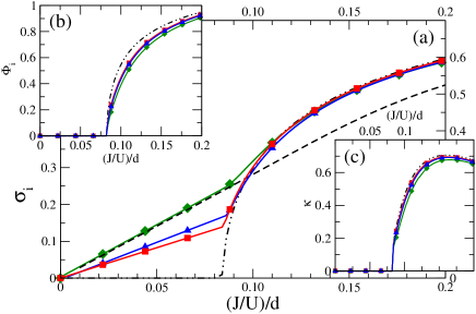
Figure 1: Results from perturbation theory for homogeneous lattices in $d=1$ (diamonds), $d=2$ (triangles), and $d=3$ (squares) dimensions. The dashed-dotted lines in Fig. 1a-c are the Gutzwiller results. (a) Number fluctuations $\sigma_{i}=\sqrt{\langle n_{i}^{2}\rangle-\langle n_{i}\rangle^{2}}$ calculated for a commensurate filling of one boson per lattice site. The dashed line shows the result from the exact diagonalization for 7 lattice sites and $N=7$ bosons. (b) Order parameter $\Phi_{i}=\langle a_{i}\rangle$ and (c) compressibility $\kappa$ both computed at a fixed chemical potential $\mu/U=0.5$.

The leading corrections to the mean values of single lattice-site observables (SLSO) are of second order in $V$. The results for the order parameter $\Phi_{i}$, the compressibility $\kappa$ and the number fluctuations $\sigma_{i}$ are shown in Fig. 1, where the ration $J/U$ has been scaled by the dimension, to keep the same mean-field transition point. The solid lines in Fig. 1 show the results from perturbation theory, as compared to the Gutzwiller result (shown as the dashed - dotted line). All three quantities show a vanishing perturbative correction both for small and large $J/U$, as the Gutzwiller wavefunction becomes a good approximation in these regimes (for lattice dimensions $d>1$). As expected, deviations from the mean-field picture are strongest near the MI-SF transition, where higher-order corrections will become more and more important.

The order parameter $\Phi_{i}=\langle a_{i}\rangle$ shown in Fig. 1b gets suppressed in the SF. Perturbative corrections to the Gutzwiller result are particularly large in 1D (where the order parameter vanishes in reality), but get smaller with increasing dimension. This is not surprising, as Gutzwiller is a mean-field approach and hence a better approximation for higher-dimensional systems. The critical value $(J/U)_{c}$ is not modified within the present perturbative approach.

Figure 1c shows the results for the compressibility

$$\kappa=\frac{M}{N^{2}}\sum_{i=1}^{M}\frac{\partial\langle n_{i}\rangle}{\partial\mu}\,.$$ (9)

The results of perturbation theory (PT) show a decrease of the compressibility, pointing to an increasing stiffness of the SF phase induced by the short-range interaction.

Finally, we computed the local particle number fluctuations $\sigma_{i}=\sqrt{\langle n_{i}^{2}\rangle-\langle n_{i}\rangle^{2}}$. Exact diagonalization calculations have shown that the number fluctuations are changing smoothly at the MI-SF transition Roth01 , whereas the Gutzwiller result predicts vanishing fluctuations in the MI phase, $\sigma_{i}=0$ (see dashed-dotted line in Fig. 1c). Our perturbative results reproduce the non-vanishing part of $\sigma_{i}$ in the MI regime and agree well with our result obtained from exact diagonalization of a one-dimensional system of $7$ lattice sites. Significant deviations from the exact 1D result are seen in the MI-SF transition regions, starting from the mean-field critical value, $(J/U)_{c}=0.086$, up to values of the order of the critical values of $(J/U)_{c}\approx 0.2\cdots 0.3$ usually obtained from DMRG Rapsch01 and QMC Batrouni01 calculations.

Nevertheless, based on the good agreement of our perturbative result with the exact diagonalization for a large region in the MI, we conclude that the number fluctuations are mainly produced by next-neighbor particle-hole fluctuations included in perturbation theory.

IV.2 The Correlation Function

The single-particle density matrix $\rho_{ji}=\langle a_{i}^{\dagger}a_{j}\rangle$ is of particular importance as it describes the correlation between the different lattice sites. The correlation function $\rho_{ij}$ shows off-diagonal long-range order in the SF state (in dimensions $d>1$), in contrast to the MI phase where $\rho_{ij}$ decays exponentially.

The experimental observation Greiner01 of the MI transition relies on the different behavior of the density matrix in the MI and SF regimes, which can be visualized by taking absorption pictures of the freely expanding atomic cloud. Assuming that the expansion time is long enough and that the gas is dilute enough (such that atom-atom interactions can be neglected during the expansion), the shape of the cloud reflects the initial momentum distribution $\rho({\bf k})$, which is directly given by the Fourier-transform of the density matrix $\rho_{ij}$ :

$$\rho({\bf k})=|w({\bf k})|^{2}\sum_{i,j=1}^{M}\rho_{ij}e^{i{\bf k}({\bf r}_{i}-{\bf r}_{j})}\,.$$ (10)

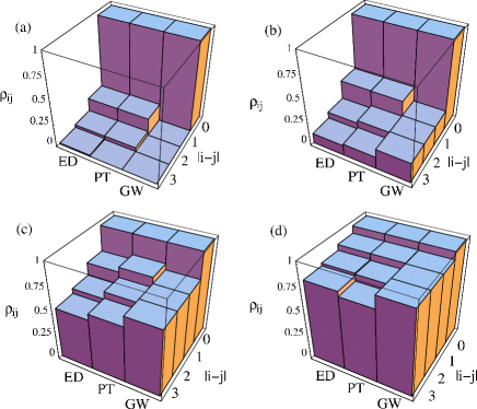
Figure 2: Short-range behavior of the one-particle density matrix $\rho_{ij}$ as a function of site distance $|i-j|$. Results for a homogeneous lattice of 7 sites with $N=7$ Bosons have been obtained from exact diagonalization (ED), from second-order perturbation theory (PT), and from the Gutzwiller mean-field ansatz (GW). (a) $J/U=0.05$ (MI regime), (b) $J/U=0.1$, (c) $J/U=0.2$, (d) $J/U=0.5$ (deep SF regime). All calculations use periodic boundary conditions. The mean-field value $(J/U)_{c}$ for the MI transition in the commensurate case with one boson per lattice site is $(J/U)_{c}=0.086$ in 1D (see Fig. 1). (The MF value differs strongly from $(J/U)_{c}=0.277$ derived from QMC calculations Kuehner01 or $(J/U)_{c}=0.260$ for DMRG calculations Rapsch01 ).

Here, $w({\bf k})$ is the Fourier transform of the Wannier functions $w({\bf r-r}_{i})$ describing the wavefunction of a single lattice site. The presence of the factor $w({\bf k})$ in Eq. (10) provides a cutoff at high momenta.

The mean-field results for $\rho_{ij}$ only describe the different long-range behavior in the MI and SF. For a homogeneous lattice the correlation function calculated from the Gutzwiller wavefunction gives $\rho_{ii}=n_{i}$ for the diagonal elements and then drops instantly to $\rho_{ij}=|\Phi|^{2}$ for all off-diagonal elements $i\neq j$. Short-range correlations are not reproduced by the Gutzwiller approach. This deviation is particularly severe in the MI, where the mean-field result predicts a completely flat momentum distribution, whereas the short-range correlations (i.e. the exponential decay of $\rho_{ij}$) yield smooth bumps in the expansion pattern. These can be distinguished from the $\delta$-peaks of the SF only after a sufficiently long expansion time.

Applying perturbation theory to the GW wavefunction improves the structureless GW correlation function. In Fig. 2, we have compared the results of GW mean-field theory, of PT, and of exact diagonalization (ED). The diagonalization has been carried out for a small 1D lattice, where it is easily feasible. Although there is no long-range order in the SF phase for the 1D case, where the density matrix exhibits a power-law decay towards zero, it is still reasonable to compare the short-range correlations. Indeed, we find a nice agreement between perturbation theory and exact results, not only for the MI (see Fig. 2a), but also for the short-range behavior in the SF. This agreement is made possible by the fact that $\rho_{ij}$ decays only slowly and higher-order corrections show only negligible corrections for small lattices. An example for the SF case is shown in Fig. 2d. However, there is still a considerable difference for $\rho_{i,i+3}$ in Fig. 2d. This is not surprising as we do PT up to second order. Hence correlations over a distance of three and more lattice sites are only corrected by the global mean-field correction for the infinite lattice (see Eq. (22), Eq. (23), and Fig. 8 in Appendix A). We expect better agreement for larger lattice sizes as finite-size effects, arising in small lattices, are still considerable for $M=7$ sites used in our ED calculations.

Finally, for intermediate values of $J/U$, shown in Fig. 2b,c, we observe a faster drop in the off-diagonal correlations, such that higher-order contributions in the PT become more important. In any dimension, the perturbation $V$ is no longer small at the tip of the MI-SF transition lobe (Fig. 2c), and the PT breaks down. Nevertheless, comparing with exact diagonalization results, Fig. 2b shows still good agreement with ED, in contrast to Fig. 2c, which shows clear disagreement. Even though the parameters $J/U=0.2$ chosen for Fig. 2c are close to the MI-SF transition for 1D-lattices (as predicted by DMRG Rapsch01 and QMC Kuehner01 calculations), PT reproduces the correct slope for the off-diagonal decay and lacks only the wrong offset from the mean field. Thus, even for this case, PT represents a qualitative improvement on the Gutzwiller result. The results for both approximations, Gutzwiller and PT, are expected to become better in higher dimensions (with the perturbative corrections diminishing in size).

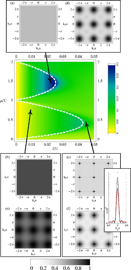
Figure 3: The central figure shows the correction to $\rho_{i,i+1}$ in second-order PT as a function of $\mu/U$ and $J/U$. The order parameter $\langle\phi\rangle$ vanishes inside the Mott-insulating lobes, whose mean-field boundaries are given by the white dashed line. Plots (a) – (f) display the resulting momentum distribution without the Wannier form factor, $\rho({\bf k})/|w({\bf k})|^{2}$, calculated for a 2D lattice with $25\times 25$ lattice sites. (a)-(c) are the Gutzwiller mean-field results, and (d)-(f) are calculated using second-order PT. The inset in (c),(f) shows a cut of one peak taken along $k_{y}a=0$; dashed line for GW and solid line for the PT result. Arrows indicate the position of the respective plots in the $(\mu/U,J/U)$ phase diagram. The parameters used are: $\mu/U=1.5$, $J/U=0.0225$ for (a) and (d); $\mu/U=0.75$, $J/U=0.01$ for (b) and (e); and $\mu/U=0.5$, $J/U=0.044$ for (c) and (f). The gray-scales of plots belonging to the same parameter set are identical. Expansion patterns (a),(b),(d),and (e) are normalized to the peak maximum; (c) and (f) are normalized to $1/20$ of the peak maximum.

As discussed before, the perturbative enhancement of the description of short-range correlations is expected to lead to strong consequences for the momentum distributions. As an example we discuss a set of momentum distributions $\rho({\bf k})/|w({\bf k})|^{2}$ for a homogeneous 2D lattice, Fig. 3a-f, and compare the Gutzwiller results to those improved by PT. The improved PT versions, Figs. 3d-f, show much finer structures than the mean-field results, Fig. 3a-c. PT predicts broad peaks in the MI regions down to very small values of $J/U$, Fig. 3e, whereas the Gutzwiller result without PT shows a structureless flat distribution for the whole MI region, Fig. 3a,b. Naturally, the modifications of $\rho({\bf k})/|w({\bf k})|^{2}$ are strongest near the phase transition, Figs. 3a and 3d.

Going towards larger values $J/U$ into the SF phase, PT gives rise to a suppression of the peaks (inset in Fig. 3c,f). This suppression can be larger than $20\%$ of the original peak height and stems from the corrections to the mean field. Additionally, Fig. 3f shows broad peaks induced by the inclusion of short-range correlations. However, for large lattices, these broad peaks are small compared to the (finite-size broadened) SF $\delta$-peaks.

IV.3 Harmonic Trap Potential

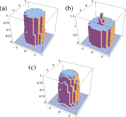
Figure 4: Occupation number $n_{i}$ on a plane through the trap center for a 3D lattice with $15^{3}$ lattice sites. (a) $\mu/U=0.4$, $J/U=0.005$, and $\alpha/U=0.02$. (b) $\mu/U=1.5$, $J/U=0.0075$, and $\alpha/U=0.03$. (c) $\mu/U=0.4$, $J/U=0.0075$, and $\alpha/U=0.02$.

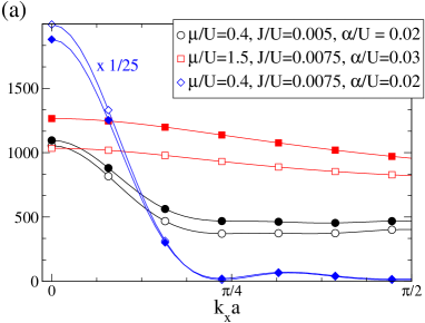
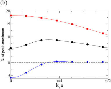
Figure 5: Expansion pattern for a 3D-lattice with $15^{3}$-sites in the presence of a harmonic potential. (a) Momentum distribution without the Wannier form factor, $\rho({\bf k})/|w({\bf k})|^{2}$, calculated along the $k_{x}$ direction. Filled symbols are the PT results and open symbols are the GW results. The graphs for the MI surrounded by a SF shell (diamonds) are rescaled by a factor $1/25$. The results denoted by circles correspond to the occupation distribution of Fig. 4a, diamonds to Fig. 4c, and squares to Fig. 4b. (b) Difference between PT and GW results.

In contrast to what was assumed in the last section, optical lattices used in experiments are not homogeneous. Magnetic or optical trapping potentials are used Pedri01 ; Greiner01 to confine the atomic gas to a finite volume.

The inhomogeneity caused by the trapping potential leads to slowly varying on-site energies, $\epsilon_{i}$, in the Mott-Hubbard model Eq. (1), that can be interpreted as a spatially varying chemical potential $\mu_{\mathrm{local}}=\mu-\epsilon_{i}$. Consequently the lattice is in general not in a pure MI or SF phase, but shows alternating shells of SF and MI regions. An example for a SF region surrounded by a MI shell is shown in Fig. 4b.

Considering the slowly varying on-site energy as a spatially varying chemical potential gives a qualitative understanding of the shell structures. The spatial variation of the chemical potential corresponds to a path parallel to the $\mu/U$ axis in the $\mu/U$-$J/U$-diagram. Starting with the potential minimum, in the trap center, and then moving off the center, decreases the effective local chemical potential. Whenever a MI-SF (SF-MI) phase boundary is hit along the path in the $\mu/U$-$J/U$-diagram, a change from a MI to a SF (SF to MI) shell appears.

The inclusion of short-range correlations gives rise to considerable modifications also in the presence of an inhomogeneous trapping potential. Examples, calculated for a 3D-lattice, are shown in Fig. 5, where an underlying harmonic potential

$$\epsilon_{i}=\alpha\sum_{\beta=1}^{3}i_{\beta}^{2}\,,$$ (11)

was chosen.

The three situations considered here correspond to a case with a large MI fraction (Fig. 4a), a SF island surrounded by a MI shell (Fig. 4b), and a MI island surrounded by a SF phase (Fig. 4c). Calculating the expansion patterns for these situations, Fig. 5, shows that the perturbative corrections arising from the short-range correlations lead to substantially different behavior in the different cases.

For the almost complete MI state we get a correction to all wavevectors $k$, with a fast drop at values close to the peak center $k=0$, which leads to a peak broadening in the expansion picture (see circles in Fig. 5).

Particularly large changes were found for the case of a SF island surrounded by a MI phase, Fig. 5 (squares). Again, corrections arise for all wavevectors, but, in contrast to the almost homogeneous case, the largest increase is now found for $k=0$, with changes of about $20\%$ of the peak-maximum.

Finally, the reversed situation, a MI island surrounded by a SF phase (diamonds in Fig. 5) does not show an increase of its maximum peak height but a considerable reduction (over 5% of the peak maximum). This is not surprising, as the majority of the lattice sites are now contributing to the SF phase, and a peak reduction was also observed for the bulk SF phase.

We would now like to compare our approach with the results obtained by Kashurnikov et al. Kashurnikov01 , who used QMC calculations to calculate expansion patterns for a small 3D lattice with harmonic confinement. There is good qualitative agreement in all cases with high superfluid fraction (compare for example Fig. 6a(b) and Fig. 2b(c) in Ref. Kashurnikov01 ). However, the features of these expansion patterns are already well reproduced using the Gutzwiller mean-field ansatz alone, in particular, the satellite peak, which was discussed as a signature of the MI-SF shell structure in Kashurnikov01 . Corrections arising from PT show a suppression of the SF peak, as was discussed above.

However, there are also considerable discrepancies to the QMC results for situations with a large MI fraction, even after implementing second-order PT. In these cases (Fig. 6c(d) and Fig. 2d(e) in Ref. Kashurnikov01 ), the influence of the MI phase on the expansion picture broadens the peak and leads to a homogeneous background. The discrepancies to the QMC are clearly visible in Fig. 6c showing no peak broadening and a sattelite peak in contrast to the QMC results (Fig.2d in Kashurnikov01 ). Including the short range correlations perturbatively corrects the expansion pattern in the right direction, giving rise to a suppression of the SF-peak. Considering the expansion pattern with the clearest MI features (Fig 6d and Fig. 2e in Ref. Kashurnikov01 ), we obtain the correct peak broadening from GW/PT calculation, but a larger ratio of MI background to SF peak.

Concerning these discrepancies, we note that the expansion pattern is highly sensitive to the value of the mean field. Even small deviations can lead to a change in the SF-peak height sufficient to mask the flat distribution of the MI phase. We checked, however, that the observed discrepancy is not due to a lack in accuracy of our numerical calculations. We therefore believe that the discrepancies between QMC and GW/PT for situations with a large MI fraction can be attributed to the insufficiency of GW and low-order PT in describing the long-range correlations in this inhomogeneous situation. In addition, we note that the lattice employed in Kashurnikov01 is comparatively small for the given harmonic confinement potential (with no complete shell of empty sites at the perimeter, see insets of Fig. 6), i.e., the choice of boundary conditions (periodic in the case of our numerical calculations) may have non-negligible effects on the outer lattice sites.

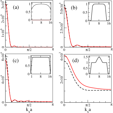
Figure 6: Gutzwiller (dashed line) and perturbation theory (solid line) expansion patterns (cuts along $k_{x}$) for a system of $16^{3}$ lattice sites considered in Kashurnikov01 . All plots are without the Wannier form factor, $\rho({\bf{k}})/|w({\bf k})|^{2}$. The insets show the occupation number $n_{i}$ for a cut along the $\hat{x}$-direction. (a) $J/U=1/32$, $\mu=0.3775$, $\alpha=0.00610$. (b) $J/U=1/80$, $\mu=0.3125$, $\alpha=0.01221$. (c) $J/U=1/80$, $\mu=0.625$, $\alpha=0.01288$. (d) $J/U=1/80$, $\mu=1$, $\alpha=0.02505$. (Note however, that the Hamiltonian used in Kashurnikov01 differs from Eq. (1) and hence the parameters are converted to the corresponding quantities used in our definitions.)

V Conclusions

We have used perturbation theory to incorporate the effects of short-range correlations on top of the mean field solution of the bosonic Mott Hubbard model. We derived corrections to local quantities, as well as to observable expansion patterns. We numerically calculated the corrections to the MF-result, using PT up to second order, thus including correlations between next and next-nearest lattice sites. Modifications to the particle number fluctuations $\sigma_{i}$, arising from the PT, gave rise to the expected smooth transition of $\sigma_{i}$ at the MI-SF transition. Moreover, comparing the PT results to the ED results for $\sigma_{i}$ in 1D lattices showed good agreement for small values of $J/U$. Of particular importance are the corrections to the correlation function, and thus to the expansion patterns. We compared the correlation function obtained from PT with calculations from ED for small 1D-lattices and found good agreement. Studying the expansion patterns showed that the inclusion of the short-range correlations to the MF-ansatz gives rise to distinct modifications. A broad peak can be seen in the PT results for the MI regime, visible even down to small values of $J/U$. Comparing PT and MF expansion patterns obtained for parameters in the SF region displayed a considerable suppression of the SF peak in the PT results. Additionally, on approaching the SF-MI transition from the SF side, broad peaks underlying the SF peaks were found in the PT-expansion patterns. Including a harmonic confinement potential leads to situations where SF and MI regions coexist. Hence the perturbative corrections to the expansion pattern become more complex. We studied lattices with different underlying harmonic traps giving rise to different constellations of SF-MI regions, finding modifications of up to $20\%$ of the peak maximum in the expansion patterns.

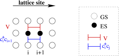
Figure 7: Schematic diagram illustrating the term $\langle c_{i}^{\dagger}c_{j}\frac{1}{\Delta}V_{ij}\rangle_{0}$ appearing in the first-order correction ${\langle c_{i}^{\dagger}c_{j}\rangle}_{1}$ of the density matrix, where $V_{ij}=\frac{J}{2}(c_{i}^{\dagger}c_{j}+c_{j}^{\dagger}c_{i})$ is the perturbation connecting sites $i$ and $j$. The diagram shows the lattice sites in the horizontal direction. The different steps needed to obtain the matrix element are shown vertically. Open circles denote the ground state (GS) of the given lattice site, while filled circles are excited states (ES) of this site, for the mean-field Hamiltonian $H_{\mathrm{MF}}$.

Appendix A Derivation of the Matrix Elements

We use standard stationary perturbation theory tannoudji01 to calculate the corrections to the mean-field results induced by the perturbation

$$V=-\sum_{\langle i,j\rangle}V_{ij}=-\frac{J}{2}\sum_{\langle i,j\rangle}(c_{i}^{\dagger}c_{j}+c_{j}^{\dagger}c_{i})\,,$$ (12)

where we introduce the new operators

$$c_{i}=a_{i}-\langle a_{i}\rangle_{0}=a_{i}-\Psi_{i}\,,$$ (13)

The expectation value $\langle\cdot\rangle_{0}$ is taken with respect to the MF wavefunction $|G_{0}\rangle$. Defining the operator for the energy denominator as

$$\frac{1}{\Delta}\equiv\frac{1-|G_{0}\rangle\langle G_{0}|}{\epsilon_{0}-H_{\mathrm{MF}}}\,,$$ (14)

the expectation value of an observable $\langle A\rangle$ including all corrections up to second order is

$$\begin{split}\langle A\rangle\approx&\langle A\rangle_{0}+\langle V\frac{1}{\Delta}A\rangle_{0}+\langle A\frac{1}{\Delta}V\rangle_{0}\\ &+\langle V\frac{1}{\Delta}V\frac{1}{\Delta}A\rangle_{0}+\langle V\frac{1}{\Delta}A\frac{1}{\Delta}V\rangle_{0}\\ &+\langle A\frac{1}{\Delta}V\frac{1}{\Delta}V\rangle_{0}-\langle V\frac{1}{\Delta^{2}}V\rangle_{0}\langle A\rangle_{0}\,.\end{split}$$ (15)

The first line in Eq. (15) is the MF-result $\langle A\rangle_{0}$, followed by two contributions which are the first-order corrections. Lines two and three in Eq. (15) are the second-order corrections to the mean value.

A.1 Density Matrix: First-Order Corrections

As an example we will discuss the corrections to the density matrix $\rho_{ij}=\langle a_{i}^{\dagger}a_{j}\rangle$. The first-order correction to the density matrix is:

$$\langle a_{i}^{\dagger}a_{j}\rangle_{1}=\langle c_{i}^{\dagger}c_{j}\rangle_{1}+\Psi_{i}^{*}\langle c_{j}\rangle_{1}+\langle c_{i}^{\dagger}\rangle_{1}\Psi_{j}+\Psi_{i}^{*}\Psi_{j}\,.$$ (16)

For two different lattice sites $i\neq j$, we find

$$\langle c_{i}^{\dagger}c_{j}\frac{1}{\Delta}c_{i}\rangle_{0}=\langle c_{j}\rangle_{0}\langle c_{i}^{\dagger}\frac{1}{\Delta}c_{i}\rangle_{0}=0\,,$$ (17)

since the Gutzwiller ground state is a product state. As a consequence, the contributions $\langle c_{i}^{\dagger}\rangle_{1}$ and $\langle c_{j}\rangle_{1}$ vanish. The only remaining contributions to $\langle a_{i}^{\dagger}a_{j}\rangle_{1}$ stem from

$$\langle c_{i}^{\dagger}c_{j}\rangle_{1}=-\langle V_{ij}\frac{1}{\Delta}c_{i}^{\dagger}c_{j}\rangle_{0}-\langle c_{i}^{\dagger}c_{j}\frac{1}{\Delta}V_{ij}\rangle_{0}\,,$$ (18)

and $\Psi_{i}^{*}\Psi_{j}$.

To get a better idea of the character of the terms arising in the perturbative expansion, we introduce, in Fig. 7, a graphical representation (for the example of a 1D-lattice).

The graph shows a decomposition of the matrix element, with each row showing the wavefunction at an intermediate step in the evaluation of the matrix element. As we deal with product states

$$|G^{\alpha}\rangle=\prod_{i=1}^{M}|i_{\alpha_{i}}\rangle\,,$$ (19)

we represent the wavefunction by a row of circles, where each circle denotes the state $|i_{\alpha_{i}}\rangle$ of a particular lattice site $i$.

Open circles in Fig. 7 denote a lattice site in its ground state (GS), filled circles refer to an excited state (ES) of this particular lattice site, with respect to the local mean-field Hamiltonian. Note that, in general, this can be an arbitrarily highly excited state (although higher contributions are suppressed by the energy denominator, and a cutoff is used in practice).

Starting with a row of open circles, denoting the GS, $|G_{0}\rangle$, each following row corresponds to the state after the action of $V$ or $c_{i}^{\dagger}c_{j}$, as indicated on the left side of the graph. As all matrix elements in Eq. (15) can be expressed in terms of a GS expectation value $\langle\cdot\rangle_{0}$ and a sequence of $V$ and $c_{i}^{\dagger}c_{j}$ operators, the first and last row must always be a line of open circles.

Let us consider for instance the second term in Eq. (18)

$$\langle c_{i}^{\dagger}c_{j}\frac{1}{\Delta}V_{ij}\rangle_{0}\,.$$ (20)

Reading the graph in Fig. 7 from top to bottom corresponds to reading the matrix element from right to left. Starting with the GS, $|G_{0}\rangle$, the first row consists of open circles. The second row shows the state after the action of the perturbation $V$. Acting with $V_{ij}$ to the right onto the GS results in a state

$$V_{ij}|G_{0}\rangle=\sum_{\alpha,\beta}f_{\alpha,\beta}|i_{\alpha},j_{\beta}\rangle\,,$$ (21)

where $i$ and $j$ are neighboring lattice sites and $|i_{\alpha},j_{\beta}\rangle$ denotes the state with lattice site $i$ ($j$) in the exited state $\alpha$ ($\beta$) and all other sites in their GS. Thus the second row shows the lattice sites $i$ and $i+1$ in an excited state (filled circle), as the perturbation, Eq. (12), allows only next neighbor interactions. Finally, the action of $c_{i}^{\dagger}c_{j}$ has to bring the excited states back to the GS, in order to get a non-vanishing contribution. Therefore, in first order PT, only next neighbor corrections to the correlation function arise, as the final row must represent the ground state $\langle G_{0}|$ again. The graph representing the remaining first term in Eq. (18) is obtained by rotating the graph in Fig. 7 by $\pi$.

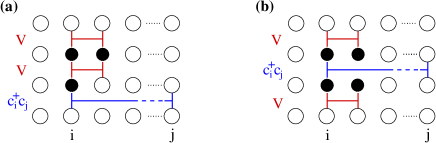
Figure 8: Diagrammatic representation of the contributions from $\Psi_{i}^{*}\langle c_{j}\rangle_{2}$ and $\langle c_{i}^{\dagger}\rangle_{2}\Psi_{j}$ to the second-order correction of the density matrix. (a) Terms representing contributions of the form Eq. (22). (b) contributions of the form Eq. (23). All notations are the same as in Fig. 7.

A.2 Density Matrix: Second-Order Corrections

Rewriting the second-order corrections to the density matrix, $\langle a_{i}^{\dagger}a_{j}\rangle_{2}$, in terms of the operators $c_{i}^{\dagger}$ and $c_{j}$ gives Eq. (16), but with $\langle\cdot\rangle_{1}$ replaced by $\langle\cdot\rangle_{2}$. In contrast to the first-order corrections, now the terms proportional to $\langle c_{j}\rangle_{2}$ and $\langle c_{i}^{\dagger}\rangle_{2}$ also give non-vanishing contributions. Using Eq. (15) we obtain:

$$\langle c_{j}\rangle_{2} =\sum_{k}^{\prime}\langle V_{jk}\frac{1}{\Delta}V_{jk}\frac{1}{\Delta}c_{j}\rangle_{0}+\sum_{k}^{\prime}\langle c_{j}\frac{1}{\Delta}V_{jk}\frac{1}{\Delta}V_{jk}\rangle_{0}$$ (22)

$$+\sum_{k}^{\prime}\langle V_{jk}\frac{1}{\Delta}c_{j}\frac{1}{\Delta}V_{jk}\rangle_{0}\,.$$ (23)

Here, the primed sums run over all neighbors $k$ to site $j$. The corresponding subset of graphs for $\Psi_{i}^{*}\langle c_{j}\rangle_{2}$ and $\langle c_{i}^{\dagger}\rangle_{2}\Psi_{j}$ are given by Fig. 8a and Fig. 8b for Eq. (22) and Eq. (23) respectively. Note that all terms of Eq. (22) and Eq. (23) give a correction to all matrix elements of the density matrix independent of the distance between the lattice sites. We can understand these contributions as a modification to the MF value of the density matrix.

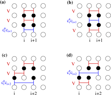
Figure 9: Graphs showing second-order corrections arising from $\langle c_{i}^{\dagger}c_{j}\rangle_{2}$. Diagrams (a) and (b) are coming from direct-neighbor contributions as given by Eq. (24) and Eq. (25) respectively. Diagrams (c) and (d) are next-nearest-neighbor contributions: (c) corresponds to Eq. (27) and Eq. (28); (d) corresponds to Eq. (29).

For the second-order contribution, $\langle c_{i}^{\dagger}c_{j}\rangle_{2}$, we have to distinguish two cases:

• Lattice site $i$ and $j$ being direct neighbors. In this case we get

  $$\langle c_{i}^{\dagger}c_{j}\rangle_{2}= \langle V_{ij}\frac{1}{\Delta}V_{ij}\frac{1}{\Delta}c_{i}^{\dagger}c_{j}\rangle_{0}+\langle c_{i}^{\dagger}c_{j}\frac{1}{\Delta}V_{ij}\frac{1}{\Delta}V_{ij}\rangle_{0}$$ (24)

  $$+\langle V_{ij}\frac{1}{\Delta}c_{i}^{\dagger}c_{j}\frac{1}{\Delta}V_{ij}\rangle_{0}\,.$$ (25)

  Corrections for Eq. (24) and Eq. (25) are shown in Fig. 9a and Fig. 9b, respectively.

• Configurations corresponding to two lattice sites $i\neq j$ connected by two successive hopping steps via site $k$. This gives rise to six contributions:

  $$\langle c_{i}^{\dagger}c_{j}\rangle_{2}=\qquad$$ (26)

  $$\sum_{\mathcal{C}}\langle V_{jk}\frac{1}{\Delta}V_{ki}\frac{1}{\Delta}c_{i}^{\dagger}c_{j}\rangle_{0}+\sum_{\mathcal{C}}\langle V_{ki}\frac{1}{\Delta}V_{jk}\frac{1}{\Delta}c_{i}^{\dagger}c_{j}\rangle_{0}\qquad$$ (27)

  $$+\sum_{\mathcal{C}}\langle c_{i}^{\dagger}c_{j}\frac{1}{\Delta}V_{jk}\frac{1}{\Delta}V_{ki}\rangle_{0}+\sum_{\mathcal{C}}\langle c_{i}^{\dagger}c_{j}\frac{1}{\Delta}V_{ki}\frac{1}{\Delta}V_{jk}\rangle_{0}\qquad$$ (28)

  $$+\sum_{\mathcal{C}}\langle V_{jk}\frac{1}{\Delta}c_{i}^{\dagger}c_{j}\frac{1}{\Delta}V_{ki}\rangle_{0}+\sum_{\mathcal{C}}\langle V_{ki}\frac{1}{\Delta}c_{i}^{\dagger}c_{j}\frac{1}{\Delta}V_{jk}\rangle_{0}\,.\qquad$$ (29)

  An example for the contributions arising from Eq. (27) and Eq. (28) is shown in Fig. 9c. The last term, Eq. (29), has the representation shown in Fig. 9d. Note that for lattices with dimensions $d>1$, the sites $i$,$j$ and $k$ need not necessarily form a straight line but can form a chevron.

References

- (1) M. P. A. Fisher, P. B. Weichman, G. Grinstein, and D. S. Fisher, Phys. Rev. B 40, 546 (1989).
- (2) D. Jaksch, C. Bruder, J. I. Cirac, C. W. Gardiner, and P. Zoller, Phys. Rev. Lett. 81, 3108 (1998).
- (3) M. Greiner, O. Mandel, T. Esslinger, T. W. Hänsch, and I. Bloch, Nature (London) 415, 39 (2002).
- (4) D. Jaksch, H.-J. Briegel, J. I. Cirac, C. W. Gardiner, and P. Zoller, Phys. Rev. Lett. 82, 1975 (1999).
- (5) D. Jaksch, V. Venturi, J. I. Cirac, C. J. Williams, and P. Zoller, Phys. Rev. Lett. 89, 040402 (2002).
- (6) W. Hofstetter, J. I. Cirac, P. Zoller, E. Demler, and M. D. Lukin, Phys. Rev. Lett. 89, 220407 (2002).
- (7) E. Altman and A. Auerbach, Phys. Rev. Lett. 89, 250404 (2002).
- (8) W. Zwerger, J. Opt. B: Quantum Semiclass. Opt. 5, S9 (2003).
- (9) H. P. Büchler, G. Blatter, and W. Zwerger, Phys. Rev. Lett. 90, 130401 (2003).
- (10) D. C. Roberts and K. Burnett, Phys. Rev. Lett. 90, 150401 (2003).
- (11) H. Kleinert, S. Schmidt, and A. Pelster, cond-mat/0307412.
- (12) B. Damski, J. Zakrzewski, L. Santos, P. Zoller, and M. Lewenstein, Phys. Rev. Lett. 91, 080403 (2003).
- (13) P. Rabl, A. J. Daley, P. O. Fedichev, J. I. Cirac, and P. Zoller, Phys. Rev. Lett. 91, 110403 (2003).
- (14) H. P. Büchler and G. Blatter, Phys. Rev. Lett. 91, 130404 (2003).
- (15) M. Lewenstein, L. Santos, M. A. Baranov, and H. Fehrmann, Phys. Rev. Lett. 92, 050401 (2004)
- (16) M. Greiner, O. Mandel, T. W. Hänsch, and I. Bloch, Nature (London) 419, 51 (2002).
- (17) O. Mandel, M. Greiner, A. Widera, T. Rom, T. W. Hänsch, and I. Bloch, Nature (London) 425, 937 (2003).
- (18) T. Stöferle, H. Moritz, C. Schori, M. Köhl, and T. Esslinger, Phys. Rev. Lett. 92, 130403 (2004).
- (19) H.-J. Briegel and R. Raussendorf, Phys. Rev. Lett. 86, 910 (2001).
- (20) J. K. Freericks and H. Monien, Phys. Rev. B 53, 2691 (1996).
- (21) D. van Oosten, P. van der Straten, and H. T. C. Stoof, Phys. Rev. A 63, 053601 (2001).
- (22) A. M. Rey, K. Burnett, R. Roth, M. Edwards, C. J. Williams, and C. W. Clark, J. Phys. B 36, 825 (2003).
- (23) D. S. Rokhsar and B. G. Kotliar, Phys. Rev. B 44, 10328 (1991).
- (24) T. D. Kühner and H. Monien, Phys. Rev. B 58, R14741 (1998).
- (25) S. Rapsch, U. Schollwöck, and W. Zwerger, Europhys. Lett. 46, 559 (1999).
- (26) C. Kollath, U. Schollwöck, J. von Delft, and W. Zwerger, Phys. Rev. A 69, 031601 (2004).
- (27) R. Roth and K. Burnett, Phys. Rev. A 68, 023604 (2003).
- (28) R. Roth and K. Burnett, Phys. Rev. A 67, 031602(R) (2003).
- (29) R. T. Scalettar, G. G. Batrouni, and G. T. Zimanyi, Phys. Rev. Lett. 66, 3144 (1991).
- (30) G. G. Batrouni and R. T. Scalettar, Phys. Rev. B 46, 9051 (1992).
- (31) W. Krauth and N. Trivedi, Europhys. Lett. 14, 627 (1991); W. Krauth, N. Trivedi and D. Ceperley, Phys. Rev. Lett. 67, 2307 (1991).
- (32) J. Kisker and H. Rieger, Phys. Rev. B 55, R11981 (1996).
- (33) V. A. Kashurnikov, N. V. Prokof’ev, and B. V. Svistunov, Phys. Rev. A 66, 031601(R) (2002).
- (34) N. Elstner and H. Monien, cond-mat/9905367 (unpublished).
- (35) K. Sheshadri, H. R. Krishnamurthy, R. Pandit, and T. V. Ramakrishnan, Europhys. Lett. 22, 257 (1993).
- (36) P. Pedri et al., Phys. Rev. Lett. 87, 220401 (2001).
- (37) C. Cohen-Tannoudji, B. Diu, and F. Laloë, Quantum Mechanics (Hermann, Paris, 1977).