Probing microcavity polariton superfluidity through resonant Rayleigh scattering

Abstract

We investigate the two-dimensional motion of polaritons injected into a planar microcavity by a continuous wave optical pump in presence of a static perturbation, e.g. a point defect. By finding the stationary solutions of the nonlinear mean-field equations (away from any parametric instability), we show how the spectrum of the polariton Bogoliubov-like excitations reflects onto the shape and intensity of the resonant Rayleigh scattering emission pattern in both momentum and real space. We find a superfluid regime in the sense of the Landau criterion, in which the Rayleigh scattering ring in momentum space collapses as well as its normalized intensity. More generally, we show how collective excitation spectra having no analog in equilibrium systems can be observed by tuning the excitation angle and frequency. Predictions with realistic semiconductor microcavity parameters are given.

The concept of a quantum fluid has played a central role in many fields of condensed matter and atomic physics, ranging from superconductors to Helium fluids ManyBody and, more recently, atomic Bose-Einstein condensates AtomicBEC . One of the most exciting manifestations of quantum behavior is superfluidity, i.e. the possibility of the fluid to flow without friction around an impurity Superfluidity .

In this Letter, we investigate the superfluid properties of a two-dimensional gas of polaritons in a semiconductor microcavity in the strong light-matter coupling regime Weisbuch . In this system, the normal modes are superpositions of a cavity photon and a quantum well exciton. Thanks to their photonic component, polaritons can be coherently excited by an incident laser field and detected through angularly or spatially resolved optical spectroscopy. Thanks to their excitonic component, polaritons have strong binary interactions, which have been demonstrated to produce spectacular polariton amplification effects Savvidis ; Saba through matter-wave stimulated collisions Ciuti , as well as spontaneous parametric instabilities Baumberg ; Messin ; Review .

Here, we study the propagation of a polariton fluid in presence of static imperfections, which are known to produce resonant Rayleigh scattering (RRS) of the exciting laser field RRS ; HoudreRRSLin ; HoudreRRSNLin ; Langbein_ring . We show that superfluidity of the polariton fluid manifests itself as a quenching of the RRS intensity when the flow velocity imprinted by the exciting laser is slower than the sound velocity in the polariton fluid. Furthermore, a dramatic reshaping of the RRS pattern due to polariton-polariton interactions can be observed in both momentum and real space even at higher flow velocities. Interestingly, the polariton field oscillation frequency is not fixed by an equation of state relating the chemical potential to the particle density, but it can be tuned by the frequency of the exciting laser. This opens the possibility of having a spectrum of collective excitation around the stationary state which has no analog in usual systems close to thermal equilibrium. We show in detail how these peculiar excitation spectra can be probed by resonant Rayleigh scattering.

A commonly used model for describing a planar microcavity containing a quantum well with an excitonic resonance strongly coupled to a cavity mode is based on the Hamiltonian Ciuti_Review :

$${\mathcal{H}}=\int\!d{\bf x}\,\sum_{ij=\{X,C\}}\hat{\Psi}^{\dagger}_{i}({\bf x})\,\Big{[}{\mathbf{h}}^{0}_{ij}+V_{i}({\bf x})\,\delta_{ij}\Big{]}\,\hat{\Psi}_{j}({\bf x})\\ +\frac{\hbar g}{2}\int\!d{\bf x}\,\hat{\Psi}^{\dagger}_{X}({\bf x})\,\hat{\Psi}^{\dagger}_{X}({\bf x})\,\hat{\Psi}_{X}({\bf x})\,\hat{\Psi}_{X}({\bf x})+\\ +\int\!d{\bf x}\,\hbar F_{p}\,e^{i({\bf k}_{p}{\bf x}-\omega_{p}t)}\,\hat{\Psi}^{\dagger}_{C}({\bf x})+\textrm{h.c.}~{},$$ (1)

where ${\bf x}$ is the in-plane spatial position and the field operators $\Psi_{X,C}({\bf x})$ respectively describe excitons ($X$) and cavity photons ($C$). They satisfy Bose commutation rules, $[\hat{\Psi}_{i}({\bf x}),\hat{\Psi}^{\dagger}_{j}({\bf x}^{\prime})]=\delta^{2}({\bf x}-{\bf x}^{\prime})\,\delta_{ij}$. The linear Hamiltonian ${\mathbf{h}}^{0}$ is:

$${\mathbf{h}}^{0}=\hbar\left(\begin{array}[]{cc}\omega_{X}(-i\nabla)&\Omega_{R}\\ \Omega_{R}&\omega_{C}(-i\nabla)\end{array}\right),$$ (2)

where $\omega_{C}({\bf k})=\omega_{C}^{0}\,\sqrt{1+{{\bf k}^{2}}/{k_{z}^{2}}}$ is the cavity dispersion as a function of the in-plane wavevector ${\bf k}$ and $k_{z}$ is the quantized photon wavevector in the growth direction. $\Omega_{R}$ is the Rabi frequency of the exciton-cavity photon coupling. A flat exciton dispersion $\omega_{X}({\bf k})=\omega_{X}$ will be assumed in the following. In this framework, polaritons simply arise as the eigenmodes of the linear Hamiltonian (2); $\omega_{LP(UP)}({\bf k})$ denotes the dispersion of the lower (upper) polariton branch [Fig.1(a)].

The external force term proportional to $F_{p}$ describes a coherent and monochromatic laser field of frequency $\omega_{p}$ (called the pump), which drives the cavity and injects polaritons. Spatially, it is assumed to have a plane-wave profile of wavevector $k_{p}=\sin\theta_{p}\;\omega_{p}/c$, $\theta_{p}$ being the pump incidence angle, so to generate a polariton fluid with a non-zero flow velocity along the cavity plane. The nonlinear interaction term is due exciton-exciton collisional interactions and, as usual, is modelled by a repulsive ($g>0$) contact potential. The anharmonic exciton-photon coupling has a negligible effect in the regime considered in the present study Ciuti_Review . $V_{X,C}({\bf x})$ are external potential terms acting on the excitonic and photonic fields which can model the presence of disorder. Here, results for the specific case of a point defect will be presented. Note that point defects can be naturally present in state-of-the-art samples Langbein or even be created deliberately by means of lithographic techniques.

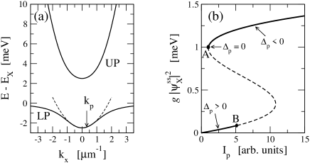
Figure 1: (a): linear dispersion of the lower (LP) and upper (UP) polariton branches. Typical position of the pump wavevector ${\bf k}_{p}$ (arrow), well in the parabolic region of the LP dispersion; the dashed line is the parabolic approximation at small ${\bf k}$. (b): internal vs. incident intensity curve showing bistable behavior. The dashed branch is unstable: the inversion points $A$ and $B$ are respectively due to a single-mode (Kerr) or a multi-mode (parametric) instability. Excitation parameters: $k_{p}=0.314\,\mu\textrm{m}^{-1}$, $\omega_{p}-\omega_{LP}({\bf k}_{p})=0.47\,\textrm{meV}$. Cavity parameters are taken from ref.HoudreRRSLin : $\gamma=0.1\,\textrm{meV}$, $\omega_{X}=\omega_{C}^{0}=1.4\,\textrm{eV}$, $2\,\Omega_{R}=5\,\textrm{meV}$.

Within the mean-field approximation, the time-evolution of the mean fields $\psi_{X,C}({\bf x})=\langle\hat{\Psi}_{X,C}({\bf x})\rangle$ under the Hamiltonian (1) is given by:

$$i\,\frac{d}{dt}\left(\begin{array}[]{c}\psi_{X}({\bf x})\\ \psi_{C}({\bf x})\end{array}\right)=\left(\begin{array}[]{c}0\\ F_{p}\,e^{i({\bf k}_{p}{\bf x}-\omega_{p}t)}\end{array}\right)+\left[{\mathbf{h}}^{0}-\frac{i\gamma}{2}\,{\mathbf{1}}+\right.\\ +\left.\left(\begin{array}[]{cc}V_{X}({\bf x})+g|\psi_{X}({\bf x})|^{2}&0\\ 0&V_{C}({\bf x})\end{array}\right)\right]\left(\begin{array}[]{c}\psi_{X}({\bf x})\\ \psi_{C}({\bf x})\end{array}\right).$$ (3)

In the quantum fluid language, these are the Gross-Pitaevskii equations AtomicBEC for our cavity-polariton system. For simplicity, an equal rate $\gamma$ is assumed for the damping of both the excitonic and the photonic fields. In the present work, we will be concerned with an excitation close to the bottom of the LP dispersion, i.e. the region most protected Review from the exciton reservoir, which may be responsible for excitation-induced decoherence savasta .

In the homogeneous case ($V_{X,C}=0$), we can look for spatially homogeneous stationary states of the system in which the field has the same plane wave structure $\psi_{X,C}({\bf x},t)=\exp[i({\bf k}_{p}{\bf x}-\omega_{p}t)]\,\psi^{ss}_{X,C}$ as the incident laser field. The resulting equations

$$\Big{(}\omega_{X}({\bf k}_{p})-\omega_{p}-\frac{i}{2}\gamma+g\,|\psi_{X}^{ss}|^{2}\Big{)}\,\psi^{ss}_{X}+\Omega_{R}\,\psi_{C}^{ss}=0$$ (4)

$$\Big{(}\omega_{C}({\bf k}_{p})-\omega_{p}-\frac{i}{2}\gamma\Big{)}\,\psi^{ss}_{C}+\Omega_{R}\,\psi_{X}^{ss}=-F_{p},$$ (5)

are the generalization of the state equation. While the oscillation frequency of the condensate wavefunction in an isolated gas is equal to the chemical potential $\mu$ and therefore it is fixed by the equation of state, in the present driven-dissipative system it is equal to the frequency $\omega_{p}$ of the driving laser and therefore it is an experimentally tunable parameter. As usual, stability of the solutions of Eqs. (4-5) has to be checked by linearizing Eq. (3) around the stationary state. For $\omega_{p}>\omega_{LP}({\bf k}_{p})$, the relation between the incident intensity $I_{p}\propto|F_{p}|^{2}$ and the internal one shows the typical S-shape of optical bistability (see Fig.1b and Refs.BistableExp ; BistableExp2 ; Bistability ). Note that nice hysteresis loops due to polariton bistability have been recently experimentally demonstrated BistableExp in the case ${\bf k}_{p}=0$. In the opposite case $\omega_{p}<\omega_{LP}({\bf k}_{p})$ (not shown), the behaviour of the system would instead be the typical one of an optical limiter Bistability .

In the stability region, the response of the system to a weak perturbation can be determined by means of the linearized theory. In the field of quantum fluids, this approach is called Bogoliubov theory AtomicBEC . By defining the slowly varying fields with respect to the pump frequency as $\delta\phi_{i}({\bf x},t)=\delta{\psi_{i}}({\bf x},t)\exp(i\omega_{p}t)$, the motion equation of the four-component displacement vector $\delta{\vec{\phi}}({\bf x},t)=\big{(}\delta\phi_{X}({\bf x},t),\delta\phi_{C}({\bf x},t),\delta\phi^{*}_{X}({\bf x},t),\delta\phi_{C}^{*}({\bf x},t)\big{)}^{T}$ reads

$$i\frac{d}{dt}\delta{\vec{\phi}}={\mathcal{L}}\cdot\delta{\vec{\phi}}+{\vec{f}}_{d}~{},$$ (6)

${\vec{f}}_{d}$ being the source term due to the weak perturbation and the spectral operator ${\mathcal{L}}$ being defined as

$${\mathcal{L}}=\left(\begin{array}[]{cccc}\omega_{X}+2g\,|\psi_{X}^{ss}|^{2}-\omega_{p}-\frac{i\gamma}{2}&\Omega_{R}&g\,\psi^{ss\,2}_{X}\,e^{2i{\bf k}_{p}{\bf x}}&0\\ \Omega_{R}&\omega_{C}(-i\nabla)-\omega_{p}-\frac{i\gamma}{2}&0&0\\ -g\,\psi^{ss\,*\,2}_{X}\,e^{-2i{\bf k}_{p}{\bf x}}&0&-\big{(}\omega_{X}+2g\,|\psi_{X}^{ss}|^{2}\big{)}+\omega_{p}-\frac{i\gamma}{2}&-\Omega_{R}\\ 0&0&-\Omega_{R}&-\omega_{C}(-i\nabla)+\omega_{p}-\frac{i\gamma}{2}\end{array}\right).$$ (7)

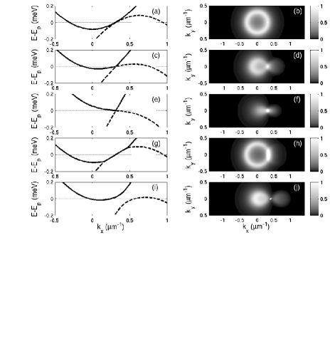
Figure 2: Left panels: exact Bogoliubov dispersion for the LP branches calculated from Eq.(7). Right panels: corresponding RRS emission pattern in ${\bf k}$-space. The intensity has been normalized to the transmitted intensity. The ${\bf k}_{p}$ point (indicated by a white circle) saturates by far the gray scale. Panels (a-f): resonant case $\Delta_{p}=0$ respectively in the linear regime (a-b), with $g|\Psi^{ss}_{X}|^{2}=0.2\,\textrm{meV}$ (c-d), $1\,\textrm{meV}$ (e-f). Panels (g-h): $\Delta_{p}>0$ case with $g|\Psi^{ss}_{X}|^{2}=0.04\,\textrm{meV}$. Panels (i-j): $\Delta_{p}<0$ case with $g|\Psi^{ss}_{X}|^{2}=0.6\,\textrm{meV}$. Pump wavevector: $k_{p}=0.314\,\mu\textrm{m}^{-1}$ (a-h), $0.408\,\mu\textrm{m}^{-1}$ (i-j). Same cavity parameters as in Fig.1.

The eigenvalues of the operator ${\mathcal{L}}$ correspond to the frequencies of the Bogoliubov eigenmodes of the system. For each ${\bf k}$, the spectrum is composed of four branches $\omega^{\pm}_{UP,LP}({\bf k})$: for each polariton branch (LP or UP), two $\pm$ branches exist, which are the image of each other under the simultaneous transformations ${\bf k}\rightarrow 2{\bf k}_{p}-{\bf k}$ and $\omega\rightarrow 2\omega_{p}-\omega$ Ciuti_PL . Numerical calculations are shown in Fig.2. For the sake of clarity, only the branches relative to the LP have been traced, the ones relative to the UP being far away on the scale of the figure. These numerical results can be understood through the simplified analytical approximation that follows.

Provided the interaction energy $g\,|\psi_{X}^{ss}|^{2}$ is much smaller than the polaritonic splitting $\omega_{UP}-\omega_{LP}$, there is no significant mixing between the LP and UP branches. Since we are interested in nearly-resonant excitation close to the bottom of the LP dispersion curve, we can describe the system in terms of the LP field $\psi_{LP}=X_{LP}\psi_{X}+C_{LP}\psi_{C}$ only, being $X_{LP}$ and $C_{LP}$ the Hopfield coefficients quantifying the excitonic and photonic components. In the parabolic approximation, $\omega_{LP}({\bf k})\simeq\omega_{LP}^{0}+\hbar\,{\bf k}^{2}/2m_{LP}$ and the self-coupling constant is $g_{LP}=g\,|X_{LP}|^{4}$. The mean-field shift of the polariton mode is then $\delta\omega_{MF}=g_{LP}\,|\psi_{LP}^{ss}|^{2}$. Under these assumptions, the spectrum of the LP Bogoliubov excitations can be approximated by the simple expression

$$\omega^{\pm}_{LP}\simeq\omega_{p}+\delta{\bf k}\cdot{\bf v}_{p}-\frac{i\gamma}{2}\pm\sqrt{(2\,\delta\omega_{MF}+\eta_{\delta{\bf k}}-\Delta_{p})(\eta_{\delta{\bf k}}-\Delta_{p})},$$ (8)

where $\delta{\bf k}={\bf k}-{\bf k}_{p}$, $\eta_{\delta{\bf k}}=\hbar\,\delta{\bf k}^{2}/2m_{LP}$, the flow velocity ${\bf v}_{p}=\hbar{\bf k}_{p}/m_{LP}$, and the effective pump detuning

$$\Delta_{p}=\omega_{p}-\omega_{LP}({\bf k}_{p})-\delta\omega_{MF}.$$ (9)

In the resonant case ($\Delta_{p}=0$), the $\pm$ branches touch at ${\bf k}={\bf k}_{p}$. The effect of the finite flow velocity ${\bf v}_{p}$ is to tilt the standard Bogoliubov dispersion AtomicBEC via the term $\delta{\bf k}\cdot{\bf v}_{p}$. While in the non-interacting case in Fig.2(a) the dispersion remains parabolic, in the presence of interactions [Fig.2(c) and (e)] its slope has a discontinuity at ${\bf k}={\bf k}_{p}$: on each side of the corner, the $+$ branch starts linearly with group velocities respectively given by $v_{g}^{r,l}=c_{s}\pm v_{p}$, $c_{s}$ being the usual sound velocity of the interacting Bose gas $c_{s}=\sqrt{\hbar\,\delta\omega_{MF}/m_{LP}}$. On the hysteresis curve of Fig.1(b), the condition $\Delta_{p}=0$ corresponds to the inversion point $A$. If one moves to the right of the point $A$ along the upper branch of the hysteresis curve, the mean-field shift $\delta\omega_{MF}$ increases and the effective pump detuning $\Delta_{p}$ becomes negative. In this case, as it is shown in Fig.1(i), the branches no longer touch each other at ${\bf k}_{p}$ and a full gap between them opens up for sufficiently large values of $|\Delta_{p}|$ (not shown).

On the other hand, the effective pump detuning $\Delta_{p}$ is strictly positive on the lower branch of the bistability curve of Fig.1(b). In this case, the argument of the square root in (8) is negative for the wavevectors ${\bf k}$ such that $\Delta_{p}>\eta_{\delta{\bf k}}>\Delta_{p}-2\,\delta\omega_{MF}$. In this region, the $\pm$ branches stick together Ciuti_Review (i.e. $\textrm{Re}[\omega_{+}]=\textrm{Re}[\omega_{-}]$) and have an exactly linear dispersion of slope ${\bf v}_{p}$ (Fig.2g). The imaginary parts are instead split, with one branch being narrowed and the other broadened Ciuti_Review ; Ciuti_PL . For $\delta\omega_{MF}>\gamma/2$, that is on the right of point $B$ in Fig.1(b), the multi-mode parametric instability Ciuti_PL sets in. In the field of quantum fluids, this kind of dynamical instabilities are generally known as modulational instabilities NiuModInst .

The dispersion of the elementary excitations of the system is the starting point for a study of its response to an external perturbation. In particular, we shall consider here a weak and static disorder as described by the potential $V_{C,X}({\bf x})$. In this case the perturbation source term ${\vec{f}}_{d}$ is time-independent

$${\vec{f}}_{d}=\big{(}V_{X}\,\phi_{X}^{ss},\;V_{C}\,\phi_{C}^{ss},\;-V_{X}\,\phi_{X}^{ss\,*},\;-V_{C}\,\phi_{C}^{ss\,*}\big{)}^{T}$$ (10)

as well as the induced perturbation $\delta{\vec{\phi}}_{d}=-{\mathcal{L}}^{-1}\cdot{\vec{f}}_{d}$. The static disorder resonantly excites those Bogoliubov modes whose frequency is equal to $\omega_{p}$. In the left panels of Fig.2, the excited modes are given by the intersections of the mode dispersion with the horizional dotted lines. For the specific example of a spatially localized defect acting on the photonic component, we have plotted in the right panels of Fig.2 and in Fig.3 the photonic intensity $|\psi_{C}|^{2}$ in respectively the momentum and the real space for different parameter regimes. These quantities correspond to the experimentally accessible far- and near- field intensity profiles HoudreRRSLin ; HoudreRRSNLin ; Langbein of the resonant Rayleigh scattering of the pump (i.e. the coherently scattered light at the pump frequency $\omega=\omega_{p}$). A similar ${\bf k}$-space pattern is obtained in the presence of a disordered ensemble of defects.

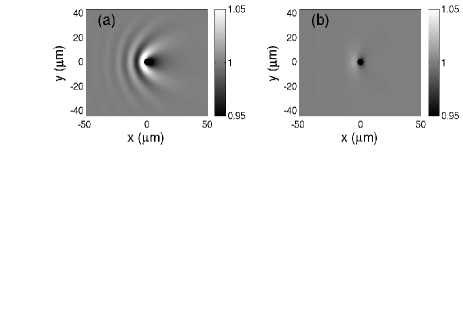
Figure 3: Real space resonant Rayleigh scattering emission pattern for a localized defect at $x=y=0$ acting on the cavity photon. The defect potential has a lateral size of $0.8\,\mu\textrm{m}$ and a depth of $1\,\textrm{meV}$. In panel (a), linear regime as in Fig.2(a) and (b). In panel (b), superfluid regime as in Fig.2(e) and (f). In each panel, the emitted intensity normalized to the transmitted intensity.

In the linear regime, the ${\bf k}$-space emission pattern shown in Fig.2(b) contains a peak at the incident wavevector ${\bf k}_{p}$, plus the RRS ring HoudreRRSLin ; Langbein . In the real space pattern shown in Fig.3(a), as the polariton fluid is moving to the right, the defect induces a propagating perturbation with parabolic wavefronts oriented in the left direction.

In the presence of interactions, the RRS circle is transformed into a $\infty$-like shape with the low-k lobe more intense than the high-k one. If $\Delta_{p}<0$, the two lobes are separated by a gap (Fig.2j), while they touch at ${\bf k}_{p}$ if $\Delta_{p}=0$ (Fig.2d). In this resonant case, when $\delta\omega_{MF}$ is large enough for the sound velocity $c_{s}$ in the polaritonic fluid to be larger than the flow velocity $v_{p}$, the slope of the $+$ branch on the low-k side of the corner (Fig.2e) becomes positive and there is no intersection with the horizontal dotted line any longer. In this regime, RRS is no longer possible, and the polaritonic fluid behaves as a superfluid in the sense of the Landau criterion Superfluidity . Once normalized to the incident one, the RRS intensity is strongly quenched with respect to the previous cases and no RRS ring is any longer present. The weak emission still visible in Fig.2(f) is due to non-resonant processes, which are allowed by the finite broadening of the polariton modes. As no propagating mode is resonantly excited, the perturbation in real space remains localized around the defect, as shown in Fig.3(b). On the other hand, on the bottom of the bistability curve (where $\Delta_{p}>0$), the polariton gas is not superfluid. The RRS intensity is even enhanced with respect to the linear regime because of the reduced linewidth of the Bogoliubov modes in the regions where the $\pm$ branches stick together, as shown in Fig.2(g-h).

To summarize, the polariton fluid has a superfluid behaviour with respect to static impurities if the equation $\omega_{LP}^{\pm}({\bf k})=\omega_{p}$ has no solutions with ${\bf k}\neq{\bf k}_{p}$. If the corresponding linear regime equation $\omega_{LP}({\bf k})=\omega_{p}$ has a set of solutions corresponding to the elastic RRS ring, the effect of superfluidity is dramatic as the RRS ring is suppressed. Within the parabolic approximation in Eq. (8), a simple sufficient condition for superfluidity is found: $\Delta_{p}\leq 0$ and $(m_{LP}v_{p}^{2}-\hbar\delta\omega_{MF})<\hbar|\Delta_{p}|$.

In conclusion, we have shown the strict connection between the dispersion of the elementary excitations in a quantum fluid of microcavity polaritons and the intensity and shape of the resonant Rayleigh scattering on defects. In particular, we have pointed out some experimentally accessible consequences of polaritonic superfluidity for realistic microcavity parameters. More in general, thanks to the coupling to externally propagating light, microcavity polaritonic systems appear to be promising candidates for the study of novel effects in low-dimensional quantum fluids.

We acknowledge G. C. La Rocca with whom the original idea of the work was conceived. We are grateful to Y. Castin and J. Dalibard for continuous discussions. LKB-ENS and LPA-ENS are two ”Unités de Recherche de l’Ecole Normale Supérieure et de l’Université Pierre et Marie Curie, associées au CNRS”.

References

- (1) D. Pines and P. Nozieres, The theory of quantum liquids Vols.1 and 2 (Addison-Wesley, Redwood City, 1966).
- (2) L. Pitaevskii and S. Stringari, Bose-Einstein condensation (Oxford University Press, 2003).
- (3) A. J. Leggett, Rev. Mod. Phys. 71, S318-S323 (1999).
- (4) C. Weisbuch et al., Phys. Rev. Lett. 69, 3314 (1992).
- (5) P. G. Savvidis et al., Phys. Rev. Lett. 84, 1547 (2000).
- (6) M. Saba et al., Nature (London) 414, 731 (2001).
- (7) C. Ciuti et al., Phys. Rev. B 62, R4825 (2000).
- (8) J. J. Baumberg et al., Phys. Rev. B 62, R16247 (2000).
- (9) G. Messin et al., Phys. Rev. Lett. 87, 127403 (2001).
- (10) For a recent review, see Semicond. Sci. Technol. 18, Special Issue on Microcavities, Guest Editors J. Baumberg and L. Viña, Publisher Sarah Quin (Bristol, UK, 2003).
- (11) H. Stolz et al., Phys. Rev. B 47, 9669 (1993).
- (12) R. Houdré et al., Phys. Rev. B 61, 13333R (2000).
- (13) R. Houdré et al., Phys. Rev. Lett. 85, 2793 (2000).
- (14) W. Langbein and J. M. Hvam, Phys. Rev. Lett. 88, 047401 (2002), and references therein.
- (15) For a review, see C. Ciuti, P. Schwendimann, and A. Quattropani, Semicond. Sci. Technol. 18, S279-S293 (2003) and references therein.
- (16) W. Langbein, proceedings of ICPS 26 (Edinburgh, UK, 2002).
- (17) S. Savasta, O. Di Stefano, and R. Girlanda, Phys. Rev. Lett. 90, 096403 (2003).
- (18) A. Baas et al., Phys. Rev. A 69, 023809 (2004).
- (19) N. A. Gippius et al., preprint cond-mat/0312214.
- (20) R. W. Boyd, Nonlinear Optics (Academic Press, London, 1992).
- (21) C. Ciuti, P. Schwendimann, A. Quattropani, Phys. Rev. B 63, 041303(R) (2001); D. M. Whittaker, Phys. Rev. B 63, 193305 (2001).
- (22) B. Wu and Q. Niu, Phys. Rev. A 64, 061603(R) (2001).