Implementation of Spin Hamiltonians in Optical Lattices

Abstract

We propose an optical lattice setup to investigate spin chains and ladders. Electric and magnetic fields allow us to vary at will the coupling constants, producing a variety of quantum phases including the Haldane phase, critical phases, quantum dimers etc. Numerical simulations are presented showing how ground states can be prepared adiabatically. We also propose ways to measure a number of observables, like energy gap, staggered magnetization, end-chain spins effects, spin correlations and the string order parameter.

In Condensed Matter Physics, there are strongly correlated systems of spins and electrons whose study is extremely difficult both analytically and numerically. These systems are of great practical interest since they may be relevant in some important instances like high-Tc superconductivity, to quote just one open problem of great relevance. These open problems have triggered a great number of models formulated by means of quantum many-body Hamiltonians like Heisenberg, t-J, Hubbard etc. Their quantum phase diagrams remain unknown for generic values of coupling constants, electron concentration (doping) and temperature, although a great knowledge can be obtained in particular integrable models in one dimension.

Two very important examples of these systems are quantum spin chains and ladders. Since the seminal work of Haldane Haldane quantum spin chains have been extensively studied as one of the simplest but most emblematic quantum many-body systems. According to Haldane, the one-dimensional integer-spin Heisenberg antiferromagnets have a unique disordered ground state with unbroken rotational symmetry and with a finite excitation gap in the spectrum, while half-integer antiferromagnets are gapless and critical. This quantum many-body phenomena is different from the usual source of gaps in magnets, namely, single-ion anisotropy, which does not involve quantum correlation effects. Several theoretical developments Haldane ; AKLT have helped to clarify the situation and there is now strong numerical evidence in support of Haldane’s claim.

Here we shall address the issue of implementing spin chains and ladders in an optical lattice. For concreteness, we focus on spin chains first. For integer spin, $s=1$, there is a quantum Hamiltonian that contains all the relevant information pertaining the Haldane phase and exhibiting a rich phase structure. This is the so–called Quadratic-Biquadratic Hamiltonian (QBH) given by

$$H_{\rm QB}=\alpha\sum_{i=1}^{N-1}\left[\vec{S}_{i}\cdot\vec{S}_{i+1}-\beta(\vec{S}_{i}\cdot\vec{S}_{i+1})^{2}\right]+\sum_{i=1}^{N}\vec{B}_{i}\vec{S}_{i}.$$ (1)

Here, $\vec{S}_{i}$ are spins $s=1$ at lattice site $i$, $\beta$ is a relative coupling constant that parametrizes a family of local Hamiltonians, and the sign of $\alpha$ determines the ferro or antiferromagnetic regimes. The properties of the ground state without magnetic field, $\vec{B}=0$, are entirely determined by an angle, $\theta$, such that $\alpha=|a|\cos(\theta)$ and $\alpha\beta=-|a|\sin(\theta)$ [See Fig. 1(a)]. For $\theta\in[-\frac{\pi}{4},\frac{\pi}{4}]$, the ground state belongs to the Haldane phase, with $\theta=0$ being the Heisenberg point and $\theta=\arctan(\frac{1}{3})$ the AKLT point AKLT , which is of particular importance because it can be described with an exact valence–bond wavefunction. There are two critical points on which the standard correlation length $\xi_{\rm C}$ diverges: $\theta=\frac{\pi}{4}$ is the Uimin-Lai-Sutherland (ULS) critical point ULS , where a phase transition occurs into a gapless phase for $\theta\in[\frac{\pi}{4},\frac{\pi}{2}]$; and $\theta=-\frac{\pi}{4}$ corresponds to the Takhtajan-Babujian (TB) critical point TB displaying a second order phase transition into a dimerized phase for $\theta\in[\frac{-3\pi}{4},-\frac{\pi}{4}]$, thus gapped. It has been conjectured that a quantum nondimerized nematic phase also exists chubukov in the ferromagnetic region.

Likewise, ladders of spin $s=\frac{1}{2}$ ladders exhibit a rich quantum phase structure depending on their number of legs and couplings: for even legs, ladders are gapped and can be in a Haldane phase similar to the integer spin chains, whereas for odd legs they are gapless. Even-legged ladders can also be in quantum dimer phases located on the rungs, provided the vertical couplings are strong enough. Theoretically, spin ladders are regarded as a route to approach the more complicate physics of two-dimensional quantum spin systems, as we increase the number of legs. For instance, a two-leg ladder is gapped and upon hole doping can serve as a toy model for studying superconducting correlations.

Experimental attempts to implement the QB Hamiltonian in real materials date back to the sixties. The first experimental evidence of a biquadratic term was found in Mn-doped MgO sixties and for $S=5/2$ $\rm Mn^{++}$ ions in antiferromagnetic chains of MnO sixties . The measured coupling constant was $\beta=-0.05$, too small and with a fixed sign. Thus, only the pure Heisenberg AF model and its immediate surroundings with a very small $\beta$ are of feasible practical implementation, and the AKLT point is rather far to be accessible. Experimentally, ladders can be realized by selective stoichiometric composition of cuprate planes in superconductors GRS . However, residual non-vanishing inter-ladder couplings on the planes introduce disturbances which are difficult to control.

Finding an experimental setup for checking the validity and observing the several phases of the QB Hamiltonian and of spin ladders is considered a very important challenge in the field. In this paper we propose to solve this problem using cold atoms confined in an optical lattice Bloch . As shown before, a Mott phase bh of cold atoms in a lattice can be described using ferromagnetic spin $s=\frac{1}{2}$ Duan ; njp or $s=1$ Yip03 ; Lukin Hamiltonians. Here we describe how to access a wider family of models, including Haldane phases of antiferromagnetic $s=1$ chains and $s=\frac{1}{2}$ ladders. We also design a technique to prepare adiabatically the atoms in the ground state, an important task since these spins cannot be cooled. Finally we study how to detect the different spin phases, and to directly observe correlation and excitation properties. This is in sharp contrast with standard experiments in condensed matter where one neither has a controllable implementation of the QB Hamiltonian (1) nor a direct way to perform measurements that so far have been regarded as mere theoretical tools.

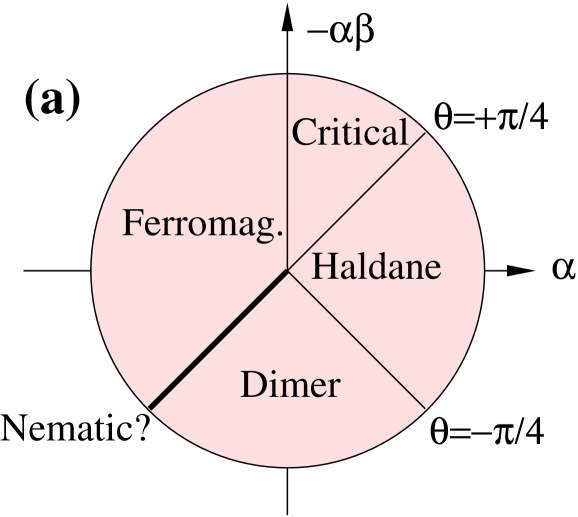
Figure 1: (a) Different phases of the ground state of Hamiltonian (1), according to the “angle” $\theta$ defined in the text. (b) Type of Hamiltonian (3) as a function of the gradient of the electric field, $\Delta$, for $U_{0}=0.75U_{2}$. The solid line is obtained naturally, the dashed line is for the dual model obtained when working on the upper part of the spectrum, and the dotted line marks the location of the possible nematic phase.

Let us first consider how to engineer Hamiltonian (1) using spin $s=1$ bosons in an array of one-dimensional optical lattices. For a strong confinement and low densities, the effective Hamiltonian is the Bose-Hubbard model bh

$$H = -J\sum_{\langle{j,l}\rangle,\alpha}(a^{\dagger}_{j\alpha}a_{l\alpha}+a^{\dagger}_{l\alpha}a_{j\alpha})+\sum_{j,\alpha}(E_{j}+B_{j\alpha})a^{\dagger}_{j\alpha}a_{j\alpha}$$ (2)

$$+ \sum_{S=0,2}\frac{U_{S}}{2}\sum_{j,\alpha,\beta,\gamma,\delta}(\Psi^{(S)}_{\sigma,\gamma\delta}a_{j\gamma}a_{j\delta})^{\dagger}(\Psi^{(S)}_{\sigma,\alpha\beta}a_{j\alpha}a_{j\beta}).$$

First of all, while the indices $j$ and $l$ run over the lattice sites, the Greek letters label the projection along the Z axis of either the spin of an atom ($\alpha,\beta,\gamma,\delta=-1,0,+1$), or of a pair of them ($\sigma=-2,-1,0,1,2$). Then the first term in the Hamiltonian is the single-particle hopping term and $J$ is the tunneling amplitude to a neighboring site. The second term models the interaction between bosons in a single site: two bosons can only interact if their total spin is either $0$ or $2$, because the state $S=1$ is antisymmetric. Furthermore, the interaction may be different for each value of the total spin. Both statements are summarized in the presence of spin-dependent interaction constants, $U_{S}$, and in the tensors $\Psi^{(S)}_{\sigma,\gamma\delta}=\langle{S,\sigma|s,\gamma;s,\beta}\rangle$, which are the Clebsch-Gordan coefficients between the states $|s=1,\gamma\rangle\otimes|s=1,\beta\rangle$ and $|S=0,2;\sigma\rangle$. Finally, we have included effective electric and magnetic fields, $E_{j}$ and $B_{j\alpha}$, that can be engineered using Stark shifts and spatially dependent magnetic fields, as in current experiments Bloch .

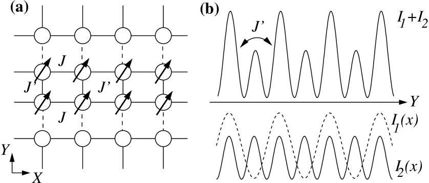
Figure 2: (a) A ladder is the combination of two spin chains that interact with each other. Interactions along a chain and between legs can be different. (b) We can build a ladder combining a 3D lattice, $I_{2}(x)$, with an additional 1D optical lattice, $I_{1}(x)$, that has twice the period of the first one. This induces a tunable hopping $J^{\prime}$, different from the longitudinal one, $J$, and suppresses hopping between neighboring ladders.

We will assume that the lattice has been loaded with one atom per site filtering , and that the tunneling has been strongly suppressed, $J\ll U_{S}$. With a perturbative calculation around states with unit occupation njp ; Yip03 ; Lukin we obtain the QB Hamiltonian (1) with constants

$$\alpha=\tfrac{1}{2}C_{2},\;\alpha\beta=-\tfrac{1}{6}(2C_{0}+C_{2}),\;C_{S}=\frac{J^{2}U_{S}}{\Delta^{2}-U_{S}^{2}}$$ (3)

This result is valid only if the gradient of the magnetic field is small, $|B_{j+1}-B_{j}|\ll|U_{S}|$, and the gradient of the electric field is constant, $\Delta=E_{j+1}-E_{j}$, and not resonant with the interaction, $|nU_{S}\pm\Delta|\gg J,\;\forall n\in\mathbb{Z}$.

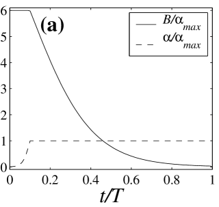
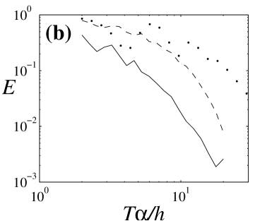
Figure 3: (a) Procedure for the adiabatic construction of the ground state of the $s=1$ antiferromagnet with open boundary conditions. (b) Infidelity of the final state for the AKLT (dashed), Heisenberg (solid) and $s=\frac{1}{2}$ spin ladder (dots), as a function of the duration of the process, for a setup with 9 spins (chains) or rungs (ladders).

In the absence of electric or magnetic fields the model reduces to that of Yip03 and Lukin , and we are restricted to a fixed value of $\theta$, typically in the ferromagnetic sector. However, with our tools it is possible to explore many other phases and achieve almost all values of $\theta$ [Fig. 3]. The idea is to change the gradient of the electric field and use a duality $H_{AF}=-H_{F}$ between ferro and antiferromagnetic models: The highest energy state of a ferromagnetic model ($\alpha<0$) is the same and exhibits the same dynamics as the ground state of the dual model ($-\alpha,-\beta$), since $\left(i\partial_{t}-H_{F}\right)\psi(t)=0\Leftrightarrow\left(i\partial_{t}-H_{AF}\right)\psi^{\star}(t)=0$. This equivalence is possible in current experiments, because dissipation is negligible and decoherence affects equally both ends of the spectrum.

A similar procedure is used for implementing ladders ladders of spin $s=\frac{1}{2}$. A ladder is nothing but the combination of two spin chains (legs) that interact with each other. To build them we need to set up a 3D lattice that confines the atoms on planar square lattices (hopping has been suppressed along the $Z$ direction), and superimpose along the $Y$ direction a second 1D lattice with twice the period [Fig. 2(b)]. Adjusting the intensities of different lattices we can modify the tunneling along the leg of a ladder and between neighboring legs, and completely suppress tunneling between ladders. With the help of electric and magnetic fields njp , and the duality between ferro and antiferromagnetic models, we achieve once more a full tunability of the Hamiltonian.

Let us now study how to prepare ground states adiabatically. We will focus on the Haldane phase of the $s=1$ lattice and on the antiferromagnetic $s=\frac{1}{2}$ ladders. Since in both cases we seek an antiferromagnetic state, we can begin with a configuration of antiparallel spins, an effective staggered magnetic field, $B_{j}=(-1)^{j}|B(t)|$, and no hopping. We then progressively decrease the magnetic field and increase the interaction, $\alpha$ [See Fig. 3(a)]. This procedure constrains us to a subspace of fixed magnetization, $\langle{\sum_{j}S^{z}_{j}}\rangle\simeq 0$, and also ensures that the minimum energy gap between the ground state and the first excitations remains independent of the number of spins. Thus, the speed of the adiabatic process can be the same for all lattice sizes, an important point in a setup with defects.

We have studied numerically the fidelity of the adiabatic process for the AKLT point, for $\beta=0$, and for a $s=\frac{1}{2}$ ladder, using different speeds and sizes. The fidelity is the projection of the final state onto the (degenerate) ground states (in the case of $s=1$, it is one singlet and three triplet states). The results are shown in Fig. 3(b). Already for a duration of $10\times h/\alpha_{max}$ the Haldane phase is built with $99\%$ fidelity. Assuming current optical lattices, with $U/h\simeq 3$KHz and $J=0.3U$, this implies a time of roughly $37$ ms. Improvements on these values are expected with the implementation of optically induced Feschbach resonances feschbach .

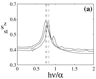
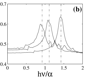
Figure 4: Maximum staggered magnetization per spin acquired by the ground state of the (a) AKLT and (b) Heisenberg models, under an oscillating magnetic field, $B_{j}=(-1)^{j}0.025\alpha\cos(2\pi\nu t)$, for $5$, $7$ and $9$ spins (right to left). Vertical lines mark the finite excitation gap for the given size.

Regarding the staggered magnetic field, for ⁸⁷Rb in the $F=1$ hyperfine state it can be produced using a weaker optical lattice, aligned with the atomic chains and made of a pair of counterpropagating laser beams in a lin $\perp$ lin configuration. If the lasers are far off-resonance from the transition ${}^{2}\mathrm{S}\to{}^{2}\mathrm{P}$, we will obtain a state-dependent potential $V_{\perp}(x)\propto 2+(\sin(kx)^{2}-\cos(kx)^{2})S_{z}$, where the $\sin(kx)$ and $\cos(kx)$ come from the Stark shifts induced by the $\sigma_{+}$ and $\sigma_{-}$ polarizations on the atomic states. Choosing the orientation of the counterpropagating beams so that $V_{\perp}(x)$ has twice the periodicity of the confining lattice we get our staggered magnetic field. A similar setup can be designed for $s=\frac{1}{2}$ particles.

Once we have constructed the ground state, we would like to study its properties. We will describe a number of possible experiments, sorted by increasing difficulty. For illustrative purposes, we consider the Haldane phase of a $s=1$ spin chain, but we want to emphasize that the same techniques can be applied to other phases, spin models and even ladders. Preliminary evidences of the Haldane phase can be obtained by studying global properties, such as the staggered magnetization, $\vec{S}_{st}=\sum_{j}(-1)^{j}\vec{S}_{j}$, which is zero in the dimer phase and nonzero in the Haldane phase. To measure $S_{st}^{x,y}$, we apply a $\pi/2$ rotation around the $Z$ axis using the staggered magnetic field, and then measure $\langle\sum_{i}S_{i}^{x,y}\rangle$. The remaining component $S_{st}^{z}$ can be obtained by rotating all spins an angle $\pi/2$ around the $X$ or $Y$ axes, and then measuring $S_{st}^{y}$ or $S_{st}^{x}$.

We can also study the energy gap between the ground state and its excitations, using an oscillating magnetic field, $B_{j}(t)=(-1)^{j}B\sin(\omega t)$. From linear response theory we know that for small intensities, $|B|\ll\alpha$, there is a strong resonance at the gap, $\hbar\omega=E_{gap}$, which manifests itself on the growth of the staggered magnetization, $S^{z}_{st}$. This result has been confirmed by numerical simulations of small lattices, as shown in Fig. 4.

Another interesting feature of the Haldane phase are fractionalization effects. To understand this, one should visualize each atom with spin $s=1$ as being composed of two $s=\frac{1}{2}$ bosons in a symmetric state. The ground state of Eq. (1) can then be built —either approximately, if $\beta\neq 1/3$, or exactly, for the AKLT—, by antisymmetrizing pairs of virtual spins from neighboring sites AKLT . This leaves us with two free effective $s=\frac{1}{2}$ spins at the ends of a chain, which manifest themselves physically. First, the four almost degenerate ground states are determined by the values of the free virtual spins, which we will denote as $\left|i_{1},i_{2N}\right\rangle$. Thus, if the state of the system is $\left|\psi\right\rangle=\sum_{ij}c_{ij}\left|i,j\right\rangle$, the probability of measuring the left- and rightmost real spins in states $I,J=\pm 1$ is approximately $4|c_{I/2,J/2}|^{2}/9$. And second, the virtual spins almost do not interact and can be manipulated independently with weak magnetic fields that have different values on the borders of a chain. For instance, if we prepare the ground state using our method, apply a global rotation of angle $\theta=\frac{\pi}{2}$ around the $Y$ axis, and then switch on the staggered magnetic field, we will measure periodic oscillations in the value of $S^{x}_{st}$, because the virtual spins on even and odd sites rotate with opposite senses.

We also have developed a procedure to measure spin correlation functions in optical lattices, an essential tool for experiments with spin lattices. Our proposal only assumes that we can trap atoms in separate lattices and empty lattice sites with double occupation . First of all, we notice that a spin correlation may be written as a density correlation, $\langle S^{z}_{j}S^{z}_{k}\rangle=\langle n^{+1}_{j}n^{+1}_{k}+n^{-1}_{j}n^{-1}_{k}-n^{+1}_{j}n^{-1}_{k}-n^{-1}_{j}n^{+1}_{k}\rangle$, where $n^{\alpha}_{k}$ is the number of atoms in hyperfine state $\alpha$ on the $k$-th site. A correlation such as $\sum_{j}\langle n^{1}_{j}n^{1}_{j+\Delta}\rangle$ can be measured by moving the atoms of species $+1$ just $\Delta$ sites qc ; bloch-qc , emptying all doubly occupated sites and counting the number of atoms left in state $+1$, on the sites $j$ and $k$. If we rather count the atoms in state $0$, then we will obtain $\langle n^{-1}_{j}n^{+1}_{k}\rangle$. With this method, and some global rotation of the spins, it is possible to obtain all correlators, $\langle\vec{S}_{j}\vec{S}_{j+\Delta}\rangle$. If we cannot address individual atoms, using the same procedure and measuring total populations, $\sum_{k}n^{\alpha}_{k}$, we will obtain averaged values, $\sum_{k}\langle\vec{S}_{j}\vec{S}_{j+\Delta}\rangle$. Both quantities are interesting to discriminate between the different spin phases.

On a much higher level of difficulty, but with pretty much the same tools as for measuring correlations we can obtain the string order parameters string-order . One can show that it is equivalent to a correlation function measured on a transformed state,

$${\cal S}_{km} := \left\langle S^{z}_{k}e^{i\pi\sum_{j=k+1}^{m-1}S^{z}_{j}}S^{z}_{m}\right\rangle_{\psi}=\left\langle S^{z}_{k}S^{z}_{m}\right\rangle_{U_{m-k}\psi},$$ (4a)

$$U_{\Delta} = \exp\left[i\pi\sum_{k=1}^{N}\sum_{j=k+1}^{k+\Delta}\left(1-{S^{z}_{k}}^{2}\right)S^{x}_{j}\right]$$ (4b)

The unitary operation $U_{\Delta}$ can be performed as follows. First we perform half a swap between the $+1$ and $-1$ states, $U_{1}=\exp\left[i\pi/2\sum_{k}(\left|+1\right\rangle\left\langle-1\right|_{k}+\left|-1\right\rangle\left\langle+1\right|_{k})\right]$, with a $\pi/2$ Raman pulse that connects these states. Next we split the three species into three optical lattices. The atoms in state $0$ will move $\Delta-1$ sites to the right, and on each movement a controlled collision with atoms in state $+1$ will take place. Adjusting the duration of this collision so that it produces a phase of $\pi$, we obtain the transformation $U_{2}=\exp\left[i\sum_{k}\sum_{j=1}^{\Delta-1}(\left|0\right\rangle\left\langle 0\right|_{k}\left|+1\right\rangle\left\langle+1\right|_{k+j})\right]$. We restore all atoms back to their positions, and repeat the operation $U_{1}$, concluding the total transformation $U_{\Delta}=U_{1}U_{2}U_{1}$. Finally, we perform all required steps to measure either $\langle S^{z}_{k}S^{z}_{k+\Delta}\rangle$ or $\sum_{k}\langle S^{z}_{k}S^{z}_{k+\Delta}\rangle$.

Typical experiments have defects and thus host chains with different number of spins. However, except for the string-order parameter, the measurements that we propose are extremely robust, and in general they produce a signal that is a nonzero average of the possible outcomes for chains of different lengths.

Summing up, in this work we have shown how to implement spin $s=1$ chains and $s=\frac{1}{2}$ ladders with cold atoms in an optical lattice. Such experiments will allow us to construct never observed phases and probably dilucidate the existence of the nematic phase. Finally, we have developed a very general set of tools to characterize these spin phases, which are themselves of interest for future experiments with optical lattices.

This work has been supported by the EU projects TOPQUIP and CONQUEST, Kompetenznetzwerk Quanteninformationsverarbeitung der Bayerischen Staatsregierung, SFB631, and DGES under Contract BFM2000-1320-C02-01.

References

- (1) F.D.M. Haldane, Phys. Lett. 93A, 464 (1983); Phys. Rev. Lett. 50, 1153 (1983).
- (2) I. Affleck, T. Kennedy, E.H. Lieb and H. Tasaki, Commun. Math. Phys. 115, 477 (1988); Phys. Rev. Lett. 59, 799 (1987).
- (3) G.V. Uimin, JETP Lett. 12, 225 (1970); C.K. Lai, J. Math. Phys. 15 1675 (1974); B. Sutherland, Phys. Rev. B 12, 3795 (1975).
- (4) L.A. Takhtajan, Phys. Lett. A 87, 479 (1982); H.M. Babujian, Phys. Lett. A 90, 479.
- (5) A. V. Chubukov, Phys. Rev. B 43, 3337 (1991).
- (6) E. Dagotto and T.M. Rice, Science 271, 618 (1996).
- (7) S. Gopalan, T.M. Rice, and M. Sigrist, Phys. Rev. B 49, 8901 (1994).
- (8) E.A. Harris, J. Owen; Phys. Rev. Lett. 11, 10 (1963); D. S. Rodbell, I. S. Jacobs, and J. Owen,E. A. Harris, ibid. 11, 9 (1963).
- (9) M. Greiner, O. Mandel, T. Esslinger, Th. W. Hänsch, and I. Bloch, Nature 415, 39 (2002); M. Greiner, O. Mandel, Th. W. Hänsch, and I. Bloch, Nature 419, 51 (2002).
- (10) L.-M. Duan, E. Demler, and M. D. Lukin Phys. Rev. Lett. 91, 090402 (2003).
- (11) J. J. García-Ripoll, and J. I. Cirac, New Journal of Physics (2003).
- (12) S. K. Yip, Phys. Rev. Lett. 90, 250402 (2003).
- (13) A. Imambekov, M. Lukin, and E. Demler, arXiv:cond-mat/0306204; A. Imambekov, M. Lukin, and E. Demler, arXiv:cond-mat/0401526.
- (14) D. Jaksch, C. Bruder, J. I. Cirac, C. W. Gardiner, and P. Zoller Phys. Rev. Lett. 81, 3108-3111 (1998)
- (15) P. Rabl, A. J. Daley, P. O. Fedichev, J. I. Cirac, and P. Zoller, Phys. Rev. Lett. 91, 110403 (2003).
- (16) P. O. Fedichev, Yu. Kagan, G. V. Shlyapnikov, and J. T. M. Walraven, Phys. Rev. Lett. 77, 2913-2916 (1996); I. Bloch, private communication.
- (17) D. Jaksch, H.-J. Briegel, J. I. Cirac, C. W. Gardiner, and P. Zoller Phys. Rev. Lett. 82, 1975 (1999); D. Jaksch, Ph. D. Thesis.
- (18) O. Mandel, M. Greiner, A. Widera, T. Rom, T. W. Hänsch, and I. Bloch Phys. Rev. Lett. 91, 010407 (2003).
- (19) M. den Nijs and K. Rommelse, Phys. Rev. B 40, 4709 (1989); H. Tasaki, Phys. Rev. Lett. 66, 798 (1991); T. Kennedy and H. Tasaki, Phys. Rev. B 45, 304 (1992); M. Oshikawa, J. Phys.: Condens. Matter 4, 7469 (1992).