Self-interaction corrected relativistic theory of magnetic scattering of x rays: Application to praseodymium

Abstract

A first-principles theory of resonant magnetic scattering of x rays is presented. The scattering amplitudes are calculated using a standard time-dependent perturbation theory to second order in the electron-photon interaction vertex. In order to calculate the cross section reliably an accurate description of the electronic states in the material under investigation is required and this is provided by the density functional theory (DFT) employing the Local Spin Density Approximation combined with the self-interaction corrections (SIC-LSD). The magnetic x-ray resonant scattering (MXRS) theory has been implemented in the framework of the relativistic spin-polarized LMTO-ASA band structure calculation method. The theory is illustrated with an application to ferromagnetic praseodymium. It is shown that the theory quantitatively reproduces the dependence on the spin and orbital magnetic moments originally predicted qualitatively (Blume, J. Appl. Phys, 57, 3615 (1985)) and yields results that can be compared directly with experiment.

I Introduction

Magnetic X-Ray Scattering (MXRS) is a well developed technique for probing the magnetic and electronic structures of materials. The foundations of the theory of MXRS were laid down by Blume. Blum85 Later on Blume and Gibbs Blum88 developed the theory further to show that the orbital and spin contributions to the magnetic moment can be measured separately using MXRS with a judicious choice of experimental geometry and polarization of the x rays. Hannon et al. Hann88 presented a nonrelativistic theory of x-ray resonance exchange scattering and wrote down explicit expressions for the electric dipole ($E1$) and quadrupole ($E2$) contributions. This work is based on an atomic model of magnetism and has been applied successfully to a variety of materials including UAs and Gd by Fasolino et al.. Faso93 Rennert Renn93 produced a semi-relativistic theory of MXRS written in terms of Green’s functions, but no such calculations have been performed. More recently, theory based on an atomic model of the electronic structure of materials has been written down by Lovesey Love and co-workers and applied successfully to a variety of materials. Takahashi et al. have reported a theory which includes the band structure in the calculation of anomalous x-ray scattering. Taka A first-principles theory of MXRS based on a time-dependent second order perturbation theory and density functional theory hohen65 ; Kohn+Vash was produced by Arola et al. Eero97 ; Eero01 and applied successfully to several transition metal materials. Eero98 This theory is restricted in its range of application because of the limitations imposed by the local density approximation to DFT which means that the theory can only be applied to simple and transition metal materials. This is particularly unfortunate because it is in the rare earth and actinide materials that the most exotic magnetism in the periodic table occurs.

In recent years advances in electronic structure calculations beyond the local density approximation have broadened the range of materials for which numerically accurate electronic structure calculations can be performed. In particular the LDA+U method anis93 and the self-interaction corrected local spin density approximation to density functional theory Fuji95 ; Dzid93 ; Bris97 ; Svan90 have met with considerable success in describing materials with localized electrons. The latter method reduces the degeneracy of the $f$ states at the Fermi level and hence also circumvents all the convergence problems associated with the LSD approximation to DFT in electronic structure calculations for rare earth materials. Notably, the SIC-LSD has provided a very good description of the rare earth metal and rare earth chalcogenide crystal structures. nature A relativistic version of the SIC formalism has been derived Beid97 that has been shown to yield an excellent description of the electronic structure of rare earth materials in the few cases to which it has been applied. This method is reviewed by Temmerman et al.. Bris97

The fact that electromagnetic radiation can be scattered from the magnetic moments of spin-1/2 particles was first shown by Low, and by Gell-Mann and Goldberger half a century ago. Low54 Later on it was Platzman and Tzoar Plat70 who first proposed the use of x-ray scattering techniques to study the magnetization density of solids. At that time progress in studying magnetic structures using x rays was severely hampered because the cross section for magnetic scattering is smaller than the cross section for charge scattering Blum85 by a factor of $(\hbar\omega/mc^{2})^{2}$. It was Gibbs et al. Gibb88 who first observed a large resonant enhancement of the cross section when the energy of the x ray is tuned through an absorption edge. Since that time technological advances have produced high resolution, high intensity synchrotron radiation sources that have transformed magnetic x-ray resonant scattering into a practical tool for investigating magnetic and electronic structures of materials. Nowadays the world’s leading synchrotron facilities have beamlines dedicated to this technique Coop01 and applications of resonant x-ray scattering are burgeoning. Reviews of the experimental state-of-the-art MXRS techniques have been written by Stirling Stir99 and Cooper. Coop99

Other approaches to interpreting MXRS spectra exist, particularly the successful methods based on group theory and angular momentum algebra that result in sum rules as described by Borgatti Laan04 and by Carra Paolo and Luo. Luo The present work should not be regarded as a rival theory to these, but rather as an attempt to extend the range of density functional methods to describe magnetic scattering of x rays in the same way as is done for photoemission and other spectroscopies. Durh84 As a DFT-based theory our work is, of course, based on very different approximations to this earlier work, making direct comparison between the two theories problematic.

We have recently implemented a first-principles theory of MXRS that is based on a standard time-dependent perturbation theory where the scattering amplitudes are calculated to second order in the electron-photon interaction vertex. To describe MXRS from a given material it is necessary to have an accurate description of the electronic structure of the material in question. This is provided by using the SIC within the LSD approximation to the density functional theory which is implemented using the relativistic spin-polarized LMTO-ASA band structure calculation method. tblmto The theory of MXRS is equivalent to that of Arola et al., Eero97 but has been rewritten in a form that is appropriate for implementation in connection with the LMTO-ASA method where there is substantial experience of SIC methods. The major step forward reported in this paper is the integration of the SIC into the MXRS theory which enables us to describe rare earth and actinide materials on an equal footing with transition and simple materials.

In this paper, we give a detailed description of the MXRS theory and illustrate it in a calculation for praseodymium. The results are analysed and discussed. Finally we show that the present work is consistent with the earlier theory and demonstrate how the MXRS cross section reflects the properties of these materials.

II Theory

II.1 The relativistic SIC-LSD formalism

The SIC-LSD approximation ZP ; Comment is an ab-initio electronic structure scheme, that is capable of describing localization phenomena in solids. Bris97 ; Svan90 ; Dzid93 In this scheme the spurious self-interaction of each occupied electron state is subtracted from the conventional LSD approximation to the total energy functional, which leads to a greatly improved description of static Coulomb correlation effects over the LSD approximation. This has been demonstrated in studies of the Hubbard model, Rapid ; vogl-hub in applications to 3$d$ monoxides Dzid93 ; Svan90 and cuprates, PRL2 ; Dzid93 $f$-electron systems, nature ; walt3 ; leon orbital ordering, rik metal-insulator transitions temm4 and solid hydrogen. SSC

For many applications it is necessary to account for all relativistic effects including spin-orbit coupling in an electronic structure calculation. Relativistic effects become progressively more important as we proceed to heavier elements. They are also extremely important when we are considering properties dependent on orbital moments and their coupling to electron spins.

The relativistic total energy functional in the local spin density approximation is

$$E^{\rm LSD}[{\overline{n}}({\bf r})] = E_{\rm kin}[n({\bf r})]+U[n({\bf r})]+\int V^{\rm ext}({\bf r})n({\bf r})d^{3}r$$ (1a)

$$+ E^{\rm LSD}_{\rm xc}[{\overline{n}}({\bf r})]-\int{\bf B}^{\rm ext}({\bf r})\cdot{\bf m}({\bf r})d^{3}r,$$

where $${\overline{n}}({\bf r})=(n^{\uparrow}({\bf r}),n^{\downarrow}({\bf r}))(\equiv(n({\bf r}),m({\bf r})))$$ labels the spin up and spin down charge density.

$$E_{\rm kin}[n({\bf r})] = \sum_{\Lambda}<\psi_{\Lambda}|{\hat{T}}|\psi_{\Lambda}>,$$ (1b)

$$E^{\rm LSD}_{xc}[{\overline{n}}({\bf r})] = \int n({\bf r})\epsilon_{xc}[{\overline{n}}({\bf r})]d^{3}r.$$ (1c)

Here ${\hat{T}}$ is an operator describing the kinetic energy and rest mass of the electrons

$${\hat{T}}=\frac{c\hbar}{i}{\bm{\alpha}}\cdot\nabla+mc^{2}(\beta-I_{4}),$$ (2)

where ${\bm{\alpha}}$ and $\beta$ are the usual relativistic matrices Stra98 . $U[n({\bf r})]$ represents all two particle interactions including the Breit interaction. $V^{\rm ext}({\bf r})$ is the external potential, ${\bf B}^{\rm ext}({\bf r})$ is an external magnetic field. The density $n({\bf r})$ and the spin density ${\bf m}({\bf r})$ are given by

$$n({\bf r})=\sum_{\Lambda}\psi^{{\dagger}}_{\Lambda}({\bf r})\psi_{\Lambda}({\bf r}),$$ (3)

$${\bf m}({\bf r})=-\mu_{\bf B}\sum_{\Lambda}\psi^{{\dagger}}_{\Lambda}({\bf r})\beta{\bm{\sigma}}_{4}\psi_{\Lambda}({\bf r}),$$ (4)

where ${\bm{\sigma}}_{4}$ is the $4\times 4$ matrix spin operator and $\Lambda$ represents the quantum numbers. In Eqs. (II.1) and (II.1) below we have implied a representation in which spin is a good quantum number and the sums are over the occupied states. $\epsilon_{xc}[{\overline{n}}({\bf r})]$ is the exchange correlation energy of a gas of constant density and Eq. (1c) is the local spin density approximation.

If we minimise the functional (1a) with respect to changes in the density and spin density we obtain a Dirac-like equation:

$$(\frac{c\hbar}{i}{\bm{\alpha}}\cdot\nabla + mc^{2}(\beta-I_{4})+V^{\rm eff}({\bf r})$$ (5a)

$$+ \mu_{\rm B}\beta{\bm{\sigma}}_{4}\cdot{\bf B}^{\rm eff}({\bf r}))\psi_{\Lambda}({\bf r})=\epsilon_{\Lambda}\psi_{\Lambda}({\bf r}),$$

where

$$V^{\rm eff}({\bf r}) = V^{\rm ext}({\bf r})+\frac{e^{2}}{4\pi\epsilon_{0}}\int\frac{n({\bf r^{\prime}})}{|{\bf r}-{\bf r^{\prime}}|}d^{3}r^{\prime}$$ (5b)

$$+ \frac{\delta E^{\rm LSD}_{xc}[{\overline{n}}({\bf r})]}{\delta n({\bf r})},$$

$${\bf B}^{\rm eff}({\bf r}) = {\bf B}^{\rm ext}({\bf r})-\frac{\delta E^{\rm LSD}_{xc}[{\overline{n}}({\bf r})]}{\delta{\bf m}({\bf r})},$$ (5c)

where ${\overline{n}}({\bf r})\equiv(n^{\uparrow}({\bf r}),n^{\downarrow}({\bf r}))(\equiv(n({\bf r}),{\bf m}({\bf r})))$. The local spin density approximation discussed above provides a very successful description of a variety of properties of condensed matter, but suffers from a drawback because it contains self-interactions of the single particle charges. In an exact theory these spurious self-interactions would precisely cancel. In the LSD the cancellation is only approximate and in materials where there are well-localised electrons this can lead to significant errors. The SIC-LSD approach to this problem is to augment the LSD functional with an extra term that removes this deficiency. Beid97

$$E^{\rm SIC-LSD}=E^{\rm LSD}+E^{\rm SIC},$$ (6a)

where

$$E^{\rm SIC}[\{{\overline{n}}_{\gamma}({\bf r})\}]=-\sum_{\gamma}(U[n_{\gamma}({\bf r})]+E_{\rm xc}^{\rm LSD}[{\overline{n}}_{\gamma}({\bf r})],$$ (6b)

where $${\overline{n}}_{\gamma}({\bf r})\equiv(n_{\gamma}^{\uparrow}({\bf r}),n_{\gamma}^{\downarrow}({\bf r}))(\equiv(n_{\gamma}({\bf r}),{\bf m}_{\gamma}({\bf r})))$$ and

$$U[n_{\gamma}({\bf r})]=\frac{1}{2}\frac{e^{2}}{4\pi\epsilon_{0}}\int\int\frac{n_{\gamma}({\bf r})n_{\gamma}({\bf r}^{\prime})}{|{\bf r}-{\bf r}^{\prime}|}d^{3}r^{\prime}d^{3}r,$$ (6c)

$$E^{\rm LSD}_{\rm xc}[{\overline{n}}_{\gamma}({\bf r})]=\int n_{\gamma}({\bf r})\epsilon_{\rm xc}[{\overline{n}}_{\gamma}({\bf r})]d^{3}r,$$ (6d)

where $$\gamma$$ runs over all orbitals that are SI-corrected, and

$$n_{\gamma}({\bf r})\equiv\psi^{{\dagger}}_{\gamma}({\bf r})\psi_{\gamma}({\bf r}),$$ (6e)

$${\bf m}_{\gamma}({\bf r})\equiv-\mu_{\bf B}\psi^{{\dagger}}_{\gamma}({\bf r})\beta{\bm{\sigma}}_{4}\psi_{\gamma}({\bf r}),$$ (6f)

For the exchange-correlation term in the SIC energy we need to consider a fully spin-polarised electron. The corresponding single particle-like wave equation is obtained by taking the functional derivative of $E^{\rm SIC-LSD}$ with respect to $\psi^{*}_{\gamma}({\bf r})$ and we obtain

$$(\frac{c\hbar}{i}{\bm{\alpha}}\cdot\nabla + mc^{2}(\beta-I_{4})+V^{\rm eff}({\bf r})+\mu_{\rm B}\beta{\bm{\sigma}}\cdot{\bf B}^{\rm eff}({\bf r})$$ (7a)

$$+ V^{\rm SIC}_{\gamma}({\bf r}))\psi_{\gamma}({\bf r})=\sum_{\gamma^{\prime}}\lambda_{\gamma,\gamma^{\prime}}\psi_{\gamma^{\prime}}({\bf r}),$$

where the SIC potential is given by

$$V^{\rm SIC}_{\gamma}({\bf r})=-\left(\frac{e^{2}}{4\pi\epsilon_{0}}\int\frac{n_{\gamma}({\bf r^{\prime}})}{|{\bf r}-{\bf r}^{\prime}|}d{\bf r}^{\prime}\right.$$ (7b)

$$+ \left.\frac{\delta E^{\rm LSD}_{\rm xc}[{\overline{n}}_{\gamma}({\bf r})]}{\delta n_{\gamma}({\bf r})}-\mu_{\rm B}\beta{\bm{\sigma}}_{4}\cdot\frac{\delta E^{\rm LSD}_{\rm xc}[{\overline{n}}_{\gamma}({\bf r})]}{\delta{\bf m}_{\gamma}({\bf r})}\right).$$

The task of finding the single particle-like wavefunctions is now considerably more challenging than for the bare LSD because every state experiences a different potential. To maintain the orthogonality of the $\psi_{\gamma}({\bf r})$ it is necessary to calculate the Lagrange multiplier matrix, $\lambda_{\gamma\gamma^{\prime}}$.

As written in Eqs. (10-13), $E^{\rm SIC-LSD}$ appears to be a functional of the set of occupied orbitals rather than of the total spin density only, like $E^{\rm LSD}$. By a reformulation it may be shown ZP ; Comment that $E^{\rm SIC-LSD}$ can in fact be regarded as a functional of the total spin density only. The associated exchange-correlation energy functional $E_{\rm xc}^{\rm SIC}[{\overline{n}}({\bf r})]$ is, however, only implicitly defined, Comment for which reason the associated Kohn-Sham equations are rather impractical to exploit. For periodic solids the SIC-LSD approximation is a genuine extension of the LSD approximation in the sense that the self-interaction correction is only finite for localized states, which means that if all valence states considered are Bloch-like single-particle states $E^{\rm SIC-LSD}$ coincides with $E^{\rm LSD}$. Therefore, the LSD minimum is also a local minimum of $E^{\rm SIC-LSD}$. In some cases another set of single-particle states may be found, not necessarily in Bloch form but, of course, equivalent to Bloch states, to provide a local minimum for $E^{\rm SIC-LSD}$. For this to happen some states must exist which can benefit from the self-interaction term without losing too much band formation energy. This usually will be the case for rather well localized states like the 3$d$ states in transition metal oxides or the 4$f$ states in rare earth compounds. Thus, $E^{\rm SIC-LSD}$ is a spin density functional, which may be used to describe localized as well as delocalized electron states.

We have solved the SIC-LSD equations self-consistently for a periodic solid using the unified Hamiltonian approach described by Temmerman et al.. Temm3 The equations have been solved on a periodic lattice using the relativistic LMTO method in the tight-binding representation.

II.2 The relativistic spin-polarised LMTO method

In Section II C, $u_{\Lambda^{\prime}}({\bf r})$ will be a general notation for the unoccupied intermediate states in the second order time-dependent perturbation theory. In the case of a material with translational periodicity $u_{\Lambda^{\prime}}({\bf r})$ will be a Bloch state

$$u_{\Lambda^{\prime}}({\bf r})=\psi^{j{\bf k}}({\bf r}),$$ (8)

for which

$$\psi^{j{\bf k}}({\bf r}+{\bf R})=e^{i{\bf k}\cdot{\bf R}}\psi^{j{\bf k}}({\bf r}),$$ (9)

where ${\bf k}$ is the wavevector defined to be in the first Brillouin zone, $j$ is the band index, and ${\bf R}$ is any Bravais lattice vector. In the LMTO method the Bloch wave functions may be expanded in several ways. tblmto For the calculation of observables it is most convenient to make an expansion in terms of the single-site solutions of the radial Dirac equation and their energy derivatives. For the relativistic spin-polarised case this has been achieved by Ebert Ebert88 ; Ebert882 and it is this method that we employ. The Bloch state in this representation is written as

$$\psi^{j{\bf k}}({\bf r}) = \sum_{t=1}^{N_{\rm type}}\sum_{i=1}^{N_{t}}\sum_{\Lambda}\left[\right.A^{j{\bf k}}_{ti\Lambda}\phi_{\nu t\Lambda}({\bf r}-{\bm{\tau}}^{(t)}_{i})$$ (10a)

$$+ B^{j{\bf k}}_{ti\Lambda}{\stackrel{{\scriptstyle.}}{{\phi}}}_{\nu t\Lambda}({\bf r}-{\bm{\tau}}^{(t)}_{i})\left.\right].$$

Here

$$\phi_{\nu t\Lambda}({\bf r}^{(t)}_{i})=\sum_{\kappa^{\prime}}\left(\begin{matrix}g^{{(t)}m_{j}}_{\kappa^{\prime}\kappa}(\epsilon_{\nu},r^{(t)}_{i})\chi^{m_{j}}_{\kappa^{\prime}}({\hat{\bf r}}^{(t)}_{i})\cr if^{{(t)}m_{j}}_{\kappa^{\prime}\kappa}(\epsilon_{\nu},r^{(t)}_{i})\chi^{m_{j}}_{-\kappa^{\prime}}({\hat{\bf r}}^{(t)}_{i})\cr\end{matrix}\right),$$ (10b)

where the $g^{(t)m_{j}}_{\kappa^{\prime}\kappa}(E,r^{(t)}_{i})$ and $f^{(t)m_{j}}_{\kappa^{\prime}\kappa}(E,r^{(t)}_{i})$ are solutions of the radial Dirac equation for a spin-polarised system, and ${\bf r}^{(t)}_{i}\equiv{\bf r}-{\bm{\tau}}^{(t)}_{i}$. Details of the solution are given in by Strange et al., Stra84 and ${\stackrel{{\scriptstyle.}}{{\phi}}}_{\nu t\Lambda}({\bf r}^{(t)}_{i})$ is its energy derivative. These satisfy

$$\langle\phi_{\nu t\Lambda}|\phi_{\nu t\Lambda}\rangle=1\hskip 42.67912pt\langle\phi_{\nu t\Lambda}|{\stackrel{{\scriptstyle.}}{{\phi}}}_{\nu t\Lambda}\rangle=0,$$ (11)

where the subscript $\nu$ corresponds to the energy $\epsilon_{\nu}$ about which the muffin-tin orbitals of Eq. (10b) are expanded, and the normalization integrals have been done within the atomic sphere $S^{t}$. The single particle functions $\phi_{\nu t\Lambda}({\bf r})$ and ${\stackrel{{\scriptstyle.}}{{\phi}}}_{\nu t\Lambda}({\bf r})$ are evaluated at energy $\epsilon_{\nu}$. In this relativistic formulation $\Lambda\equiv(\kappa m_{j})$ labels the boundary condition for the independent single-site solution $\phi_{\nu t\Lambda}({\bf r}-{\bm{\tau}}^{(t)}_{i})$ of the Dirac equation about the basis atom at ${\bm{\tau}}^{(t)}_{i}$. $N_{\rm type}$ is the number of different types of atom in the unit cell. $N_{t}$ is the number of equivalent atoms of type $t$. The coefficients $A^{j{\bf k}}_{ti\Lambda}$ and $B^{j{\bf k}}_{ti\Lambda}$ are written in terms of the LMTO structure constants and potential parameters, and are completely determined by a self-consistent LMTO calculation of the electronic structure. tblmto Key observables are then given in terms of these quantities. In particular the spin moment is

$$m_{S}=\sum_{j}\int_{\epsilon^{j{\bf k}}<\epsilon_{\rm F}}m^{j{\bf k}}_{s}d^{3}k,$$ (12a)

where

$$m^{j{\bf k}}_{s} = \sum_{t,i}\sum_{\Lambda}\sum_{\Lambda^{\prime}}\left(A^{j{\bf k}*}_{ti\Lambda}A^{j{\bf k}}_{ti\Lambda^{\prime}}\langle\phi_{\nu t\Lambda}|\beta\sigma_{4z}|\phi_{\nu t\Lambda^{\prime}}\rangle\right.$$ (12b)

$$+ B^{j{\bf k}*}_{ti\Lambda}B^{j{\bf k}}_{ti\Lambda^{\prime}}\langle{\stackrel{{\scriptstyle.}}{{\phi}}}_{\nu t\Lambda}|\beta\sigma_{4z}|{\stackrel{{\scriptstyle.}}{{\phi}}}_{\nu t\Lambda^{\prime}}\rangle$$

$$+ A^{j{\bf k}*}_{ti\Lambda}B^{j{\bf k}}_{ti\Lambda^{\prime}}\langle\phi_{\nu t\Lambda}|\beta\sigma_{4z}|{\stackrel{{\scriptstyle.}}{{\phi}}}_{\nu t\Lambda^{\prime}}\rangle$$

$$+ \left.B^{j{\bf k}*}_{ti\Lambda}A^{j{\bf k}}_{ti\Lambda^{\prime}}\langle{\stackrel{{\scriptstyle.}}{{\phi}}}_{\nu t\Lambda}|\beta\sigma_{4z}|\phi_{\nu t\Lambda^{\prime}}\rangle\right)$$

with $\epsilon_{\rm F}$ being the Fermi energy and $\epsilon^{j{\bf k}}$ is the Bloch state eigenenergy. The orbital moment is

$$m_{L}=\sum_{j}\int_{\epsilon^{j{\bf k}}<\epsilon_{\rm F}}m^{j{\bf k}}_{l}d^{3}k,$$ (13a)

where

$$m^{j{\bf k}}_{l} = \sum_{t,i}\sum_{\Lambda}\sum_{\Lambda^{\prime}}\left(\right.A^{j{\bf k}*}_{ti\Lambda}A^{j{\bf k}}_{ti\Lambda^{\prime}}\langle\phi_{\nu t\Lambda}|\beta l_{z}|\phi_{\nu t\Lambda^{\prime}}\rangle$$ (13b)

$$+ B^{j{\bf k}*}_{ti\Lambda}B^{j{\bf k}}_{ti\Lambda^{\prime}}\langle{\stackrel{{\scriptstyle.}}{{\phi}}}_{\nu t\Lambda}|\beta l_{z}|{\stackrel{{\scriptstyle.}}{{\phi}}}_{\nu t\Lambda^{\prime}}\rangle$$

$$+ A^{j{\bf k}*}_{ti\Lambda}B^{j{\bf k}}_{ti\Lambda^{\prime}}\langle\phi_{\nu t\Lambda}|\beta l_{z}|{\stackrel{{\scriptstyle.}}{{\phi}}}_{\nu t\Lambda^{\prime}}\rangle$$

$$+ \left.B^{j{\bf k}*}_{ti\Lambda}A^{j{\bf k}}_{ti\Lambda^{\prime}}\langle{\stackrel{{\scriptstyle.}}{{\phi}}}_{\nu t\Lambda}|\beta l_{z}|\phi_{\nu t\Lambda^{\prime}}\rangle\right)$$

In all our calculations the B-field is along the $z$-axis which therefore acts as an axis of quantization.

II.3 The x-ray scattering cross section

In this Section we will outline the formal first-principles theory of magnetic x-ray scattering for materials with translational periodicity. The theory is based on the fully relativistic spin-polarised SIC-LMTO method in conjunction with 2nd order time-dependent perturbation theory. To simplify the presentation a straightforward canonical perturbation theory Stra98 is presented rather than a more sophisticated diagrammatic method. Durh84

II.3.1 Basic theory of x-ray scattering

The theory of x-ray scattering is based on the second order golden rule for the transition probability per unit time:

$$w_{if}=\frac{2\pi}{\hbar}\left|\langle f|{\hat{H}}_{{\rm int}}^{\prime}|i\rangle+\sum_{I}\frac{\langle f|{\hat{H}}_{{\rm int}}^{\prime}|I\rangle\langle I|{\hat{H}}_{{\rm int}}^{\prime}|i\rangle}{E_{i}-E_{I}}\right|^{2}$$

$$\times\delta(E_{f}-E_{i})$$ (14)

where $|i\rangle$, $|I\rangle$ and $|f\rangle$ are the initial, intermediate and final states of the electron-photon system. $E_{i}$, $E_{I}$, and $E_{f}$ are the corresponding energies. ${\hat{H}}_{{\rm int}}^{\prime}$ is the time-independent part of the photon-electron interaction operator. The formalism to reduce this general expression to single-electron-like form has been published previously. Eero97 Therefore we will not repeat the details here, but only the equations that are key to the present implementation.

In relativistic quantum theory it is the second term in Eq. (LABEL:Gold) that is entirely responsible for scattering as it is second order in the vector potential. It is convenient to divide this term into four components. To see this note that there are just two types of intermediate state $|I\rangle$, those containing no photons and those containing two photons. We can also divide up the scattering amplitude according to whether or not the intermediate states contain excitations from the ‘negative-energy sea of electrons’, i.e. the creation of electron-positron pairs. It can be shown that the x-ray scattering amplitude in the case of elastic scattering can be written as Eero97 ; Eero1

$$f{{\bf q}\lambda;{\bf q}^{\prime}\lambda^{\prime}}(\omega) = f^{+{\rm pos}}_{{\bf q}\lambda;{\bf q}^{\prime}\lambda^{\prime}}(\omega)+f^{-{\rm pos}}_{{\bf q}\lambda;{\bf q}^{\prime}\lambda^{\prime}}(\omega)+f^{+{\rm neg}}_{{\bf q}\lambda;{\bf q}^{\prime}\lambda^{\prime}}(\omega)+f^{-{\rm neg}}_{{\bf q}\lambda;{\bf q}^{\prime}\lambda^{\prime}}(\omega)$$ (15)

$$= \sum_{I,\epsilon_{\Lambda}>0}\frac{\langle f|{\hat{H}}_{{\rm int}}^{\prime}|I\rangle\langle I|{\hat{H}}_{{\rm int}}^{\prime}|i\rangle}{E_{i}-E_{I}}-\sum_{I,\epsilon_{\Lambda}<0}\frac{\langle f|{\hat{H}}_{{\rm int}}^{\prime}|I\rangle\langle I|{\hat{H}}_{{\rm int}}^{\prime}|i\rangle}{E_{i}-E_{I}}$$

$$= \sum_{\Lambda\Lambda^{\prime}}\frac{\int d^{3}ru^{{\dagger}}_{\Lambda}({\bf r})X_{{\bf q}^{\prime}\lambda^{\prime}}^{{\dagger}}({\bf r})u_{\Lambda^{\prime}}({\bf r})\int d^{3}r^{\prime}u^{{\dagger}}_{\Lambda^{\prime}}({\bf r}^{\prime})X_{{\bf q}\lambda}({\bf r}^{\prime})u_{\Lambda}({\bf r}^{\prime})}{\epsilon_{\Lambda}-\epsilon_{\Lambda^{\prime}}+\hbar\omega}\hskip 28.45274pt[1]$$

$$+ \sum_{\Lambda\Lambda^{\prime}}\frac{\int d^{3}ru^{{\dagger}}_{\Lambda}({\bf r})X_{{\bf q}\lambda}({\bf r})u_{\Lambda^{\prime}}({\bf r})\int d^{3}r^{\prime}u^{{\dagger}}_{\Lambda^{\prime}}({\bf r}^{\prime})X_{{\bf q}^{\prime}\lambda^{\prime}}^{{\dagger}}({\bf r}^{\prime})u_{\Lambda}({\bf r}^{\prime})}{\epsilon_{\Lambda}-\epsilon_{\Lambda^{\prime}}-\hbar\omega}\hskip 28.45274pt[2]$$

$$- \sum_{\Lambda\Lambda^{\prime}}\frac{\int d^{3}rv^{{\dagger}}_{{\overline{\Lambda}}}({\bf r})X_{{\bf q}^{\prime}\lambda^{\prime}}^{{\dagger}}({\bf r})u_{\Lambda^{\prime}}({\bf r})\int d^{3}r^{\prime}u^{{\dagger}}_{\Lambda^{\prime}}({\bf r}^{\prime})X_{{\bf q}\lambda}({\bf r}^{\prime})v_{{\overline{\Lambda}}}({\bf r}^{\prime})}{\epsilon_{\Lambda}-\epsilon_{\Lambda^{\prime}}+\hbar\omega}\hskip 28.45274pt[3]$$

$$- \sum_{\Lambda\Lambda^{\prime}}\frac{\int d^{3}rv^{{\dagger}}_{{\overline{\Lambda}}}({\bf r})X_{{\bf q}\lambda}({\bf r})u_{\Lambda^{\prime}}({\bf r})\int d^{3}r^{\prime}u^{{\dagger}}_{\Lambda^{\prime}}({\bf r}^{\prime})X_{{\bf q}^{\prime}\lambda^{\prime}}^{{\dagger}}({\bf r}^{\prime})v_{{\overline{\Lambda}}}({\bf r}^{\prime})}{\epsilon_{\Lambda}-\epsilon_{\Lambda^{\prime}}-\hbar\omega}\hskip 28.45274pt[4],$$

where $u_{{\Lambda}}({\bf r})$ and $v_{{\Lambda}}({\bf r})$ are positive-energy electron and positron eigenstates of the Dirac Hamiltonian for the crystal and form a complete orthonormal set of four-component basis functions in the Dirac space. The quantum state label $\overline{\Lambda}$ can then be related by symmetry arguments to $\Lambda$. In Eq. (15) term [1] represents scattering with no photons and positive energy electrons only in the intermediate state, term [2] is when there are two photons and positive energy electrons only in the intermediate state, term [3] is for no photons and when negative-energy electrons exist in the intermediate state and term [4] is for when two photons and negative-energy electrons exist in the intermediate state. We may recall that within the golden rule based Thomson scattering formalism the negative-energy related state terms have the wrong sign. Therefore amplitudes $[3]$ and $[4]$ have been non-rigorously corrected by multiplying them by $-1$. The positive energy one-electron states are subject to the constraint that $\epsilon_{\Lambda}\leq\epsilon_{\rm F}$ and $\epsilon_{\Lambda^{\prime}}>\epsilon_{\rm F}$. The relativistic photon-electron interaction vertex is

$$X_{{\bf q}\lambda}({\bf r})=-e\left(\frac{\hbar c^{2}}{2V\epsilon_{0}\omega}\right)^{1/2}{\bm{\alpha}}\cdot{\hat{\epsilon}}^{(\lambda)}({\bf q})e^{i{\bf q}\cdot{\bf r}}$$ (16)

where $e=-|e|$, and ${\bf q},\lambda~{}({\bf q}^{\prime},\lambda^{\prime})$ represent the wavevector and polarisation of the incident (outgoing) photon, and ${\hat{\bm{\epsilon}}}^{(\lambda)}({\hat{\bf q}})$ is the polarization vector for the x ray propagating in the direction of ${\bf q}$. The ${\bm{\alpha}}\equiv(\alpha_{x},\alpha_{y},\alpha_{z})$ are the usual relativistic matrices in the standard representation. In Eq. (15) the last two terms are neglected. The justification for this is twofold. Firstly, in the energy range of interest $\hbar\omega<<2mc^{2}$ these two terms have no resonance, and so will only make a contribution to the cross section that is slowly varying. This is to be compared with the resonant behaviour of the first term. Secondly, in Thomson scattering, where the negative energy states play a key role, all the electron states are extended. In a crystalline environment the negative energy states are largely extended while the states close to the Fermi energy are more localised, so one would expect the matrix elements to be smaller. For further details see Section II C of Ref. Eero97, . Henceforth the first term in Eq. (15) will be referred to as the resonant term and the second as the non-resonant term.

In elastic scattering of x rays $u_{\Lambda}({\bf r})$ is an atomic-like core state localised at a lattice site. Although it is localised it is still an electron state of the crystal Hamiltonian. It is given by

$$u^{(n)}_{\Lambda_{n}}({\bf r}_{n})=\sum_{\kappa^{\prime}_{n}}\left(\begin{matrix}g^{(n)m_{j}}_{\kappa^{\prime}_{n}\kappa_{n}}(r_{n})\chi^{m_{j}}_{\kappa^{\prime}_{n}}({\hat{\bf r}}_{n})\cr if^{(n)m_{j}}_{\kappa^{\prime}_{n}\kappa_{n}}(r_{n})\chi^{m_{j}}_{-\kappa^{\prime}_{n}}({\hat{\bf r}}_{n})\cr\end{matrix}\right),$$ (17)

where $g^{(n)m_{j}}_{\kappa^{\prime}_{n}\kappa_{n}}(r_{n})$ and $f^{(n)m_{j}}_{\kappa^{\prime}_{n}\kappa_{n}}(r_{n})$ are solutions of the radial spin-polarised Dirac equation Stra84 at the site $n$ and $\chi^{m_{j}}_{\kappa}({\hat{\bf r}})$ are the usual spin-angular functions with angular momentum related quantum numbers $\Lambda\equiv(\kappa m_{j}).$ Stra98 ; Rose ; Eero91 As in Eq. (10b) the sum over $\kappa^{\prime}_{n}$ runs over $\kappa^{\prime}_{n}=\kappa_{n}$ and $\kappa^{\prime}_{n}=-\kappa_{n}-1$ only.

II.3.2 Evaluation of the cross section

The physical observable measured in MXRS experiments is the elastic differential cross section for scattering. This is given by (see Sec. II E of Ref. Eero97, )

$$\frac{d\sigma}{d\Omega}=\frac{V^{2}\omega^{2}}{(2\pi)^{2}\hbar^{2}c^{4}}\left|f_{{\bf q}\lambda;{\bf q}^{\prime}\lambda^{\prime}}(\omega)\right|^{2},$$ (18)

where the symbols have their usual meanings, and we need to calculate the first two terms of Eq. (15), i.e. $f^{+(\text{pos})}$ and $f^{-(\text{pos})}$.

When implementing Eq. (15) for a perfect, translationally periodic multi-atom per unit cell crystal we use the following coordinate transformations

$${\bf r} \equiv {\bf R}_{I_{i}}+{\bf r}_{I_{i}}={\bf R}_{i}^{(0)}+{\bf R}_{I}+{\bf r}_{I_{i}},$$ (19a)

$${\bf r}^{\prime} \equiv {\bf R}_{J_{j}}+{\bf r}_{J_{j}}={\bf R}_{j}^{(0)}+{\bf R}_{J}+{\bf r}_{J_{j}},$$ (19b)

where $${\bf R}_{i}^{(0)} {\bf R}_{j}^{(0)} i^{\text{th}} j^{\text{th}} 0^{\text{th}} {\bf R}_{I} {\bf R}_{J}$$ and denote the and basis atoms, respectively, in the unit cell, and and are Bravais lattice vectors.

Furthermore, we use the substitutions

$$\sum_{\Lambda} \rightarrow \sum_{N}\sum_{n}\sum_{\Lambda(N_{n})},$$ (19c)

$$\sum_{\Lambda^{\prime}} \rightarrow \sum_{j{\bf k}},$$ (19d)

and

$$\int_{\infty}d^{3}r \rightarrow \sum_{I}\sum_{i}\int_{S^{I_{i}}}d^{3}r_{I_{i}},$$ (19e)

$$\int_{\infty}d^{3}r^{\prime} \rightarrow \sum_{J}\sum_{j}\int_{S^{J_{j}}}d^{3}r_{J_{j}},$$ (19f)

where $N$, $I$ and $J$ stand for the label of unit cells, $n$, $i$, $j$ stand for the label of basis atoms, and $\Lambda(N_{n})$ is the initial core state label for an atom at site ${\bf R}_{N_{n}}$.

Using Eq. (19) and Eq. (8) in connection with term [1] of Eq. (15) the resonant part of the positive-energy scattering amplitude for a perfect crystal can be written as

$$f_{{\bf q}\lambda;{\bf q}^{\prime}\lambda^{\prime}}^{+(\text{pos})}(\omega)= \sum_{N}\sum_{n}\sum_{\Lambda(N_{n})}\sum_{j{\bf k}}\frac{1}{\epsilon_{\Lambda(N_{n})}-\epsilon^{j{\bf k}}+\hbar\omega}$$ (20)

$$\times \sum_{I}\sum_{i}\int_{S^{I_{i}}}d^{3}r_{I_{i}}u_{\Lambda(N_{n})}({\bf R}_{I_{i}}+{\bf r}_{I_{i}})X_{{\bf q}^{\prime}\lambda^{\prime}}^{\dagger}({\bf R}_{I_{i}}+{\bf r}_{I_{i}})\psi^{j{\bf k}}({\bf R}_{I_{i}}+{\bf r}_{I_{i}})$$

$$\times \sum_{J}\sum_{j}\int_{S^{J_{j}}}d^{3}r_{J_{j}}^{\prime}{\psi^{j{\bf k}}}^{\dagger}({\bf R}_{J_{j}}+{\bf r}_{J_{j}}^{\prime})X_{{\bf q}\lambda}({\bf R}_{J_{j}}+{\bf r}_{J_{j}}^{\prime})u_{\Lambda(N_{n})}({\bf R}_{J_{j}}+{\bf r}_{J_{j}}^{\prime}),$$

where the sums are restricted such that $\epsilon_{\Lambda(N_{n})}\leq\epsilon_{\text{F}}$ and $\epsilon^{j{\bf k}}>\epsilon_{\text{F}}$.

We approximate Eq. (20) in a similar way as we did earlier in our R-SP-GF-MS method based MXRS theory (see Section II B of Arola et al. Eero97 ). Because the core states $u_{\Lambda(N_{n})}$ participating to the x-ray scattering (XS) are well-localized around site ${\bf R}_{N_{n}}$, the dominant contribution to XS in Eq. (20) becomes from the $I_{i}=N_{n}$ (i.e. $I=N$, $i=n$) and $J_{j}=N_{n}$ (i.e. $J=N$, $j=n$) terms. From the physical viewpoint, this refers to the situation where in the anomalous scattering process of x rays a core electron will be annihilated and created at the same atomic site (site-diagonal scattering).

Furthermore, we note that in the perfect crystal case the following properties can be used: 1) ${\bf R}_{N_{n}}={\bf R}_{n}^{(0)}+{\bf R}_{N}$; 2) electronic coordinate ${\bf r}_{N_{n}}$ can be replaced by ${\bf r}_{n}$; 3) $\psi^{j{\bf k}}({\bf R}_{n}^{(0)}+{\bf R}_{N}+{\bf r}_{n})=e^{i{\bf k}\cdot{\bf R}_{N}}\psi^{j{\bf k}}({\bf R}_{n}^{(0)}+{\bf r}_{n})$, i.e. Bloch’s theorem for intermediate states; and 4) the core state label $\Lambda(N_{n})=\Lambda_{n}$, i.e. is unit cell independent. If we also use the explicit form of the photon-electron interaction vertex of Eq. (16) then we end up to the following expression for the $f^{+(\text{pos})}$ scattering amplitude:

$$f_{{\bf q}\lambda;{\bf q}^{\prime}\lambda^{\prime}}^{+(\text{pos})}(\omega)=\sum_{N}\left\{\sum_{j{\bf k}}\sum_{n}\sum_{\Lambda_{n}}e^{-i({\bf q}^{\prime}-{\bf q})\cdot{\bf R}_{n}^{(0)}}\right.$$

$$\times \left.\frac{m_{\Lambda_{n}}^{(n)+j{\bf k}}({\bf q}^{\prime}\lambda^{\prime})m_{\Lambda_{n}}^{(n)+j{\bf k}*}({\bf q}\lambda)}{\epsilon^{(n)}_{\Lambda_{n}}-\epsilon^{j{\bf k}}+\hbar\omega}\right\}e^{-i({\bf q}^{\prime}-{\bf q})\cdot{\bf R}_{N}},$$

where the resonant matrix elements are defined as

$$m_{\Lambda_{n}}^{(n)+j{\bf k}}({\bf q}\lambda)\equiv\int_{S^{n}}d^{3}r_{n}u_{\Lambda_{n}}^{(n)\dagger}({\bf r}_{n})X_{{\bf q}\lambda}^{\dagger}({\bf r}_{n})\psi^{j{\bf k}}({\bf R}_{n}^{(0)}+{\bf r}_{n}),$$ (21b)

where $S^{n}$ refers to the $n^{\text{th}}$ atomic sphere within the unit cell.

In Eq. (21) we notice that

$$\sum_{N}e^{-i({\bf q}^{\prime}-{\bf q})\cdot{\bf R}_{N}}=N_{\text{cells}}\sum_{\bf K}\delta_{{\bf q}^{\prime}-{\bf q},{\bf K}},$$ (22a)

and

$$\sum_{j{\bf k}}\longrightarrow\sum_{j}\frac{V}{(2\pi)^{3}}\int_{1.\text{BZ}}d^{3}k,$$ (22b)

where $N_{\text{cells}}$ is the number of unit cells in the crystal, ${\bf K}$ is a reciprocal lattice vector, and $\delta_{{\bf q}^{\prime}-{\bf q},{\bf K}}$ is the Kronecker $\delta$ function.

As the last step, we decompose the general basis atom label $n$ in Eq. (21) into type $t$ ($t=1,\ldots,N_{\text{type}}$) and basis atom label $i$ ($i=1,\ldots,N_{t}$), i.e. $n\equiv(ti)$. Consequently, this introduces the following notational changes in Eq. (21):

$$\sum_{n}\rightarrow\sum\limits_{t=1}^{N_{\text{type}}}\sum\limits_{i=1}^{N_{t}},\Lambda_{n}\rightarrow\Lambda_{t},{\bf R}_{n}^{(0)}\rightarrow{\bm{\tau}}_{i}^{(t)},$$

$$\epsilon^{(n)}\rightarrow\epsilon^{(t)},S^{n}\rightarrow S^{t},m^{(k)}\rightarrow m^{(ti)},$$

$$u^{(k)}\rightarrow u^{(t)},{\bf r}_{k}\rightarrow{\bf r}_{i}^{(t)}.$$ (23)

Implementing these notations along with Eq. (22) in Eq. (21), leads to the final expression for the resonant part of the scattering amplitude in Bragg diffraction which is

$$f_{{\bf q}\lambda;{\bf q}^{\prime}\lambda^{\prime}}^{+(\text{pos})}(\omega)=f_{0;{\bf q}\lambda;{\bf q}^{\prime}\lambda^{\prime}}^{+(\text{pos})}(\omega)N_{\text{cells}}\sum_{\bf K}\delta_{{\bf Q}{\bf K}},$$ (24a)

where the $$0^{\text{th}}$$ unit cell contribution to the scattering amplitude is

$$f_{0;{\bf q}\lambda;{\bf q}^{\prime}\lambda^{\prime}}^{+(\text{pos})}(\omega)=\sum_{j}\frac{V}{(2\pi)^{3}}\int_{{\bf k}\in 1.\text{BZ}}d^{3}k\sum\limits_{t=1}^{N_{\text{type}}}\sum\limits_{i=1}^{N_{t}}\sum_{\Lambda_{t}}$$

$$\times e^{-i{\bf Q}\cdot{\bm{\tau}}_{i}^{(t)}}\frac{m_{\Lambda_{t}}^{(ti)+j{\bf k}}({\bf q}^{\prime}\lambda^{\prime})m_{\Lambda_{t}}^{(ti)+j{\bf k}*}({\bf q}\lambda)}{\epsilon_{\Lambda_{t}}^{(t)}-\epsilon^{j{\bf k}}+\hbar\omega+i\Gamma_{\Lambda_{t}}^{(t)}/2}\theta(\epsilon^{j{\bf k}}-\epsilon_{\text{F}}),$$

(24b)

where ${\bf Q}\equiv{\bf q}^{\prime}-{\bf q}$, and the matrix elements $m_{\Lambda_{t}}^{(ti)+j{\bf k}}({\bf q}\lambda)$ are given by Eq. (21b) with the new notations of Eq. (23). The added phenomenological parameter $\Gamma_{\Lambda_{t}}^{(t)}$ represents the natural width of the intermediate states created by the core hole state $|\Lambda_{t}\rangle$ at the $t$ type basis atom.

Similarly, starting from term [2] of Eq. (15), it can be shown that the expression for the nonresonant part of the scattering amplitude in Bragg diffraction can be written as

$$f_{{\bf q}\lambda;{\bf q}^{\prime}\lambda^{\prime}}^{-(\text{pos})}(\omega)=f_{0;{\bf q}\lambda;{\bf q}^{\prime}\lambda^{\prime}}^{-(\text{pos})}(\omega)N_{\text{cells}}\sum_{\bf K}\delta_{{\bf Q}{\bf K}},$$ (25a)

where the $$0^{\text{th}}$$ unit cell contribution to the Bragg scattering amplitude is

$$f_{0;{\bf q}\lambda;{\bf q}^{\prime}\lambda^{\prime}}^{-(\text{pos})}(\omega)=\sum_{j}\frac{V}{(2\pi)^{3}}\int_{{\bf k}\in 1.\text{BZ}}d^{3}k\sum\limits_{t=1}^{N_{\text{type}}}\sum\limits_{i=1}^{N_{t}}\sum_{\Lambda_{t}}$$

$$\times e^{-i{\bf Q}\cdot{\bm{\tau}}_{i}^{(t)}}\frac{m_{\Lambda_{t}}^{(ti)-j{\bf k}}({\bf q}\lambda)m_{\Lambda_{t}}^{(ti)-j{\bf k}*}({\bf q}^{\prime}\lambda^{\prime})}{\epsilon_{\Lambda_{t}}^{(t)}-\epsilon^{j{\bf k}}-\hbar\omega}\theta(\epsilon^{j{\bf k}}-\epsilon_{\text{F}}),$$

(25b)

where the non-resonant matrix element is defined as

$$m_{\Lambda_{t}}^{(ti)-j{\bf k}}({\bf q}\lambda) \equiv \int_{S^{t}}d^{3}r_{i}^{(t)}u_{\Lambda_{t}}^{(t)\dagger}({\bf r}_{i}^{(t)})X_{{\bf q}\lambda}({\bf r}_{i}^{(t)})$$ (25c)

$$\times\psi^{j{\bf k}}({\bm{\tau}}_{i}^{(t)}+{\bf r}_{i}^{(t)}).$$

The total amplitude in Bragg diffraction can then be calculated from

$$f_{{\bf q}\lambda;{\bf q}^{\prime}\lambda^{\prime}}^{(\text{pos})}(\omega)=\left(f_{0;{\bf q}\lambda;{\bf q}^{\prime}\lambda^{\prime}}^{+(\text{pos})}(\omega)+f_{0;{\bf q}\lambda;{\bf q}^{\prime}\lambda^{\prime}}^{-(\text{pos})}\right)N_{\text{cells}}\sum_{\bf K}\delta_{{\bf Q}{\bf K}},$$ (26)

where $f_{0}^{+(\text{pos})}$ and $f_{0}^{-(\text{pos})}$ amplitudes are given in Eqs. (24b) and (25b), respectively.

II.4 Matrix elements

In this section we present the derivation of computable expressions for the matrix elements $m_{\Lambda_{t}}^{(ti)+j{\bf k}}({\bf q}\lambda)$ and $m_{\Lambda_{t}}^{(ti)-j{\bf k}}({\bf q}\lambda)$ in the framework of the R-SP-SIC-LMTO electronic structure method.

Using the expansion of Eq. (10a) for the SIC-LDA Bloch state $\psi^{j{\bf k}}({\bf r})$, and noticing that the independent single-site solution $\phi_{\nu t\Lambda}({\bf r})$ of the Dirac equation vanishes outside the atomic sphere at site $(ti)$, i.e. $\phi_{\nu t\Lambda}({\bf r})=0$ for $r>S^{t}$ (cf. Ref. Skri84, , pp. 120–1), then the resonant matrix element $m_{\Lambda_{t}}^{(ti)+j{\bf k}}({\bf q}\lambda)$ can be written as

$$m_{\Lambda_{t}}^{(ti)+j{\bf k}}({\bf q}\lambda) = \sum_{\Lambda}\left[A_{ti\Lambda}^{j{\bf k}}(u_{\Lambda_{t}}^{(t)}|X_{{\bf q}\lambda}^{\dagger}|\phi_{\nu t\Lambda})\right.$$ (27a)

$$+ \left.B_{ti\Lambda}^{j{\bf k}}(u_{\Lambda_{t}}^{(t)}|X_{{\bf q}\lambda}^{\dagger}|\dot{\phi}_{\nu t\Lambda})\right],$$

where $$(f|X_{{\bf q}\lambda}^{\dagger}|g)$$ is defined as

$$(f|X_{{\bf q}\lambda}^{\dagger}|g)\equiv\int_{S^{t}}d^{3}rf^{\dagger}({\bf r})X_{{\bf q}\lambda}^{\dagger}({\bf r})g({\bf r}),$$ (27b)

where $f\equiv u_{\Lambda_{t}}^{(t)}$ and $g\equiv\phi_{\nu t\Lambda}$ or $\dot{\phi}_{\nu t\Lambda}$.

Similarly, it can be shown that the nonresonant matrix elements can be written as

$$m_{\Lambda_{t}}^{(ti)-j{\bf k}}({\bf q}\lambda) = \sum_{\Lambda}\left[A_{ti\Lambda}^{j{\bf k}}(u_{\Lambda_{t}}^{(t)}|X_{{\bf q}\lambda}|\phi_{\nu t\Lambda})\right.$$ (28)

$$+ \left.B_{ti\Lambda}^{j{\bf k}}(u_{\Lambda_{t}}^{(t)}|X_{{\bf q}\lambda}|\dot{\phi}_{\nu t\Lambda})\right],$$

where $(f|X_{{\bf q}\lambda}|g)$ quantities can be calculated by doing the replacement $X_{{\bf q}\lambda}^{\dagger}\rightarrow X_{{\bf q}\lambda}$ in Eq. (27b).

Finally, we mention few practical points about the implementation of the matrix elements of Eqs. (27) and (28). We will derive below numerically tractable approximations for these matrix elements due to the electric dipole ($E1$) or magnetic dipole and electric quadrupole ($M1+E2$) contributions to the photon-electron interaction vertex $X_{{\bf q}\lambda}({\bf r})$.

II.4.1 Matrix elements in electric dipole approximation

In the electric dipole approximation ($E1$) [$e^{i{\bf q}\cdot{\bf r}}\approx 1$ in Eq. (16)], the resonant matrix element $m_{\Lambda_{t}}^{(ti)+j{\bf k}}({\bf q}\lambda)$ of Eq. (27) can be written as

$$ma_{\Lambda_{t}}^{(ti)+j{\bf k}}({\bf q}\lambda) = \sum_{\Lambda}\left[A_{ti\Lambda}^{j{\bf k}}(u_{\Lambda_{t}}^{(t)}|Xa_{{\bf q}\lambda}^{\dagger}|\phi_{\nu t\Lambda})\right.$$ (29a)

$$+ \left.B_{ti\Lambda}^{j{\bf k}}(u_{\Lambda_{t}}^{(t)}|Xa_{{\bf q}\lambda}^{\dagger}|\dot{\phi}_{\nu t\Lambda})\right],$$

where

$$Xa_{{\bf q}\lambda}({\bf r})\equiv-ec\left(\frac{\hbar}{2V\epsilon_{0}\omega_{q}}\right)^{1/2}{\bm{\alpha}}\cdot\hat{\bm{\epsilon}}^{(\lambda)}(\hat{\bf q}).$$ (29b)

Using the core state expansion, Eq. (17), and the expansions (10b) for $\phi_{\nu t\Lambda}({\bf r})$ and the analogous expansion $\dot{\phi}_{\nu t\Lambda}({\bf r})$, respectively, it can be shown that $(u_{\Lambda_{t}}^{(t)}|Xa_{{\bf q}\lambda}^{\dagger}|\phi_{\nu t\Lambda})$ in Eq. (29a) can be written as

$$(u_{\Lambda_{t}}^{(t)}|Xa_{{\bf q}\lambda}^{\dagger}|\phi_{\nu t\Lambda})=-iec\left(\frac{\hbar}{2V\epsilon_{0}\omega_{q}}\right)^{1/2}\sum_{{\kappa_{t}}^{\prime}\kappa^{\prime}}$$ (30a)

$$\times \left\{\left[\int_{0}^{R_{\text{WS}}^{(t)}}dr\,r^{2}{g_{{\kappa_{t}}^{\prime}\kappa_{t}}^{(t){m_{j}}_{t}}}^{*}(r)f_{\kappa^{\prime}\kappa}^{(t)m_{j}}(\epsilon_{\nu},r)\right]\right.$$

$$\times A_{{\kappa_{t}}^{\prime}{m_{j}}_{t};-\kappa^{\prime}m_{j}}^{(-\lambda)}(\hat{\bf q})$$

$$- \left[\int_{0}^{R_{\text{WS}}^{(t)}}dr\,r^{2}{f_{{\kappa_{t}}^{\prime}\kappa_{t}}^{(t){m_{j}}_{t}}}^{*}(r)g_{\kappa^{\prime}\kappa}^{(t)m_{j}}(\epsilon_{\nu},r)\right]$$

$$\times \left.A_{-{\kappa_{t}}^{\prime}{m_{j}}_{t};\kappa^{\prime}m_{j}}^{(-\lambda)}(\hat{\bf q})\right\},$$

in terms of the radial and angular integrals; $$R_{\text{WS}}$$ is the Wiegner-Seitz radius and the angular integrals are defined by Eero97

$$A_{\kappa m_{j};\kappa^{\prime}{m_{j}}^{\prime}}^{(\lambda)}(\hat{\bf q})\equiv\int{\chi_{\kappa}^{m_{j}}}^{\dagger}(\hat{r}){\bm{\sigma}}\cdot\hat{\bm{\epsilon}}^{(\lambda)}({\hat{\bf q}})\chi_{\kappa^{\prime}}^{m_{j}^{\prime}}(\hat{r})d\Omega.$$ (30b)

A numerically tractable expression for $(u_{\Lambda_{t}}^{(t)}|Xa_{{\bf q}\lambda}^{\dagger}|\dot{\phi}_{\nu t\Lambda})$ in Eq. (29a) can then be written immediately by doing the replacements $f_{\kappa^{\prime}\kappa}^{(t)m_{j}}\rightarrow\dot{f}_{\kappa^{\prime}\kappa}^{(t)m_{j}}$ and $g_{\kappa^{\prime}\kappa}^{(t)m_{j}}\rightarrow\dot{g}_{\kappa^{\prime}\kappa}^{(t)m_{j}}$ on the right side of Eq. (30a).

Similarly, making a replacement $X_{{\bf q}\lambda}\rightarrow Xa_{{\bf q}\lambda}$ in Eq. (28), and using the property $Xa_{{\bf q}\lambda}({\bf r})=Xa_{{\bf q}-\lambda}^{\dagger}({\bf r})$ for circularly polarized light, we can immediately show that the nonresonant matrix elements can be computed from the resonant ones in the $E1$ approximation (for further details, see Sec. II D of Ref. Eero97, ) as

$$ma_{\Lambda_{t}}^{(ti)-j{\bf k}}({\bf q}\lambda)=ma_{\Lambda_{t}}^{(ti)+j{\bf k}}({\bf q}-\lambda).$$ (31)

If the photon propagates along the direction of magnetisation (the $z$-axis) then the unit polarisation vectors for left (LCP) and right (RCP) circularly polarised light are ${\hat{\bm{\epsilon}}}^{(+)}({\hat{\bf z}})=(1,i,0)/\sqrt{2}$ and ${\hat{\bm{\epsilon}}}^{(-)}(\hat{\bf z})=(1,-i,0)/\sqrt{2}$ respectively. To obtain the polarisation vectors for propagation directions away from the $z$-axis rotation matrices are applied to these vectors. Using the well-known orthonormality properties of the spherical harmonics the angular integrals of Eq. (30b) can be written

$$A^{(\lambda)}_{\kappa,m_{j};\kappa^{\prime}m_{j}^{\prime}}(\hat{\bf q}) = f_{11}(\theta_{q},\phi_{q},\lambda)C(l\frac{1}{2}j;m_{j}-\frac{1}{2},\frac{1}{2})C(l^{\prime}\frac{1}{2}j^{\prime};m_{j}^{\prime}-\frac{1}{2},\frac{1}{2})\delta_{ll^{\prime}}\delta_{m_{j},m_{j}^{\prime}}$$ (32)

$$+ f_{12}(\theta_{q},\phi_{q},\lambda)C(l\frac{1}{2}j;m_{j}-\frac{1}{2},\frac{1}{2})C(l^{\prime}\frac{1}{2}j^{\prime};m_{j}^{\prime}+\frac{1}{2},-\frac{1}{2})\delta_{ll^{\prime}}\delta_{m_{j},m_{j}^{\prime}+1}$$

$$+ f_{21}(\theta_{q},\phi_{q},\lambda)C(l\frac{1}{2}j;m_{j}+\frac{1}{2},-\frac{1}{2})C(l^{\prime}\frac{1}{2}j^{\prime};m_{j}^{\prime}-\frac{1}{2},\frac{1}{2})\delta_{ll^{\prime}}\delta_{m_{j},m_{j}^{\prime}-1}$$

$$+ f_{22}(\theta_{q},\phi_{q},\lambda)C(l\frac{1}{2}j;m_{j}+\frac{1}{2},-\frac{1}{2})C(l^{\prime}\frac{1}{2}j^{\prime};m_{j}^{\prime}+\frac{1}{2},-\frac{1}{2})\delta_{ll^{\prime}}\delta_{m_{j},m_{j}^{\prime}}.$$

The angular factors $f_{ij}(\theta,\phi,\lambda)$ are determined by the direction of propagation and the photon polarisation. They are discussed in detail by Arola et al.. Eero97 In the case where the direction of ${\bf q}$ is described by a rotation around the $y$-axis of $\theta_{q}$ followed by a rotation about the $z$-axis of $\phi_{q}$, in the active interpretation they are given by

$$\left(\begin{matrix}f_{11}(\theta_{q},\phi_{q},+)&f_{12}(\theta_{q},\phi_{q},+)\cr f_{21}(\theta_{q},\phi_{q},+)&f_{22}(\theta_{q},\phi_{q},+)\cr\end{matrix}\right)=\frac{1}{\sqrt{2}}\left(\begin{matrix}-\sin\theta_{q}&(\cos\theta_{q}+1)\exp(-i\phi_{q})\cr(\cos\theta_{q}-1)\exp(i\phi_{q})&\sin\theta_{q}\end{matrix}\right)$$ (33)

$$\left(\begin{matrix}f_{11}(\theta_{q},\phi_{q},-)&f_{12}(\theta_{q},\phi_{q},-)\cr f_{21}(\theta_{q},\phi_{q},-)&f_{22}(\theta_{q},\phi_{q},-)\cr\end{matrix}\right)=\frac{1}{\sqrt{2}}\left(\begin{matrix}-\sin\theta_{q}&(\cos\theta_{q}-1)\exp(-i\phi_{q})\cr(\cos\theta_{q}+1)\exp(i\phi_{q})&\sin\theta_{q}\end{matrix}\right)$$ (34)

for positive and negative helicity x rays, respectively. The angular matrix elements of Eq. (30b) together with the symmetry of the $A^{j{\bf k}}_{ti\Lambda}$ and $B^{j{\bf k}}_{ti\Lambda}$ coefficients determines the selection rules in the electric dipole approximation.

It is important to note that the selection rules, derived originally for x-ray scattering in the framework of the Green’s function multiple scattering electronic structure theory, Eero97 can be applied as such only to each term of Eq. (29a) separately with angular momentum -like quantum numbers of the core state ($\Lambda_{t}$) and single-site valence orbital ($\Lambda$). Eero3 The $E1$ selection rules then become $l-l_{t}=\pm 1$ for RCP and LCP radiation in any propagation direction, while $m_{j}-{m_{j}}_{t}=0,\pm 1$, depending on the polarization state as well as on the propagation direction of the photon. It is also noticeable that the selection rules in the case of matrix elements $ma_{\Lambda_{t}}^{(ti)+j{\bf k}}({\bf q}\lambda)$ are slightly different from the case of matrix elements $ma_{\Lambda_{t}}^{(ti)-j{\bf k}}({\bf q}\lambda)$ with respect to the azimuthal $m_{j}$ quantum number, because Eq. (30a) contains angular matrix elements of the form $A^{(-\lambda)}$, while the corresponding expression for $ma_{\Lambda_{t}}^{(ti)-j{\bf k}}({\bf q}\lambda)$ contains $A^{(\lambda)}$ with an opposite polarization state index. Eero97

Derivation of the selection rules for the matrix elements $ma_{\Lambda_{t}}^{(ti)+j{\bf k}}({\bf q}\lambda)$ or $ma_{\Lambda_{t}}^{(ti)-j{\bf k}}({\bf q}\lambda)$ would be possible only for ${\bf k}$ points of high symmetry whose irreducible double point group representations and the angular momentum $\Lambda$ ($\kappa m_{j}$) decomposition for their symmetrized wavefunctions are known. However, we apply numerical rather than group theoretical procedure to determine the selection rule properties of the abovementioned matrix elements.

II.4.2 Matrix elements due to magnetic dipole
and electric quadrupole correction

We derive below an expression for the combined magnetic dipole and electric quadrupole ($M1+E2$) correction to the electric dipole approximation ($E1$) of the matrix elements of Eqs. (27a) and (28). If we now approximate $e^{i{\bf q}\cdot{\bf r}}\approx 1+i{\bf q}\cdot{\bf r}$ in Eq. (16) for $X_{{\bf q}\lambda}({\bf r})$, then the term $i{\bf q}\cdot{\bf r}$ is responsible for the $(M1+E2)$ corrections to the electric dipole approximated matrix elements $ma_{\Lambda_{t}}^{(ti)+j{\bf k}}({\bf q}\lambda)$ and $ma_{\Lambda_{t}}^{(ti)-j{\bf k}}({\bf q}\lambda)$, which we denote as $mb_{\Lambda_{t}}^{(ti)+j{\bf k}}({\bf q}\lambda)$ and $mb_{\Lambda_{t}}^{(ti)-j{\bf k}}({\bf q}\lambda)$, respectively.

It is then a straightforward matter to show that the matrix element $mb_{\Lambda_{t}}^{(ti)+j{\bf k}}({\bf q}\lambda)$, related to the resonant part of the scattering amplitude, can be written as

$$mb_{\Lambda_{t}}^{(ti)+j{\bf k}}({\bf q}\lambda) = \sum_{\Lambda}\left[A_{ti\Lambda}^{j{\bf k}}(u_{\Lambda_{t}}^{(t)}|Xb_{{\bf q}\lambda}^{\dagger}|\phi_{\nu t\Lambda})\right.$$ (35a)

$$+ \left.B_{ti\Lambda}^{j{\bf k}}(u_{\Lambda_{t}}^{(t)}|Xb_{{\bf q}\lambda}^{\dagger}|\dot{\phi}_{\nu t\Lambda})\right],$$

where

$$Xb_{{\bf q}\lambda}({\bf r})\equiv-ec\left(\frac{\hbar}{2V\epsilon_{0}\omega_{q}}\right)^{1/2}{\bm{\alpha}}\cdot\hat{\bm{\epsilon}}^{(\lambda)}(\hat{\bf q})i{\bf q}\cdot{\bf r}.$$ (35b)

Using again the angular momentum expansions of the core state $u_{\Lambda_{t}}^{(t)}$, $\phi_{\nu t\Lambda}$, and $\dot{\phi}_{\nu t\Lambda}$ functions, as we did in the derivation of the $ma_{\Lambda_{t}}^{(ti)+j{\bf k}}({\bf q}\lambda)$ expression, we get for the first term of Eq. (35a) as

$$(u_{\Lambda_{t}}^{(t)}|Xb_{{\bf q}\lambda}^{\dagger}|\phi_{\nu t\Lambda})=-ec\left(\frac{\hbar}{2V\epsilon_{0}\omega_{q}}\right)^{1/2}q\sum_{{\kappa_{t}}^{\prime}\kappa^{\prime}}$$ (36a)

$$\times \left\{\left[\int_{0}^{R_{\text{WS}}^{(t)}}dr\,r^{3}{g_{{\kappa_{t}}^{\prime}\kappa_{t}}^{(t){m_{j}}_{t}}}^{*}(r)f_{\kappa^{\prime}\kappa}^{(t)m_{j}}(\epsilon_{\nu},r)\right]\right.$$

$$\times B_{{\kappa_{t}}^{\prime}{m_{j}}_{t};-\kappa^{\prime}m_{j}}^{(-\lambda)}(\hat{\bf q})$$

$$- \left[\int_{0}^{R_{\text{WS}}^{(t)}}dr\,r^{3}{f_{{\kappa_{t}}^{\prime}\kappa_{t}}^{(t){m_{j}}_{t}}}^{*}(r)g_{\kappa^{\prime}\kappa}^{(t)m_{j}}(\epsilon_{\nu},r)\right]$$

$$\times \left.B_{-{\kappa_{t}}^{\prime}{m_{j}}_{t};\kappa^{\prime}m_{j}}^{(-\lambda)}(\hat{\bf q})\right\},$$

where the angular integrals are defined by Eero97

$$B_{\kappa m_{j};\kappa^{\prime}m_{j}^{\prime}}^{(\lambda)}(\hat{\bf q})\equiv\int{\chi_{\kappa}^{m_{j}}}^{\dagger}(\hat{\bf r}){\bm{\sigma}}\cdot\hat{\bm{\epsilon}}^{(\lambda)}({\hat{\bf q}})\hat{\bf q}\cdot\hat{\bf r}\chi_{\kappa^{\prime}}^{m_{j}^{\prime}}(\hat{\bf r})d\Omega,.$$ (36b)

where $|\hat{\bf q}|=|\hat{\bf r}|=1$.

A similar expression can be worked out for the second term of Eq. (35a) by doing the replacements $f_{\kappa^{\prime}\kappa}^{(t)m_{j}}\rightarrow\dot{f}_{\kappa^{\prime}\kappa}^{(t)m_{j}}$ and $g_{\kappa^{\prime}\kappa}^{(t)m_{j}}\rightarrow\dot{g}_{\kappa^{\prime}\kappa}^{(t)m_{j}}$ on the right side of Eq. (36a).

By Eq. (28), the nonresonant matrix elements $mb_{\Lambda_{t}}^{(ti)-j{\bf k}}({\bf q}\lambda)$, due to the ($M1+E2$) correction, can then be worked out by making the replacement $Xb_{{\bf q}\lambda}^{\dagger}\rightarrow Xb_{{\bf q}\lambda}$ in Eq. (35a). By noticing that $Xb_{{\bf q}\lambda}({\bf r})=-Xb_{{\bf q}-\lambda}^{\dagger}({\bf r})$, we can express the nonresonant ($M1+E2$) matrix elements in terms of the resonant ones as

$$mb_{\Lambda_{t}}^{(ti)-j{\bf k}}({\bf q}\lambda)=-mb_{\Lambda_{t}}^{(ti)+j{\bf k}}({\bf q}-\lambda).$$ (37)

The angular matrix elements $B_{\kappa m_{j};\kappa^{\prime}m_{j}^{\prime}}^{(\lambda)}(\hat{q})$ of Eq. (36b) can be written as a sum of twelve terms (see Eq. (26) of Ref. Eero97, ). Consequently, the selection rules of the ($M1+E2$) contribution to the x-ray scattering are essentially more complicated than in the $E1$ case.

As guided by the $E1$ case above, we can derive the ($M1+E2$) selection rules for each term of Eq. (35a) with angular momentum -like quantum numbers of the core state ($\Lambda_{t}$) and single-site valence orbital ($\Lambda$). The resulting selection rules are then $l-l_{t}=0,\pm 1,\pm 2$ with the restriction that $s\rightarrow p$ and $p\rightarrow s$ be forbidden transitions, and for the azimuthal quantum number $m_{j}-{m_{j}}_{t}=0,\pm 1,\pm 2$, depending on the direction and polarization of the photon. Eero97

III Results

In this section we discuss a series of calculations to illustrate the relativistic MXRS theory we have developed within the SIC-LSD method for ordered magnetic crystals, and to demonstrate explicitly what information is contained in the x-ray scattering cross section. For this we have chosen to examine fcc praseodymium for a detailed analysis of the theory. The reasons for this choice are as follows: (i) Praseodymium contains two localized $f$-electrons. Therefore, it is the simplest $f$-electron material for which we can to a large extent alter both the spin and orbital contributions to the magnetic moment by selectively choosing beforehand for which electrons we apply the SIC correction. (ii) Being ferromagnetic and fcc it has only one atom per primitive cell and is therefore computationally efficient to work with. While the fcc structure is not the observed ground state of Pr, it has been fabricated with this structure at high temperatures and pressures. (iii) Using nonrelativistic SIC-LSD we have obtained good agreement with experiment for the valence and equilibrium lattice constant of praseodymium. (iv) Preliminary calculations indicate that for the rare earth $M_{\text{IV}}$ and $M_{\text{V}}$ edges the MXRS spectra are, to first order, independent of crystal structure, so the results we obtain may be provisionally compared with experiment.

III.1 Ground state properties

Figure 1: The calculated SIC-LSD total energy of fcc praseodymium as a function of Wigner-Seitz radius. The electronic configuration corresponding to the Hund’s rule ground state was used for these calculations. The theoretical prediction of the Wigner-Seitz radius is 3.82 a.u. Experimentally (see text) the value is 3.818 a.u, tblmto or 3.827 a.u. Bucher or 3.793 a.u. Kutz .

We have performed a self-consistent fully relativistic SIC-LSD calculation of the electronic structure of praseodymium at a series of lattice constants on the fcc structure and found a minimum in the total energy as shown in Fig. 1, where the results are presented in terms of the Wigner-Seitz radius. There is are variety of different methods for obtaining the experimental lattice constant. Firstly we can use the Wigner-Seitz radius that corresponds to the same volume per atom on the fcc lattice as is found in the naturally occuring dhcp crystal structure tblmto . This gives $R_{\rm WS}=3.818$ a.u. Secondly we can take the room temperature value which is obtained experimentally from flakes of Pr by quenching in an arc furnace. This yields $R_{\rm WS}=3.827$ a.u. and we can take the value reported by Kutznetsov Kutz , $R_{\rm WS}=3.793$ a.u. which was measured on samples at 575 K. Clearly our calculated value of $R_{\rm WS}=3.82$ a.u. is in excellent agreement with these values. Following earlier work by Myron and Liu Myron Söderlind performed a comprehensive first-principles study of the electronic structure of Pr using the full potential LMTO method which shows that the fcc phase is stable at pressures between 60 and 165 kbar Sod02 . Calculations employing the SIC within a non-relativistic framework have been performed by Temmerman et al. walt3 and by Svane et al. Axel

Table 1: This table displays the $f$-states selected for self-interaction correction and the self-consistently calculated spin and orbital magnetic moments of those states. The first column simply labels different configurations of localized states, the second column gives the $m_{l}$ and $m_{s}$ quantum numbers of the states from which self-interactions have been removed. Columns 3 and 4 are the calculated spin and orbital contribution to the total magnetic moment from the self-interaction corrected $f$-electrons shown in column 2. Columns 5 and 6 are the calculated total spin and orbital contribution to the magnetic moment from all electrons in fcc Pr. Note that the spin moment is fairly constant for all the selected configurations.

N	$(m_{l},m_{s})_{1}$ $(m_{l},m_{s})_{2}$	Ms(SIC)	$M_{l}$(SIC)	$M_{L}$(t)	$M_{S}$(t)
1	(-3,1/2),  (-2,1/2)	-4.96	+1.98	-4.79	2.42
2	(-3,1/2),  (-1,1/2)	-3.95	+2.00	-3.91	2.43
3	(-3,1/2),  (0,1/2)	-2.99	+1.99	-2.97	2.43
4	(-3,1/2),  (1,1/2)	-1.96	+1.96	-1.97	2.48
5	(-3,1/2),  (2,1/2)	-0.98	+1.99	-1.03	2.48
6	(-3,1/2),  (3,1/2)	-0.005	+2.00	-0.05	2.52
7	(3,1/2),  (-2,1/2)	1.00	+1.99	0.89	2.48
8	(3,1/2),  (-1,1/2)	2.02	+1.97	1.84	2.50
9	(3,1/2),  (0,1/2)	3.00	+1.98	2.75	2.49
10	(3,1/2),  (1,1/2)	4.00	+1.97	3.80	2.52
11	(3,1/2),  (2,1/2)	4.99	+1.99	4.69	2.54

Figure 2: The calculated total energy per atom of fcc praseodymium relative to the ground state energy as a function of orbital moment in Bohr magnetons for the states shown in table I. All magnetic moments were self-consistently determined and the spin moment was approximately constant for all the configurations shown. If an antiparallel arrangement of spins was selected the energies were considerably higher.

Within the SIC-LSD method we can choose which electron states to correct for self-interaction. As the effect of the SIC is to localize the states this effectively determines which two of the 14 possible $f$ states are occupied in trivalent praseodymium. All non-SI-corrected electrons are described using the standard local spin density approximation via the unified Hamiltonian describing both localized and itinerant electrons. By trying all possible configurations and determining which arrangement of $f$ electrons has the lowest total energy we can determine the ground state of praseodymium. It should be pointed out that this interpretation is rather distinct from the standard model of the rare earth magnetism where the Hund’s rule ground state can be thought of as a linear combination of possible 4$f^{2}$ states. In our model the exchange field is automatically included and this yields a Zeeman-like splitting of the 4$f^{2}$ states and gives us a unique ground state. In Table I we show a selection of possible states occupied by the two electrons with their self-consistently evaluated spin and orbital magnetic moments. In Fig. 2 we display the calculated total energy of these states against orbital moment. Note that we have chosen the spin moments parallel for all the states shown. For the antiparallel arrangement of electron spins the energy is significantly higher. It is clear that there is an approximately linear relationship between the total energy and orbital moment. For all the points on this figure the orbital as well as spin moments are computed self-consistently including the relaxation of the core states. The spin moments for all configurations of $f$ electrons are found to be approximately the same, always being within 0.06 $\mu_{B}$ of 2.48 $\mu_{B}$ (See Table I) in fair agreement with the result of Söderlind Sod02 . There is also a small increase in the magnitude of the (positive) spin moment as the orbital moment increases from its most negative to its most positive values. This is due to the increasing effective field felt by the valence electrons. There is a slight variation in the spin moment values because the small hybridization of the non-SIC corrected $f$ electrons with the $5d-6s$ conduction band is dependent on the orbital character of the occupied states. Fig. 2 is consistent with the Hund’s rules. The lowest energy state has $f$-spins parallel to each other in agreement with Hund’s first rule. The total spin moment is 2.42$~{}\mu_{\rm B}$ of which the two localized $f$ electrons contribute 1.98$~{}\mu_{\rm B}$, and the remainder comes from spin-polarization in the valence bands. The $z$ component of the orbital magnetic moment is -4.79$~{}\mu_{\rm B}$ which is composed of -4.97$~{}\mu_{\rm B}$ from the localized $f$-electrons and 0.18$~{}\mu_{\rm B}$ from the valence electrons. Note that the valence contribution to the orbital moment is parallel to the spin moment and antiparallel to the localised orbital moment.These numbers are fully consistent with Hund’s second rule. Furthermore the $f$-shell is less than half full and the spin and orbital moments are found to be antiparallel in the lowest energy state, consistent with Hund’s third rule. The fact that we can reproduce the expected lattice constant and $f$-electron configuration suggests very strongly that the electronic structure calculated using the relativistic SIC-LSD method describes the ground state properties of fcc praseodymium well. A detailed discussion of the electronic structure of the rare earth metals, calculated using the relativistic SIC-LSD method, will be published elsewhere Paul1

Figure 3: The scattering cross section at the $M_{\text{IV}}$ edge for praseodymium for electron configurations $1,3,5,7,9,$ and $11$ from Table I. Each figure is for a different pair of localized $f$-electrons. The calculated total orbital moment in Bohr magnetons is shown in the top left of each figure. The full curve is the cross section for x rays with positive helicity and the dashed curve is that for negative helicity x rays. A general trend of increasing magnitude of the cross section for negative helicity incident photons as the orbital moment increases from negative to positive is clearly observable in these curves. The positive helicity curve remains approximately constant with increasing orbital moment.

III.2 X-Ray scattering cross sections

We have performed calculations of the x-ray scattering cross section at the $M_{\text{IV}}$ and $M_{\text{V}}$ absorption edges of Pr for all the $f$-electronic configurations shown in Table I. These were evaluated with an arbitrary value of $\Gamma$=1 eV which is smaller than one would expect experimentally, but as the purpose of this section is to investigate the capability of the theory only rather than to make a strict comparison with experiment, it does not pose a problem. The effect of increasing $\Gamma$ is simply to broaden and smooth out the calculated curve. A selection of the results is shown in Figs. 3 and 4. In each figure the cross section for left-handedly circularly polarized (LCP) photons, i.e. with positive helicity, and right-handedly circularly polarized (RCP) photons, i.e. with negative helicity, are shown. The geometrical setup of these calculations assumes that the propagation directions of the incident and outgoing photons are parallel to the exchange field, i.e. in our case parallel to the spin magnetic moment. Figures 3 and 4 show the cross section at the $M_{\text{IV}}$ and $M_{\text{V}}$ edges respectively as the SIC configuration is changed systematically such that the $z$ component of the orbital moment varies from negative to positive values while at the same time the calculation shows that the spin moments remain nearly constant in magnitude and parallel to the exchange field.

Figure 4: The scattering cross section at the $M_{\text{V}}$ edge for praseodymium for electron configurations $1,3,5,7,9$ and $11$ from Table I. Each figure is for a different pair of localized $f$-electrons. The calculated total orbital moment in Bohr magnetons is shown in the top left of each figure. The full curve is the cross section for x rays with positive helicity and the dashed curve is that for negative helicity x rays. A general trend of decreasing magnitude of the cross section for positive helicity incident photons with increasing orbital moment is clearly observable in these figures. The negative helicity curve remains fairly constant in magnitude with increasing orbital moment although the feature on the low energy side of the peak does become more pronounced.

As the orbital moment increases we see that the cross section at the $M_{\text{IV}}$ edge changes only slightly for LCP x rays while for RCP x rays it changes dramatically. At the most negative orbital moment the $M_{\text{IV}}$ RCP cross section is very small, being completely overshadowed by the LCP peak. At the other end of the scale where the orbital moment is most positive the cross section for $M_{\text{IV}}$ RCP x rays is considerably larger than that for LCP x rays. It should also be noted that the cross section peak for RCP x rays is $1-2$ eV lower in energy than the peak for LCP x rays.

When the resonant scattering ($\hbar\omega\approx\epsilon_{\rm F}-\epsilon_{\Lambda_{t}}$ ) is close to the $M_{\text{V}}$ edge, it is the RCP cross section that remains approximately constant with changing orbital moment, although a significant shoulder does appear on the low energy side of the curve as the orbital moment increases. The LCP peak decreases dramatically with increasing orbital moment. At the $M_{\text{V}}$ edge, peaks from RCP and LCP x-ray scattering are again separated by $1-2$ eV, but the ordering of the peaks is reversed from the case of the $M_{\text{IV}}$ edge scattering.

Figures 3 and 4 indicate that the $M_{\text{IV}}$ and $M_{\text{V}}$ cross sections are directly related to the orbital moment of the constituent atoms, although they do not indicate the direct proportionality between magnetic moment and scattering cross section suggested by Blume Blum85 . For example, the $M_{\text{V}}$ edge cross section for LCP photons hardly varies in the upper two pictures in Fig. 4 despite a change of nearly 2$\mu_{B}$ in the orbital moment.

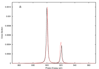
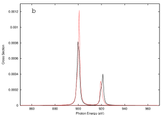
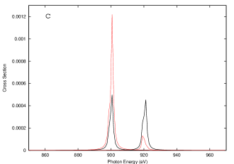
Figure 5: The scattering cross section at the $M_{\text{IV}}$ and $M_{\text{V}}$ edges for praseodymium. Each figure is for a different SIC configuration but which produces roughly the same orbital and spin moment. The thick line is for negative helicity incident x rays and the thin line is for positive helicity incident x rays: (a) Localising the $m_{l}=-1$ and $m_{l}=+1$ electrons with spin up, yields an orbital moment of $-0.07~{}\mu_{\rm B}$ and a spin moment of $2.46~{}\mu_{\rm B}$; (b) Localising the $m_{l}=-2$ and $m_{l}=+2$ electrons with spin up, yields an orbital moment of $-0.12~{}\mu_{\rm B}$ and a spin moment of $2.47~{}\mu_{\rm B}$; (c) Localising the $m_{l}=-3$ and $m_{l}=+3$ electrons with spin up, yields an orbital moment of $-0.05~{}\mu_{\rm B}$ and a spin moment of $2.52~{}\mu_{\rm B}$.

To clarify this point further, we show in Fig. 5 the cross section at the $M_{\text{IV}}$ and $M_{\text{V}}$ edges for SIC configurations that produce an orbital moment close to zero with the spins of the two occupied $f$ states parallel. While neither the spin nor the orbital moment change significantly, the cross section certainly does. At the $M_{\text{V}}$ edge the negative helicity curve is approximately constant while the positive helicity curve alters dramatically. On the other hand, at the $M_{\text{IV}}$ edge it is the positive helicity curve that is approximately constant while the negative one shows significant variation. This figure implies that the resonant x-ray scattering does not measure the total orbital moment, but is a measure of the orbital angular momentum of the individual one-electron states.

The important message of Figs. 3–5 is that the scattering cross section is not directly proportional to the total orbital moment of the material. However, both the spin and orbital moment have a strong influence on the size of the cross section peaks.

IV Discussion

The standard theory of x-ray magnetic scattering is based on the work of Blume Blum85 . He derived an equation for the nonresonant x-ray scattering cross section using a nonrelativistic approach with relativistic correction to order $1/c^{2}$. The resulting expression for the cross section, using his notation, is

$$\left(\frac{d^{2}\sigma}{d\Omega^{\prime}dE^{\prime}}\right)_{a\to b}= \left(\frac{e^{2}}{mc^{2}}\right)^{2}\delta(E_{a}-E_{b}+\hbar\omega_{k}-\hbar\omega_{k^{\prime}})$$ (38)

$$\times\left|\langle b|\sum_{j}e^{i{\bf K}\cdot{\bf r}_{j}}|a\rangle~{}{\bm{\epsilon}}^{\prime}\cdot{\bm{\epsilon}}-i\frac{\hbar\omega}{mc^{2}}~{}\langle b|\sum_{j}e^{i{\bf K}\cdot{\bf r}_{j}}\left(i\frac{{\bf K}\times{\bf P}_{j}}{\hbar k^{2}}\cdot{\bf A}+\frac{{\bf s}_{j}\cdot{\bf B}}{\hbar}\right)|a\rangle\right|^{2},$$

where $E_{a}$ and $E_{b}$ are the energies of the initial and final many-electron states, $|a\rangle$ and $|b\rangle$, respectively. ${\bf K}\equiv{\bf k}-{\bf k^{\prime}}$, where ${\bf k}$ and ${\bf k^{\prime}}$ are the wave vectors of the incoming and scattered photons, respectively, and ${\bf r}_{j}$, ${\bf P}_{j}$, and ${\bf s}_{j}$ are electron (rigorously density functional state) coordinate, momentum, and spin operators.

$${\bf A}\equiv{\bm{\epsilon}}^{\prime}\times{\bm{\epsilon}}$$ (39)

and

$${\bf B}\equiv{\bm{\epsilon}}^{\prime}\times{\bm{\epsilon}} - ({\bf{\hat{k}^{\prime}}}\times{\bm{\epsilon}}^{\prime})\times({\bf{\hat{k}}}\times{\bm{\epsilon}})$$ (40)

$$- ({\bf{\hat{k}}}\times{\bm{\epsilon}})({\bm{\epsilon}}^{\prime}\cdot{\bf{\hat{k}}})+({\bf{\hat{k}^{\prime}}}\times{\bm{\epsilon}}^{\prime})({\bm{\epsilon}}\cdot{\bf{\hat{k}^{\prime}}})$$

depend only on the direction and polarization of the incident and emitted photons. The first term in Eq. (38) is the Thomson term, responsible for the charge scattering. The term containing ${\bf A}$ depends on the orbital momentum and the term containing ${\bf B}$ depends on the electron spin. This expression clearly shows that there are three distinct contributions to the magnetic scattering cross section, one from the orbital moment, the second from the spin moment, and the third from the interference term between the spin- and orbital moment. We also note the obvious point that if the orbital and spin moments of the individual electrons sum to zero, then the magnetic scattering vanishes. Most interestingly, Eq. (38) implies that, with a suitable choice of the photon energy, geometry and photon polarization it is possible to separate contributions to the cross section from the orbital and spin moments. However, this expression is not directly applicable in our resonant magnetic scattering studies because its derivation involves an approximation which is strictly not valid close to the resonance, while our approach is only valid around resonance because we ignore the negative energy contribution to the scattering amplitude, i.e. the terms that involve creation of virtual electron-positron pairs in the intermediate states in the second order perturbation theory (see Sec. II C of Ref. Eero97, ). Another difference from Blume’s theory is the fact that our work is based on fully relativistic quantum mechanics, while Eq. (38) exploits the semi-relativistic approximation. This difference makes direct comparison of the two theories difficult. This has been discussed by Strange Stra98 who has rederived Eq. (38) as the nonrelativistic limit of a fully relativistic theory of x-ray scattering. For these reasons and the fact that there is no one-to-one correspondence between the terms in our expression for the scattering amplitude and Blume’s expression, there is no straightforward way to compare the two theories. It is often stated that Blume’s expression Eq. (38) shows that the cross section for magnetic scattering will yield the orbital and spin moment of a material separately. Although this will usually be the case it is not rigorously true. Eq. (38) cannot be applied immediately because the initial and final states $|a>$ and $|b>$ are general many-body states that have not been defined in detail. For implementation purposes they must be described as many-electron states that will contain the index $j$ which is being summed over in Eq. (38). In a magnetic material the radial part of the basis functions of the single particle wavefunctions, as well as the angular part, depend on $m_{l}$. So, we would expect the total scattering amplitude to have a contribution from the orbital angular momentum associated with each single-particle state, but this is not the same as being proportional to the total orbital angular momentum. For example a two-particle state composed of two single-particle states with $m_{l}=\pm 1$ has the same $z$-component of orbital angular momentum as a two-particle state composed of two single-particle states with $m_{l}=\pm 3$, but Eq. (38) does not suggest that they will have the same scattering amplitude. Nonetheless, Blume’s expression implies that a strong dependence of the cross section on the components of the magnetic moment is likely and indeed, this is exactly what we have found, an approximate, but by no means rigorous proportionality between orbital moment and magnitude of the cross section which is dependent on the polarization of the x ray. Furthermore, Figure 5 demonstrates explicitly the dependence of the cross section on the magnitude of $m_{l}$ of the occupied individual electron states.

The question that now arises is how our computed x-ray scattering results can be interpreted in terms of the detailed electronic structure of praseodymium. In order to understand this we analyze the electronic structure of fcc Pr for the cases where the orbital moment is equal to -4.79 $\mu_{B}$, -0.05 $\mu_{B}$, and 4.69 $\mu_{B}$ in detail. We expect the scattering cross section to reflect the Pr $f$-electron density of states. Although the shape of the cross section is partially determined by the density of states (DOS) the total DOS changes very little when pairs of electrons with differing orbital moments are localized. Therefore, a simple interpretation of the changes in the cross section with the orbital moment in terms of the total DOS cannot be made.

Figure 6: The $l=3$ contribution to the density of states of praseodymium decomposed by the $m_{j}$ quantum number for the case when the $m_{l}=-3$ and $m_{l}=-2$ $f$ states with spin up are occupied (localized). In the top right of each figure is the self-consistently calculated orbital moment. Each figure is also labelled with the relevant value of the $m_{j}$ quantum number.

In relativistic theories of magnetism different values of total angular momentum $j$ with the same $z$-component $m_{j}$ are coupled and further decomposition has little meaning Stra84 . To facilitate understanding of the differences in the spectra as orbital moment varies we show a selection of density of states curves, decomposed by the azimuthal quantum number $m_{j}$ in Figs. 6–8. There are several points that should be noted about these pictures.

Figure 7: The $l=3$ contribution to the density of states of praseodymium decomposed by the $m_{j}$ quantum number for the case when the $m_{l}=-3$ and $m_{l}=+3$ $f$ states with spin up are occupied (localized). In the top right of each figure is the self-consistently calculated orbital moment. Each figure is also labelled with the relevant value of the $m_{j}$ quantum number.

The $m_{j}=\pm 7/2$ (these are pure $j=l+1/2$ states) figures describe $f$ electron states with a well-defined $j$ value, while all the others show $f$ states with two different values of $j$ ($j=l+1/2$ and $j=l-1/2$). In all the pictures except $m_{j}=\pm 7/2$ there are two main peaks, however these two peaks do not necessarily have the same weight. The separation of the peaks represents the spin and spin-orbit splitting of the individual values of $m_{j}$. The splitting between the unoccupied $f$-states is around 0.1 Ry while the splitting between the occupied and unoccupied states is about 0.7 Ry. The smaller narrow peaks in some of these figures represent the hybridization of different $f$-states between themselves. Some of these densities of states are markedly broader than others and this is a reflection of the degree of hybridization with the conduction $s-d$ electrons.

In Fig. 6 we have chosen to apply the self-interaction corrections to the $f$-electrons which correspond to $(m_{l}=-3,m_{s}=+\frac{1}{2})$ and $(m_{l}=-2,m_{s}=+\frac{1}{2})$ (configuration 1 in Table I) in the nonrelativistic limit, and this is reflected in the density of states having a very large and narrow peak at around -0.7 Rydbergs for $m_{j}=-5/2$ and $-3/2$. There is nothing for these states to hybridize with so they are very tall and narrow atomic-like states. For $m_{j}=-5/2$ and $-3/2$ the density of states has a more band-like component corresponding to a single electronic state just above the Fermi energy. For most of the other values of $m_{j}$ there is a density of states corresponding to two electron states close to $\epsilon_{\rm F}$ and for $m_{j}=7/2$ the density of states close to $\epsilon_{\rm F}$ corresponds to a single pure $j=l+1/2$ state.

In Fig. 7 we have selected the $f$-electrons which correspond to $(m_{l}=-3,m_{s}=+\frac{1}{2})$ and $(m_{l}=+3,m_{s}=+\frac{1}{2})$ in the nonrelativistic limit for the SIC (configuration 6 in Table I). Here it is the $m_{j}=-5/2$ and the $m_{j}=+7/2$ components of the density of states that have the localized state around -0.7 Rydbergs below the Fermi energy. This means there is no $m_{j}=7/2$ character around $\epsilon_{\rm F}$ at all in this case. For most other values of $m_{j}$ we can clearly see that there are two f-states close to $\epsilon_{\rm F}$. Detailed examination of these peaks shows that the dominant cause of the splitting is the exchange field, although the splitting is also influenced by the spin-orbit interaction. For $m_{j}=-7/2$ there is only one state close to $\epsilon_{\rm F}$ of course.

Figure 8: The $l=3$ contribution to the density of states of praseodymium decomposed by the $m_{j}$ quantum number for the case when the $m_{l}=+3$ and $m_{l}=+2$ $f$ states with spin up are occupied (localized). In the top right of each figure is the self-consistently calculated orbital moment. Each figure is also labelled with the relevant value of the $m_{j}$ quantum number.

In Fig. 8 we have chosen to apply the self-interaction corrections to the $f$-electrons which correspond to $(m_{l}=+3,m_{s}=+\frac{1}{2})$ and $(m_{l}=+2,m_{s}=+\frac{1}{2})$ in the nonrelativistic limit (configuration 11 in Table I). This time it is the $m_{j}=5/2$ and $m_{j}=7/2$ states that are localized, and again there is no $m_{j}=7/2$ character around $\epsilon_{\rm F}$. The $m_{j}=-5/2$ and $m_{j}=-3/2$ state have the spin-split behaviour close to $\epsilon_{\rm F}$ in this case. The other values of $m_{j}$ behave as before.

It is clear from figures 6 to 8 that in some $m_{j}$ channels there is a small amount of band-like $f$-character below the Fermi energy. This indicates that there are two types of $f$-electron in our calculation, the localised $f$-electrons which determine the valence and the delocalised $f$-electrons which determine the valence transitions. nature It is the delocalised $f$-electrons that are principally responsible for the non-integer values of the orbital moments shown in Figures 3 and 4, (although there is also a small contribution from the valence $s-d$ electrons).

Comparison of the corresponding diagrams in Figures 6, 7, and 8 shows dramatic differences. Even though the total density of states is fairly insensitive to which $f$-electron states are occupied, the $m_{j}$-decomposed density of states is obviously drastically altered depending on which electrons are localized. In particular the $f$-states just above the Fermi energy form a significant number of the intermediate states in the formal theory described earlier. Therefore if key ones are localized they become unavailable as intermediate states for the spectroscopy and the cross section may be substantially altered. Of course, occupying one $f$-state means that some other $f$ state is not occupied which may then also play a role as an intermediate state for the spectroscopy. Indeed, how much the unavailability of particular $m_{j}$ substates affects the spectra depends on other factors too, including the $E1$ selection rules which are composed of angular matrix elements. Each angular matrix element contains four terms in the form of a product of Clebsch-Gordan coefficients and a geometry and polarization dependent factor. A further influence is the fact that the LMTO coefficients $A^{j{\bf k}}_{ti\Lambda}$ (defined in Eq. (17) and completely determined by a self-consistent band structure calculation) associated with the $f$-electrons are found to be fairly independent of the rare earth element under consideration but their magnitude has a clear but complex linear proportionality to $m_{l}$.

Detailed analysis of the major contributions to the cross section suggests that the highest peak is formed by the core-to-valence transitions $\left(d_{\frac{3}{2}},m_{j}\right)\rightarrow\left(f_{\frac{5}{2}},m_{j}+(-)1\right)$ for the $M_{\text{IV}}$ LCP(RCP) edge scattering and $\left(d_{\frac{5}{2}},m_{j}\right)\rightarrow\left(f_{\frac{7}{2}},m_{j}+(-)1\right)$ for the $M_{\text{V}}$ LCP(RCP) edge scattering. The former transition for $M_{\text{IV}}$ case is in agreement with the nonrelativistic selection rule which forbids a ${\Delta}j=2$ transition, although this transition is not totally forbidden in the relativistic $E1$ selection rule. In the $M_{\text{V}}$ case, the ${\Delta}j=0$ transition is observed to form part of the shoulder rather than contributing to the main peak. Furthermore, within the transitions forming the main peak, the contribution to the LCP scattering at both the $M_{\text{IV}}$ and $M_{\text{V}}$ edge is the largest from the most positive allowed $m_{j}$ value of the core state. On the other hand, the most negative $m_{j}$ value of the core state gives the largest contribution to the RCP scattering. This indicates the fact that the Clebsch-Gordan coefficients which are used to calculate the selection rules are a dominant factor in determining the relative size of the cross section peaks. The origin of this is simply in the properties of the Clebsch-Gordan coefficients which vary smoothly between either 0 and 1 or 0 and -1 depending on the values of the other quantum numbers.

From these considerations, we see that the separation of the LCP and RCP peaks by 1 to 2 electronvolts is a reflection of the spin-splitting of the states. In relativistic theory $m_{s}$ and $m_{l}$ are not good quantum numbers. Furthermore, because of the magnetism, different values of $j$ with the same $m_{j}$ are also coupled. However, it is still possible to associate $\langle s_{z}\rangle$, $\langle l_{z}\rangle$ with these quantum numbers and also to recognize the dominant $j$ in atomic-like unhybridized bands. For example, in the case of LCP scattering at the $M_{\text{IV}}$ edge, the largest contribution to the cross section comes from $(\kappa=3,m_{j}=+\frac{5}{2})$-like orbitals. The two 4$f$ states which have this $m_{j}$ as the main contributor are characterized by $(\langle s_{z}\rangle\simeq+\frac{1}{2},\langle l_{z}\rangle\simeq+2)$ and $(\langle s_{z}\rangle\simeq-\frac{1}{2},\langle l_{z}\rangle\simeq+3)$. Electronic structure calculation shows that the former state is dominated by $\kappa=-4$ and the latter by $\kappa=3$. Therefore the $M_{\text{IV}}$ LCP peak is most affected by the availability of the spin-down $\langle l_{z}\rangle\simeq 3$ state as an intermediate state. Similar analysis shows that the $M_{\text{IV}}$ RCP peak is most affected by spin-up $\langle l_{z}\rangle\simeq-3$ state, $M_{\text{V}}$ LCP by spin-up $\langle l_{z}\rangle\simeq 3$, and $M_{\text{V}}$ RCP by spin-down $\langle l_{z}\rangle\simeq-3$ state.

Although this analysis is a gross simplification, it does explain why the relative peak energy positions in the LCP and RCP scattering cases swap between the $M_{\text{IV}}$ and $M_{\text{V}}$ edges (see Fig. 5). Of course this is true only if these states are still available after the chosen localizations by SIC. The effect of localization on the MXRS spectrum is most dramatic if SIC is applied to these key states, changing the peak energy separation as well as the scattering amplitude between the LCP and RCP scattering cases.

Some empty valence band $f$ states participating in the scattering process have nearly equal mixture of the two $j$ characters, i.e. $j=l+1/2$ and $j=l-1/2$. If there is strong spin-up and spin-down character in the unoccupied valence states described by a specific $m_{j}$ then both spin states may be available as the intermediate states for the spectroscopy. Thus we may clearly see a two-peak structure in the $m_{j}$ decomposed amplitude for a certain polarization at the absorption edge. Figure 9 shows the core $m_{j}$ decomposed LCP scattering amplitude and the two-peak structure mentioned above is clearly visible for $m_{j}=+\frac{1}{2}$ at the $M_{\text{IV}}$ edge.

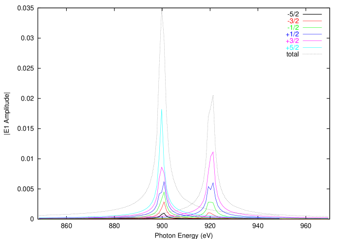
Figure 9: Core $m_{j}$ decomposed LCP amplitude at the $M_{\text{IV}}$ and $M_{\text{V}}$ edges. This figure is for the case when the $m_{l}=-3$ and $m_{l}=-2$ states are occupied.

In certain cases we can interpret the apparent relation between the magnetic cross section and the $z$-component of the total orbital moment as follows. Because $\langle l_{z}\rangle+\langle s_{z}\rangle=\langle j_{z}\rangle$ holds, then we see that if we apply self interaction corrections to states systematically according to Hund’s rules, what is effectively done is to occupy the states in order of $m_{j}$. As stated earlier the $m_{j}$ decomposed relativistic magnetic scattering cross section has a ’proportionality’ to $m_{j}$ due to the Clebsch-Gordan coefficient in the angular matrix element expression defining the $E1$ selection rules. Whether this proportionality is direct or inverse depends on the polarization of x rays. In addition, according to the electronic structure calculation, as the unhybridized state goes from $(\langle l_{z}\rangle\simeq-3,\langle s_{z}\rangle\simeq\frac{1}{2})$ to $(\langle l_{z}\rangle\simeq+3,\langle s_{z}\rangle\simeq\frac{1}{2})$, the dominant $j$ changes from $j=\frac{5}{2}$ to $j=\frac{7}{2}$ gradually. This tells us two things. Firstly we notice that if a certain state has a major impact on the scattering cross section at the $M_{\text{IV}}$ edge for RCP photons, then this same state has a relatively minor effect on the cross section for LCP photons at the same edge because of the Clebsch-Gordan factor in the expression for the $E1$ selection rules as mentioned above. Secondly we see that this same state also has only a minor effect on the $M_{\text{V}}$ cross section because the value of $j$ for the intermediate states involved in major transition differ between $M_{\text{IV}}$ and $M_{\text{V}}$.

As the SIC configuration varies from $(\langle l_{z}\rangle\simeq-3,\langle s_{z}\rangle\simeq+\frac{1}{2})$ and $(\langle l_{z}\rangle\simeq-2,\langle s_{z}\rangle\simeq+\frac{1}{2})$ to $(\langle l_{z}\rangle\simeq-3,\langle s_{z}\rangle\simeq+\frac{1}{2})$ and $(\langle l_{z}\rangle\simeq+3,\langle s_{z}\rangle\simeq+\frac{1}{2})$ so that there is a systematic change in the $z$-component of the total orbital moment, the $M_{\text{IV}}$ RCP cross section increases because the second, third and so on, strongest contributors to the cross section become additionally available as intermediate states as they are released from the SIC localization. However, they have progressively less impact as we proceed through this series of quantum numbers since the major $j$ gradually changes to $j=\frac{7}{2}$. The cross section at the $M_{\text{IV}}$ edge for LCP photons is not affected much by this change in quantum numbers since neither the initial nor the final SIC combination in the above series involves the major contributors to $M_{\text{IV}}$ LCP cross section. On the other hand, the $M_{\text{V}}$ edge LCP cross section is reduced as more and more significant contributors are removed from the available intermediate states, while the cross section at the $M_{\text{V}}$ edge for RCP photons is not much affected for the same reason as $M_{\text{IV}}$ LCP case. Obviously the above change in SIC configuration is very artificial. However as the states are filled up according to Hund’s rule as we proceed through the rare earth series, we would expect to observe changes in the cross section governed by these considerations for rare earths where the intermediate states can be considered as atomic-like. However, a very different interpretation of the x-ray spectra may be required in the case where delocalized band-like intermediate states are of primary importance, as is the case in resonant x-ray scattering at the $K$ and $L_{\text{II,III}}$ edges.

Finally, we are unaware of any experimental measurements of the MXRS spectra of praseodymium or it compounds at the $M_{\text{IV}}$ or $M_{\text{V}}$ edge. However a careful combined neutron Goff and x-ray Vig (at the $L_{\text{II,III}}$ edges) investigation into the magnetism of Ho_xPr_1-x alloys has concluded that the Pr ion does have a 4$f$ moment at all values of $x$. Deen et al. Pascal02 have performed MXRS measurements at the $L$ edges in Nd/Pr superlattices and found a large peak at the absorption edge and a high energy shoulder corresponding to dipolar transitions to the broad 5$d$ band. We hope that our calculations will stimulate detailed experimental x-ray studies of $M_{\text{IV}}$ and $M_{\text{V}}$ edges of Pr, in pure Pr and in its alloys and compounds.

V Conclusions

In conclusion, a theory of magnetic x-ray scattering that is based on the LSD with self-interaction corrections and second order time-dependent perturbation theory has been described. We have illustrated the theory with an application to fcc praseodymium and used this example to illustrate the dependence of the scattering cross section on spin and orbital magnetic moments. It has been shown that the theory quantitatively reproduces the dependence on the spin and orbital magnetic moments originally predicted qualitatively Blum85 .

VI acknowledgements

P. S. and E. A. would like to thank the British EPSRC for research grant (number GR/M45399/01) during which the bulk of the work reported in this paper was carried out. M. H. would like to thank Keele University for a Ph.D studentship. E. A. is also indebted to Tampere City Science Foundation for a grant to cover some personal research expenses.

References

• (1) M. Blume, J. Appl. Phys. 57, 3615 (1985).
• (2) M. Blume and D. Gibbs, Phys. Rev. B 37, 1779 (1988).
• (3) J. P. Hannon, G. T. Trammell, M. Blume, and D. Gibbs, Phys. Rev. Lett. 61, 1245 (1988).
• (4) A. Fasolino, P. Carra and M. Altarelli, Phys. Rev. B 47, 3877 (1993).
• (5) P. Rennert, Phys. Rev. B 48, 13 559 (1993).
• (6) S. W. Lovesey, K. S. Knight, and E. Balcar, Phys. Rev. B 64, 054405 (2001); S. W. Lovesey, K. S. Knight, and D. S. Sivia, Phys. Rev. B 65, 224402 (2002); S. W. Lovesey, J. Phys. Condens. Matter 14, 4415 (2002).
• (7) M. Takahashi, J. Igarashi, and P. Fulde, Journal of the Physical Society of Japan 69, 1614 (2000), and references therein.
• (8) P. Hohenberg and W. Kohn, Phys. Rev. 136, B864 (1964); W. Kohn and L. J. Sham, Phys. Rev. A 140, 1133 (1965).
• (9) W. Kohn and P. Vashishta, in Theory of the Inhomogeneous Electron Gas, edited by S. Lundqvist and N. H. March (Plenum Press, New York,1982).
• (10) E. Arola, P. Strange and B. L. Gyorffy, Phys. Rev. B 55, 472 (1997).
• (11) E. Arola and P. Strange, Appl. Phys. A 73, 667 (2001).
• (12) E. Arola, P. Strange, N. I. Kulikov, M. J. Woods, and B. L. Gyorffy, J. Magn. Magn. Mater. 177-181 1415 (1998); E. Arola and P. Strange, Phys. Rev. B 58, 7663 (1998).
• (13) V. Anisimov, F. Aryasetiawan, and A. I. Lichtenstein, J. Phys. Condens. Matter 9, 767 (1997).
• (14) M. Arai and T. Fujiwara, Phys. Rev. B 51, 1477 (1995).
• (15) Z. Szotek, W. M. Temmerman, and H. Winter, Phys. Rev. B 47, 4029 (1993).
• (16) W. M. Temmerman, A. Svane, Z. Szotek and H. Winter, in Electronic Density Functional Theory: Recent Progress and New Directions, edited by J. F. Dobson, G. Vignale, and M. P. Das (Plenum, 1997).
• (17) A. Svane and O. Gunnarsson, Phys. Rev. Lett. 65, 1148 (1990).
• (18) P. Strange, A. Svane, W. M. Temmerman, Z. Szotek, and H. Winter, Nature 399, 756 (1999).
• (19) S. V. Beiden, W. M. Temmerman, Z. Szotek, and G. A. Gehring, Phys. Rev. Lett. 79, 3970 (1997).
• (20) F. E. Low, Phys. Rev. 96, 1428 (1954); M. Gell-Mann and M. L. Goldberger, ibid. 96, 1433 (1954).
• (21) P. M. Platzman and N. Tzoar, Phys. Rev. B 2, 3556 (1970).
• (22) D. Gibbs, D. R. Harshman, E. D. Isaacs, D. B. McWhan, D. Mills, and C. Vettier, Phys. Rev. Lett. 61, 1241 (1988).
• (23) The Xmas beamline at the European Synchrotron Radiation Facility, for example.
• (24) W. G. Stirling and M. J. Cooper, J. Magn. Magn. Mater. 200, 755 (1999).
• (25) M. J. Cooper and W. G. Stirling, Radiation Physics and Chemistry 56, 85 (1999).
• (26) F. Borgatti, G. Ghiringhelli, P. Ferriani, G. van der Laan, and C. M. Bertoni, Phys. Rev. B, 69, 134420, (2004).
• (27) P. Carra and B. T. Thole, Reviews of Modern Physics 66, 1509 (1994).
• (28) J. Luo, G.T. Trammell and J.P. Hannon, Phys. Rev. Lett. 71, 287 (1993).
• (29) P. J. Durham, in Electronic Structure of Complex Systems, edited by P. Phariseau and W. M. Temmerman, Vol. 113 of NATO Advanced Study Institute, Series B: Physics (Plenum Press, New York, 1984).
• (30) O. K. Andersen and O. Jepsen, Phys. Rev. Lett. 53, 2571 (1984); O. K. Andersen, O. Jepsen, and O. GlΓΆtzel, Canonical Description of the Band Structures of Metals, Proc. of Int. School of Physics, Course LXXXIX, Varenna, 1985, edited by F. Bassani, F. Fumi, and M. P. Tosi (North-Holland, Amsterdam, 1985), p. 59; H. L. Skriver, The LMTO Method, Springer series in Solid State Sciences Volume 41, (Springer-Verlag, 1984); I. Turek, V. Drchal, J.Kudrnovsky, M. Sob, and P. Weinberger, Electronic Structure of Disordered Alloys, Surfaces and Interfaces, (Kluwer Academic Publishers, 1997).
• (31) J. P. Perdew and A. Zunger, Phys. Rev. B 23, 5048 (1981).
• (32) A. Svane, Phys. Rev. B 51, 7924 (1995).
• (33) A. Svane and O. Gunnarsson, Phys. Rev. B 37, 9919 (1988); A. Svane and O. Gunnarsson, Europhys. Lett. 7, 171 (1988).
• (34) J. A.Β Majewski and P.Β Vogl, Phys. Rev. B 46, 12219 (1992); ibid. 46, 12235 (1992).
• (35) A. Svane, Phys. Rev. Lett. 68, 1900 (1992).
• (36) W. M. Temmerman, Z. Szotek, and H. Winter, Phys. Rev. B 47, 1184 (1993).
• (37) L. Petit, A. Svane, Z. Szotek, and W. M. Temmerman, Science 301, 498 (2003).
• (38) R. Tyer, W. M. Temmerman, Z. Szotek, G. Banach, A. Svane, L. Petit, and G. A. Gehring, Europhys. Lett. 65, 519 (2004)
• (39) W. M. Temmerman, H. Winter, Z. Szotek, and A. Svane, Phys. Rev. Lett. 86, 2435 (2001).
• (40) A. Svane and O. Gunnarsson, Solid State Commun. 76, 851 (1990).
• (41) P. Strange, Relativistic Quantum Mechanics, with applications in condensed matter and atomic physics (Cambridge University Press, 1998).
• (42) W. M.Temmerman, A. Svane, Z.Szotek, H. Winter, and S. V. Beiden, ”On the implementation of the Self-Interaction Corrected Local Spin Density Approximation for $d$- and $f$-electron systems”, Lecture notes in Physics 535: Electronic Structure and Physical properties of Solids: The uses of the LMTO method Edited by H. Dreysse, p. 286, (Springer-Verlag, Berlin, 2000).
• (43) H. Ebert, Phys. Rev. B 38, 9390 (1988).
• (44) H. Ebert, P. Strange and B. L. Gyorffy, J. Appl. Phys. 63, Part 2, 3052 (1988).
• (45) P.Strange, J. B. Staunton and B. L. Gyorffy, J. Phys. C 17, 3355 (1984).
• (46) Our definition of the scattering amplitude [$f^{(\text{our})}(\omega)$] differs slightly from the standard one [$f^{(\text{std})}(\omega)$] defined by the differential scattering cross section $d\sigma/d\Omega=\left|f^{(\text{std})}(\omega)\right|^{2}$. They are connected by the relation $f^{(\text{std})}(\omega)=f^{(\text{our})}(\omega)V\omega/(2\pi\hbar c^{2})$ [see Sec. III A and Ref. 25 in Ref.Β Eero97, ].
• (47) M. E. Rose, Relativistic Electron Theory, (John Wiley, New York, 1971).
• (48) E. Arola The Relativistic KKR-CPA Method: A Study of Electronic Structures of Cu75Au25, Au70Pd30, and Cu75Pt25 Disordered Alloys, Acta Polytechnica Scandinavica, Applied Physics Series No. 174, Edited by M. Luukkala (The Finnish Academy of Technology, Helsinki, 1991).
• (49) H. L. Skriver, The LMTO Method (Springer Verlag, Heidelberg, 1984).
• (50) Single-site solutions of the Dirac equation with magnetic field do not have well-defined angular momentum character, and only $m_{j}$ remains as a good quantum number (cf. Eq. (13) of Ref.Β Eero97, ).
• (51) E. Bucher, C. W. Chu, J. P. Maita, K. Andres, A. S. Cooper, E. Buehler, and K. Nassau, Phys. Rev. Lett. 22, 1260 (1969).
• (52) A. Yu. Kutznetsov, V. P. Dmitriev, O. I. Bandilet and H. P. Weber, Phys. Rev. B 68, 064109 (2003).
• (53) H. W. Myron and S. H. Liu, Phys. Rev. B 1, 2414 (1970).
• (54) P. SΓΆderlind, Phys. Rev. B 65, 115105 (2002).
• (55) A. Svane, J. Trygg, B. Johansson, and O. Eriksson, Phys. Rev. B 56, 7143 (1997).
• (56) P. Strange, M. Horne, Z. Szotek, W. M. Temmerman and H. Ebert, unpublished.
• (57) J. P. Goff, C. Bryn-Jacobsen, D. F. McMorrow, G. J. McIntyre, J. A. Simpson, R. C. C. Ward, and M. R. Wells, Phys. Rev. B 57, 5933 (1998).
• (58) A. Vigliante, M. J. Christensen, J. P. Hill, G. Helgesen, S. A. Sorensen, D. F. McMorrow, D. Gibbs, R. C. C. Ward, and M. R. Wells, Phys. Rev. B 57, 5941 (1998).
• (59) P. P. Deen, J. P. Goff, R. C. C. Ward, M. R. Wells, and A. Stunault, J. Magn. Magn. Mater. 240, 553 (2002).