The Effect of Columnar Disorder on the Superconducting Transition of a Type-II Superconductor in Zero Applied Magnetic Field

Abstract

We investigate the effect of random columnar disorder on the superconducting phase transition of a type-II superconductor in zero applied magnetic field using numerical simulations of three dimensional XY and vortex loop models. We consider both an unscreened model, in which the bare magnetic penetration length is approximated as infinite, and a strongly screened model, in which the magnetic penetration length is of order the vortex core radius. We consider both equilibrium and dynamic critical exponents. We show that, as in the disorder free case, the equilibrium transitions of the unscreened and strongly screened models lie in the same universality class, however scaling is now anisotropic. We find for the correlation length exponent $\nu=1.2\pm 0.1$, and for the anisotropy exponent $\zeta=1.3\pm 0.1$. We find different dynamic critical exponents for the unscreened and strongly screened models.

I Introduction

The discovery of high temperature superconductors, in which thermal fluctuations are important and mean field theory can no longer be applied, has led to a resurgence of interest in phase transitions and critical phenomena in type-II superconductors.Blatter Of particular interest has been understanding the effects of random quenched disorder on the nature of the ordered phases and the universality of the phase transitions. For the high temperature superconductors, this quenched disorder can take many forms: random point defects due to oxygen vacancies, planar twin grain boundaries, and columnar defects introduced by ion irradiation.

Most of the work in this area has focused on the case of a finite applied magnetic field, where one seeks to understand how the randomness distorts or destroys the Abrikosov lattice of magnetic field induced vortex lines that forms in a pure system. Columnar defectsNelson ; Wallin1 ; Wallin2 have received considerable attention, as they are particularly effective in pinning vortex lines and reducing flux flow resistance. In contrast, in this paper we will focus on the effect of columnar defects on the superconducting phase transition in zero applied magnetic field. We expect this case to be interesting for the following reason. A generalized Harris criterionWallin3 ; Chayes ; Harris argues that disorder will be a relevant perturbation, and change the universality class of a phase transition, whenever $2-d^{*}\nu>0$, where $d^{*}$ is the number of dimensions in which the system is disordered, and $\nu$ is the usual correlation length critical exponent. For a disorder free superconductor, the transition in zero applied magnetic field is in the universality class of the three dimensional (3D) XY model,Dasgupta for which $\nu\gtrsim 2/3$. For random point disorder, $d^{*}=3$, so $2-d^{*}\nu<0$, and the generalized Harris criterion argues that the universality of the transition remains unchanged. For columnar disorder, however, $d^{*}=2$, and so $2-d^{*}\nu>0$. Columnar defects should therefore cross the zero field transition over to a new universality class. StabilityChayes of this new disordered fixed point with respect to the generalized Harris criterion implies that it should have a new value $\nu>1$. In our equilibrium simulations we indeed find behavior consistent with this, and we obtain a value for the correlation length exponent $\nu=1.2\pm 0.1$. Moreover, we find scaling is now anistropic and we find the value of the anisotropy exponent to be $\zeta=1.3\pm 0.1$. Experimental measurement of these exponents would therefore provide a precision test of the theoretical model.

The model we study also has application to the $T=0$ superconductor to insulator quantum phase transition in two dimensional thin films with random substrate disorder,Wallin3 ; Cha ; Svistunov and to the Mott transition for bosons in 2D optical lattices with the addition of random scattered laser intensity. optical In these cases, the two dimensional quantum problem can be mapped onto a corresponding three dimensional classical problem with the same symmetries as the one we study here.Sachdev

To study the effect of columnar disorder on the zero field transition of a type-II superconductor, we will consider two different limits. The first is the limit of an “unscreened” superconductorWallin2 ; Teitel in which magnetic field fluctuations are frozen out, corresponding to the approximation of an infinite bare magnetic penetration length, $\lambda_{0}\to\infty$. Here, vortex line segments have long ranged Coulombic-like interactions. For the extreme type-II high temperature superconductors, for which $\kappa\equiv\lambda_{0}/\xi_{0}\sim 100$, where $\xi_{0}$ is the bare coherence length that also sets the radius of a vortex line core, the unscreened model should give a good description except in an extremely narrow temperature window about the transition.Fisher

The second limit is that of a strongly screened superconductor,Wallin1 ; Wallin4 corresponding to the case $\lambda_{0}\sim\xi_{0}$. In this case, vortex line segments have short range interactions. This description should also become valid extremely close to the transition when the diverging correlation length $\xi$ becomes comparable to the renormalized magnetic penetration length $\lambda$, $\lambda\lesssim\xi$, and magnetic field fluctuations on such large length scales must be included in determining the true critical behavior. This region near $T_{c}$ may, however, be too small to observe in practice.Fisher

As in the disorder free case, a duality transformationDasgupta ; Kleinert ; Savit establishes that these two limits lie in the same universality class as regards equilibrium critical behavior. They may be different, however, for dynamic critical behavior.Wallin4 In this work we carry out detailed Monte Carlo (MC) simulations of the XY model for the unscreened superconductor to determine the equilibrium critical exponents, and we demonstrate the presence of anisotropic scaling; by duality, these exponents also apply to the strongly screened case. Then, using simple local Monte Carlo dynamics, we compute the dynamic critical exponent for both the unscreened XY model, and for the strongly screened vortex loop model. We find that the dynamic exponent is different for these two limits.

The remainder of this paper is organzied as follows. In Section II we describe the XY model and the loop model for the unscreened and strongly screened limits, respectively. The duality transformation between the two is given in Appendix A. In Section III we discuss the equilibrium critical behavior of the XY model, presenting our finite size scaling analysis, defining the observables we measure, and giving the numerical results of our simulations. In Section IV we discuss the dynamic critical behavior of the XY and loop models, within a simple local Monte Carlo dynamics. We define the observables we measure and give our numerical results. In Section V we give our discussion and conclusions.

II Models

II.1 XY Model

To model the effects of thermal fluctuations in a type-II superconductor, we start with the commonly used 3D XY model.Teitel This models the phase fluctuations of the superconducting order parameter in the “unscreened” limit where magnetic field fluctuations are frozen out, corresponding to the approximation of an infinite bare magnetic penetration length, $\lambda_{0}\to\infty$. For zero applied magnetic field we have,

$${\cal H}_{\rm XY}[\theta_{i}]=-\sum_{i,\mu}J_{i\mu}\cos(\theta_{i}-\theta_{i+\hat{\mu}})\enspace.$$ (1)

Here $\theta_{i}$ represents the phase angle of the complex superconducting order parameter on node $i$ of a periodic cubic grid of $N=L\times L\times L_{z}$ sites, with periodic boundary conditions in all directions. The sum is over all nearest neighbor bonds $(i,\mu)$ of the grid, with $\hat{\mu}=\hat{x},\hat{y},\hat{z}$, and the cosine term represents the kinetic energy of fluctuating supercurrents. The short length cutoff of the discrete grid models the bare vortex core size $\xi_{0}$.

In a pure system, the couplings $J_{i\mu}$ are all equal, except for a possible variation with bond direction $\mu$. Here, we take the $J_{i\mu}$ randomly distributed in order to model quenched random columnar defects. For the work reported on here, with columnar defects aligned parallel to the $\hat{z}$ axis, we have chosen the following distribution: in the $\hat{z}$ direction, we take all $J_{iz}=1$; in the $xy$ plane, we take $J_{i\mu}$, $\mu=x,y$, distributed equally likely with the two values $0.1$ and $1.9$, keeping the $J_{i\mu}$ translationally invariant along the $\hat{z}$ axis so as to model columnar disorder. Note that the random $J_{i\mu}$ introduce no frustration into the system; in the ground state all the $\theta_{i}$ are equal. The variations in the $J_{i\mu}$ result in spatially random pinning energies for vortex loop excitations of the phase angles $\theta_{i}$. We have chosen the above bimodal distribution for $J_{i\mu}$ to give strong pinning energies (for fixed average $J_{i\mu}$), so as to be able to approach the asymptotic scaling limit with reasonable size systems.

Although we will simulate the Hamiltonian of Eq.(1) using periodic boundary conditions on the phase angles $\theta_{i}$, it is useful to consider a more general fixed twist boundary condition,

$$\theta_{i+L_{\mu}\hat{\mu}}=\theta_{i}+\Delta_{\mu}\enspace,$$ (2)

where $\Delta_{\mu}$ is a fixed (non-fluctuating) total twist in the phase angle applied across the system in direction $\hat{\mu}$. Periodic boundary conditions correspond to the twist $\Delta_{\mu}=0$. Transforming to new variables,

$$\theta^{\prime}_{i}=\theta_{i}-(\Delta_{\mu}/L_{\mu}){\bf r}_{i}\cdot\hat{\mu}\enspace,$$ (3)

the Hamiltonian of Eq.(1) becomes,

$${\cal H}_{\rm XY}[\theta_{i}^{\prime};\Delta_{\mu}]=-\sum_{i,\mu}J_{i\mu}\cos(\theta^{\prime}_{i}-\theta^{\prime}_{i+\hat{\mu}}-\Delta_{\mu}/L_{\mu})\enspace,$$ (4)

where the $\theta^{\prime}_{i}$ obey periodic boundary conditions, $\theta^{\prime}_{i+L_{\mu}\hat{\mu}}=\theta^{\prime}_{i}$. Using the fact that the cosine is periodic in $2\pi$, the partition function integrals over $\theta_{i}^{\prime}$ can be taken over the interval $\theta_{i}^{\prime}\in[0,2\pi)$, as were the integrals over the original phase angles $\theta_{i}$. Considering how the free energy varies with the twist $\Delta_{\mu}$ will be useful later for discussing phase coherence in the model.

II.2 Loop Model

Although we carry out our equilibrium simulations directly in terms of the XY model of Eq.(1), we also consider a different formulation of the model. If instead of the cosine interaction of Eq.(1), one uses the periodic Gaussian interaction of Villain,Villain then a standard duality transformationDasgupta ; Kleinert ; Savit (see Appendix A) maps the XY model, ${\cal H}_{\rm XY}/T$, onto a model of sterically interacting loops, ${\cal H}_{\rm loop}/\tilde{T}$, where,

$${\cal H}_{\rm loop}={1\over 2}\sum_{i,\mu}g_{i\mu}n_{i\mu}^{2}\enspace.$$ (5)

The $n_{i\mu}$ are integer valued variables on the bonds $(i,\mu)$ and satisfy a divergenceless constraint,

$$\sum_{i,\mu}\left[n_{i\mu}-n_{i-\hat{\mu},\mu}\right]=0\enspace.$$ (6)

The $n_{i\mu}$ thus form connected paths through the system that must eventually close upon themselves. The couplings $g_{i\mu}$ of Eq.(5) are related to the couplings of the XY model by,

$$g_{i\mu}/\tilde{T}=T/J_{i\mu}\enspace,$$ (7)

where the temperature scale of the loop model, $\tilde{T}$, is inverted with respect to the temperature scale of the XY model, $T$.

While the loop model of Eq.(5) is exactly dual to the XY model of an unscreened superconductor, taking it on its own with $\tilde{T}$ as the physical temperature, we can give ${\cal H}_{\rm loop}$ the following different physical interpretation.Wallin1 ; Wallin4 We can regard the divergenceless variables $n_{i\mu}$ as the vortex loops of a strongly screened superconductor with $\lambda_{0}\sim\xi_{0}$. The short ranged vortex line interaction of this case is then modeled by the simple onsite repulsion of ${\cal H}_{\rm loop}$. Further details of this analogy may be found in Ref.Wallin4, . If we regard each site of our numerical grid as representing a columnar pin, the random $g_{i\mu}$ in the $xy$ plane can be thought of as modeling the random distances between such pins, and hence giving the random energies associated with a vortex loop segment hopping from one pin to another. This duality between ${\cal H}_{\rm loop}$ and ${\cal H}_{\rm XY}$ thus implies that the unscreened and the screened superconductor models fall in the same equilibrium universality class, just as is the case for the disorder free model.Dasgupta

III Equilibrium Critical Behavior

In this section we report on our equilibrium XY model simulations. To extract critical exponents, we use the method of finite size scaling. We first, therefore, discuss this method.

III.1 Finite Size Scaling

Because the columnar disorder singles out the special direction $\hat{z}$, we must allow for the possibility that scaling will be anisotropic. If $\xi$ denotes the correlation length in the $xy$ plane, then anisotropic scaling assumes that, as $T\to T_{c}$ and $\xi$ diverges, the correlation length along the $\hat{z}$ axis diverges as,

$$\xi_{z}\sim\xi^{\zeta}\enspace,$$ (8)

where $\zeta$ is the anisotropy exponent.

Consider now an observable ${\cal O}$ whose scaling dimension is zero. As a function of reduced temperature $t\equiv(T-T_{c})/T_{c}$ and system size $L\times L\times L_{z}$, we expect the scaling relationship,

$${\cal O}(T,L,L_{z})=\tilde{\cal O}(tb^{1/\nu},L/b,L_{z}/b^{\zeta})\enspace,$$ (9)

where $b$ is an arbitrary length rescaling factor, $\tilde{\cal O}$ is the scaling function, and $\nu$ is the usual correlation length exponent,

$$\xi\sim t^{-\nu}\enspace.$$ (10)

Taking $b=L$ in Eq,(9) then gives,

$${\cal O}(T,L,L_{z})=\tilde{\cal O}(tL^{1/\nu},1,L_{z}/L^{\zeta})\enspace.$$ (11)

For the case of isotropic scaling, with $\zeta=1$, choosing a constant aspect ratio $L_{z}=\gamma L$ reduces the right hand side of Eq.(11) to a function of the single scaling variable $tL^{1/\nu}$. Measuring ${\cal O}$ vs. $T$ for systems with varying $L$ but fixed $L_{z}/L$ is then sufficient to determine the exponent $\nu$. However when $\zeta\neq 1$, and its value is unknown, it becomes necessary to consider systems with varying aspect ratio $L_{z}/L$, greatly increasing the complexity of the computation.

To deal with this case we take the following approach, originally used to study the phase transition in the quantum Ising spin glass.Young Assume that the observable ${\cal O}(T,L,L_{z})$ when viewed as a function of $L_{z}$, for fixed $T$ and $L$, has a maximum at a particular value $L_{z\,{\rm max}}$. Because of the scaling law Eq.(11), this value $L_{z\,{\rm max}}$ must occur when

$$L_{z\,{\rm max}}/L^{\zeta}=\tilde{\gamma}(tL^{1/\nu})\enspace,$$ (12)

where $\tilde{\gamma}$ is a scaling function of the single variable $tL^{1/\nu}$. We then define,

$${\cal O}_{\rm max}(T,L)\equiv{\cal O}(T,L,L_{z\,{\rm max}})=\tilde{\cal O}(tL^{1/\nu},1,\tilde{\gamma}(tL^{1/\nu}))\equiv\tilde{\cal O}_{\rm max}(tL^{1/\nu})\enspace.$$ (13)

Plotting ${\cal O}_{\rm max}(T,L)$ vs. $T$ for different values of $L$, the curves will intersect at the common point $T=T_{c}$ (i.e. $t=0$). The slopes of these curves at $T_{c}$ then determine the exponent $\nu$. In practice, we will determine the values of $T_{c}$ and the exponent $\nu$ by the following approach.Nightingale Close to $T_{c}$ (i.e for small $t$) we can expand the scaling function $\tilde{\cal O}_{\rm max}$ as a polynomial for small values of its argument $tL^{1/\nu}$,

$$\tilde{\cal O}_{\rm max}(tL^{1/\nu})\simeq a_{0}+a_{1}[(T-T_{c})/T_{c}]L^{1/\nu}+a_{2}\left([(T-T_{c})/T_{c}]L^{1/\nu}\right)^{2}+\dots$$ (14)

We then fit the data for ${\cal O}_{\rm max}(T,L)$ to the above form using $T_{c}$, $\nu$, $a_{0}$, $a_{1}$, $a_{2}\dots$ as free fitting parameters. Varying the system sizes $L$ and temperature window $|T-T_{c}|$ of the data used in the fit, as well as varying the order of the above polynomial expansion, will give confidence on the significance of the fit.

Having obtained the value of $T_{c}$, plotting $L_{z\,{\rm max}}(T_{c})$ vs. $L$ determines the anisotropy exponent $\zeta$ by Eq.(12),

$$L_{z\,{\rm max}}(T_{c})\sim L^{\zeta}\enspace.$$ (15)

Knowing $T_{c}$, $\nu$ and $\zeta$, plotting ${\cal O}_{\rm max}(T,L)$ vs. $tL^{1/\nu}$ and ${\cal O}(T_{c},L,L_{z})$ vs. $L_{z}/L^{\zeta}$ should collapse the respective data to a single scaling curve.

III.2 Observables

To carry out the scaling analysis outlined in the previous section, we now have to determine appropriate observables to measure.

For the 3D XY model of Eq.(1), we expect below $T_{c}$ a non-vanishing order parameter, $\psi=(1/N)\sum_{i}{\rm e}^{i\theta_{i}}$. We define the real part of $\psi$ as,

$$M={1\over N}\sum_{i}\cos\theta_{i}\enspace,$$ (16)

and construct its Binder ratioBinder

$$g(T,L,L_{z})\equiv 1-\left[{\langle M^{4}\rangle\over 3\langle M^{2}\rangle^{2}}\right]=\tilde{g}(tL^{1/\nu},L_{z}/L^{\zeta})\enspace.$$ (17)

Because the scaling dimension of $M$ cancels in taking the ratio above, the Binder ratio $g$ has scaling dimension zero, and so has the scaling form of Eq.(11). In the above, $\langle\dots\rangle$ denotes the usual thermal average, while $[\dots]$ denotes the average over different realizations of the columnar disorder. In the denominator of Eq.(17), the square of the expectation value is evaluated using two replicas with identical disorder, indexed by $a$ and $b$, $\langle M^{2}\rangle^{2}\equiv\langle(M^{a})^{2}\rangle\langle(M^{b})^{2}\rangle$, in order to avoid bias.Olson

Another observable we have measured is obtained by considering the dependence of the total free energy on the total applied twist across the system.Reger Sensitivity to boundary conditions, in this case specified by the twist $\Delta_{\mu}$ in Eq.(2), is one of the signatures of an ordered phase. The XY model is therefore phase coherent when the total free energy ${\cal F}$ varies with twist $\Delta_{\mu}$. ${\cal F}$ is computed from a partition function sum over the $\theta_{i}^{\prime}$ using the Hamiltonian ${\cal H}_{\rm XY}[\Delta_{\mu}]$ of Eq.(4). A convenient measure of the dependence of ${\cal F}$ on $\Delta_{\mu}$ is obtained by looking at the curvature of ${\cal F}(\Delta_{\mu})$ at its minimum. In Appendix A we show that this minimum always occurs at $\Delta_{\mu}=0$. We therefore consider,

$$\left.{\partial^{2}{\cal F}\over\partial\Delta_{\mu}^{2}}\right|_{\Delta_{\mu}=0}=\left\langle{\partial^{2}{\cal H}_{\rm XY}\over\partial\Delta_{\mu}^{2}}\right\rangle-{1\over T}\left\langle\left({\partial{\cal H}_{\rm XY}\over\partial\Delta_{\mu}}\right)^{2}\right\rangle\enspace,$$ (18)

where ${\cal H}_{\rm XY}$ is that of Eq.(4), and the averages on the right hand side are taken in the ensemble with $\Delta_{\mu}=0$.

Since the total free energy ${\cal F}$ and the total twist $\Delta_{\mu}$ are both scale invariant quantities, then $\partial^{2}{\cal F}/\partial\Delta_{\mu}^{2}$ has scaling dimension zero. These derivatives are usually defined in terms of the helicity modulusTeitel $\Upsilon_{\mu}$, which is the derivative of the free energy density with respect to the twist per length. We have in three dimensions,

$$\left.{\partial^{2}{\cal F}\over\partial\Delta_{z}^{2}}\right|_{\Delta_{\mu}=0} = {L^{2}\over L_{z}}\Upsilon_{z}\enspace,$$ (19)

$$\left.{\partial^{2}{\cal F}\over\partial\Delta_{x}^{2}}\right|_{\Delta_{\mu}=0} = L_{z}\Upsilon_{x}\enspace.$$ (20)

Averaging over the disorder, we find that, for fixed $T$ and $L$, $(L^{2}/L_{z})[\Upsilon_{z}]$ decreases monotonically as $L_{z}$ increases, while $L_{z}[\Upsilon_{x}]$ increases monotonically as $L_{z}$ increases. In order to have an observable which has a maximum as a function of $L_{z}$, we therefore consider the product,

$$L^{2}[\Upsilon_{x}\Upsilon_{z}]=\tilde{u}(tL^{1/\nu},L_{z}/L^{\zeta})\enspace,$$ (21)

which has the same scaling form as Eq.(11).

III.3 Monte Carlo Methods and Error Estimation

In order to achieve accurate results, averaging over many disorder realizations for many different aspect ratios, $L_{z}/L$, it is essential to have an efficient simulation algorithm. For equilibrium simulation of the 3D XY model, the lack of frustration allows us to use the WolffWolff cluster algorithm to avoid critical slowing down. We typically use 100 Wolff sweeps to approach equilibrium, followed by 200 Wolff sweeps to compute averages; one Wolff sweep is defined as building clusters until each phase angle $\theta_{i}$ has been updated once on average. Between $3000$ and $5000$ different realizations of the random disorder are averaged over near the critical point, with fewer realizations used away from the critical point. A test of the equilibration of our simulations is shown in Fig. 1, where we see that the above simulation lengths are sufficient.

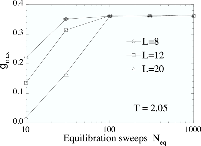
Figure 1: Binder ratio maximum for the 3D XY model, $g_{\rm max}$ at $T=2.05\simeq T_{c}$, computed with $N_{\rm eq}$ equilibration sweeps followed by $N_{\rm eq}$ sweeps to compute averages. $N_{\rm eq}=100$ is sufficient for good equilibration for all sizes $L$.

To estimate the statistical error in our results we use the following method. For our raw data, our average is just the average over the individual values obtained in $N_{d}$ independent realizations of the random disorder. Our estimated error is determined from the standard deviation $\sigma$ of these $N_{d}$ independent values, ${\rm error}=\sigma/\sqrt{N_{d}}$. To estimate the statistical error in the fitting parameters of our finite size scaling analysis, we take the following approach. From our original data set we construct many (typically $1000$) fictitious data sets by adding to each data point a random Gaussian variable with zero mean, and standard deviation equal to the estimated statistical error of the data point. We then fit each of the fictitious data sets. The standard deviation of the values of the resulting fitting parameters then gives our estimate of the statistical error in the fitting parameter.

Harder to estimate are the possible systematic errors in our results. Here we rely on varying parameters of our analysis, such as the order of a polynomial fit, or the system sizes $L$ used in the fit, in order to get a feeling for the likely accuracy of our results.

III.4 Results

We now present our results from simulations of the XY model of Eq.(1). In Fig. 2 we plot our results for the Binder ratio of Eq.(17), $g(T,L,L_{z})$ vs. $L_{z}$, for sizes $L=8,12,20$, at the fixed temperature $T=2.05$. We see that for each $L$, $g(T,L,L_{z})$ has a clear maximum at a particular $L_{z\,{\rm max}}$. Note that the maximum values of these curves appear to be equal for the different values of $L$. From Eq.(13) we therefore infer that the temperature $T=2.05$ is approximately the critical temperature $T_{c}$. To determine the precise values of $L_{z\,{\rm max}}$ and the maximum values $g_{\rm max}(T,L)=g(T,L,L_{z\,{\rm max}})$, we fit the data for each $L$ to a cubic polynomial in $\ln L_{z}$ (these are the solid curves in Fig. 2). The $L_{z\,{\rm max}}$ obtained this way are not, in general, integer values. We have also done such fits using a quadratic polynomial in $\ln L_{z}$; the difference in values obtained from the cubic vs. the quadratic fit provides our estimate of the systematic error of this procedure. We find that for $g_{\rm max}(T,L)$ this systematic error is always smaller than the estimated statistical error of the cubic fits; for $L_{z\,{\rm max}}$ the systematic error is bigger. This reflects the simple fact that $g(T,L,L_{z})$, being a maximum with zero slope, varies only quadratically with deviations from the true $L_{z\,{\rm max}}$, and hence may be determined more accurately. Henceforth, the error bars we use for $g_{\rm max}$ are the above estimated statistical errors, while the error bars we use for $L_{z\,{\rm max}}$ are the above defined systematic errors.

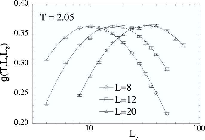
Figure 2: Binder ratio, $g(T,L,L_{z})$ vs. $L_{z}$ for several values $L$ at the fixed $T=2.05$. Solid curves are cubic polynomial fits in $\ln L_{z}$.

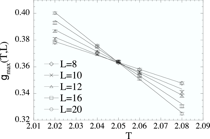
Figure 3: Binder ratio maximum $g_{\rm max}(T,L)$ vs. $T$ for various system sizes $L$. The common intersection determines $T_{c}\simeq 2.05$. Solid lines are linear fits to the data.

Proceeding in this way at other temperatures, we plot in Fig. 3 the values of $g_{\rm max}(T,L)$ vs. $T$ for $L=8$, $10$, $12$, $16$ and $20$. The different curves all intersect at a common point, determining $T_{c}\simeq 2.05$. To determine the correlation length exponent $\nu$, and get a more precise estimate of $T_{c}$, we now fit the data of Fig. 3 to a polynomial expansion as in Eq.(14). In Table 1 we show the results from both quadratic and cubic polynomial fits, using different system sizes $L$; we systematically drop the smallest sizes since scaling holds only in the asymptotic large $L$ limit. Our results give a consistent value of $T_{c}\simeq 2.05$. The values of $\nu$ that we obtain are consistent within the estimated statistical errors, however we see a small systematic increase in the value of $\nu$ when we restrict the data to larger system sizes. We therefore estimate $\nu=1.2\pm 0.1$. Note that our value $\nu>1$, satisfies the Chayes lower bound condition,Chayes as generalizedWallin3 for correlated disorder, $\nu>2/d^{*}$, where $d^{*}=2$ is the number of dimensions in which the system is disordered. In Fig. 4 we replot the data of Fig. 3 in a scaled form, $g_{\rm max}(T,L)$ vs. $((T-T_{c})/T_{c})L^{1/\nu}$. We use the value of $T_{c}$ and $\nu$ from Table 1 for the cubic fit to sizes $L=12-20$. The solid line is the fitted cubic polynomial. As is seen, the data collapse is excellent.

$L$	order	$T_{c}$	$\nu$
$8-20$	quadratic	$2.052\pm 0.001$	$1.07\pm 0.03$
	cubic	$2.052\pm 0.001$	$1.04\pm 0.06$
$10-20$	quadratic	$2.052\pm 0.001$	$1.10\pm 0.04$
	cubic	$2.052\pm 0.001$	$1.10\pm 0.06$
$12-20$	quadratic	$2.051\pm 0.001$	$1.18\pm 0.04$
	cubic	$2.051\pm 0.001$	$1.18\pm 0.05$

Table 1: Fitting parameters $T_{c}$ and $\nu$ from quadratic and cubic polynomial scaling fits to the data of Fig. 3. Results for different ranges of system sizes $L$ are shown.

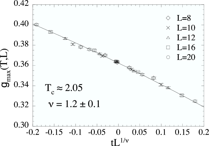
Figure 4: Scaling collapse of $g_{\rm max}(T,L)$ vs. $((T-T_{c})/T_{c})L^{1/\nu}$. The values of $T_{c}=2.051$ and $\nu=1.18$ from the last row of Table 1 are used. The solid curve is the fitted cubic polynomial.

Having found the value of $T_{c}$, we next determine the anisotropy exponent $\zeta$. In Fig. 5 we show a log-log plot of our data for $L_{z\,{\rm max}}$ vs. $L$, at the temperature $T=2.05\simeq T_{c}$. Fitting to Eq.(15), $L_{z\,{\rm max}}\sim L^{\zeta}$, we get the results summarized in Table 2 for different ranges of system sizes $L$. The results are consistent within the estimated statistical error and we find $\zeta=1.3\pm 0.1$. To check the consistency of our value for $\zeta$, in Fig. 6 we plot $g(T_{c},L,L_{z})$ vs. $L_{z}/L^{\zeta}$, using our data at $T=2.05$ and the above determined value of $\zeta=1.3$. As expected from Eq.(11), the data for the different values of $L$ and $L_{z}$ show a very good collapse to a single scaling curve.

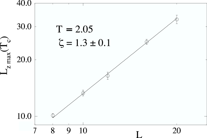
Figure 5: Log-log plot of $L_{z\,{\rm max}}$ vs. $L$, at $T=2.05\simeq T_{c}$. The solid straight line is the best power law fit using the data for $L=10-20$ and yields the value $\zeta=1.329\pm 0.08$ (see Table 2).

$L_{\rm min}$	$8$	$10$	$12$
$\zeta$	$1.29\pm 0.05$	$1.33\pm 0.08$	$1.37\pm 0.12$

Table 2: Anisotropy exponent $\zeta$ from power law fits, $L_{z\,{\rm max}}\sim L^{\zeta}$ to system sizes $L=L_{\rm min}-20$.

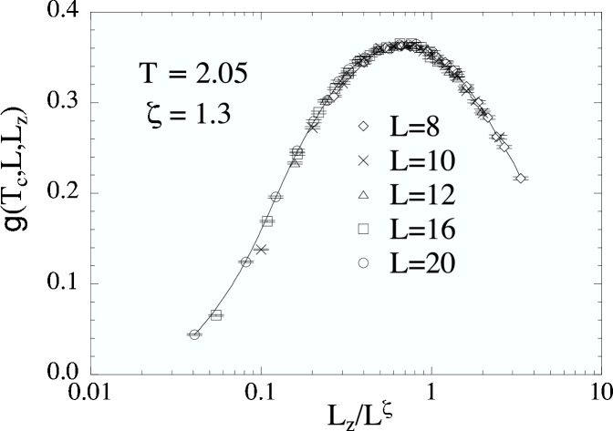
Figure 6: Scaling collapse of $g(T_{c},L,L_{z})$ vs. $L_{z}/L^{\zeta}$, for data at $T=2.05\simeq T_{c}$, using $\zeta=1.3$. The solid line is a guide to the eye only.

We have also tried a similar scaling analysis for the helicity moduli product, $L^{2}[\Upsilon_{x}\Upsilon_{z}]$, of Eq.(21). However here we have found less satisfactory results. We find that for a given system size $L$, the $L_{z\,{\rm max}}$ where $L^{2}[\Upsilon_{x}\Upsilon_{z}]$ has its maximum occurs at a smaller value of $L_{z}$ than was the case for the Binder ratio $g_{\rm max}$. Such smaller system sizes presumably have larger corrections to scaling. We have also found the statistical error in $L^{2}[\Upsilon_{x}\Upsilon_{z}]$ to be larger than we found for $g_{\rm max}$, possibly because the Binder ratio $g$ involves a ratio between fluctuating quantities and so has smaller sample to sample fluctuations.Huse As a consequence of these two effects, we could not arrive at a convincing determination of $T_{c}$ and $\nu$ from the $L^{2}[\Upsilon_{x}\Upsilon_{z}]$ data alone. However, to illustrate our results we can make use of the values of $T_{c}\simeq 2.05$ and $\zeta\simeq 1.3$ found in our analysis of $g_{\rm max}$. In Fig. 7 we therefore show a scaling collapse similar to that of Fig. 6, plotting $L^{2}[\Upsilon_{x}\Upsilon_{z}]$ vs. $L_{z}/L^{\zeta}$, using our data at $T=2.05\simeq T_{c}$ and the above value of $\zeta$.

We see clearly in Fig. 7 the above effects: error bars are considerably larger than in Fig. 6, and the peak is at a smaller value of $L_{z}/L^{\zeta}$. The scaling collapse is not bad for the bigger systems sizes, corresponding to larger values of $L_{z}/L^{\zeta}$. However it is rather scattered near the peak and below it. We conclude that it would be necessary to average over many more disorder realizations to reduce the errors, and perhaps also go to larger system sizes, in order to get a convincing scaling analysis from the helicity product $L^{2}[\Upsilon_{x}\Upsilon_{z}]$ on its own.

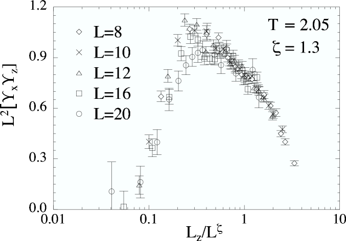
Figure 7: Attempted scaling collapse of $L^{2}[\Upsilon_{x}\Upsilon_{z}]$ vs. $L_{z}/L^{\zeta}$. Data is for $T=2.05\simeq T_{c}$, using $\zeta=1.3$.

IV Dynamic Critical Behavior

As one approaches the critical temperature $T_{c}$, we expect relaxation times to diverge as $\tau\sim\xi^{z}$, defining the dynamic critical exponent $z$. To compute equilibrium critical exponents, it is sufficient that the simulation dynamics satisfies detailed balance; the details of the dynamics are otherwise irrelevant. Thus the exact duality between ${\cal H}_{\rm XY}$ and ${\cal H}_{\rm loop}$ implies that the unscreened and the strongly screened superconductors have the same equilibrium critical behavior. For the dynamic critical behavior, however, the value of $z$ will in general depend on the details of the dynamics,Hohenberg and some works suggest that it may even vary for different types of relaxational dynamics or different boundary conditions.Minnhagen ; Minnhagen2 There is thus no reason, a priori, to expect the same dynamic critical behavior for the XY model, expressed in terms of a dynamical rule for the phase variables $\theta_{i}$, as compared to the loop model, expressed in terms of a dynamical rule for the vortex line variables $n_{i\mu}$. In this section, therefore, we will present results from explicit simulations of the loop model as well as the XY model.

Because the true dynamics of a superconductor is local, it is not physically meaningful to compute the dynamic critical exponent within accelerated global algorithms such as the Wolff algorithm, which we used to compute equilibrium properties. We therefore will use a local Monte Carlo dynamics for both ${\cal H}_{\rm XY}$ and ${\cal H}_{\rm loop}$. Even within such local algorithms, it is not obvious how universal the dynamical critical behaviors may be. Thus it is unclear that our results will correspond to what is seen in experiments. Nevertheless it will be interesting to see if the two models give similar or different values of $z$.

The relative loss of efficiency that results from using such local algorithms means that we will be unable to do as extensive an exploration of the parameter space as we did for our equilibrium analysis. But this is not necessary. We can make use of our already obtained equilibrium results, and simulate only at the value of $T=T_{c}$, using system aspect ratios $L_{z}=\gamma L^{\zeta}$. For our simulation of ${\cal H}_{\rm loop}$, we will simulate the loop model which is exactly dual (see Appendix A, Eq.(41)) to the cosine XY model that we have used in our equilibrium simulations, so as to make use of these known values of $T_{c}$ and $\zeta$.

IV.1 Monte Carlo Methods and Scaling

For the XY model of an unscreened superconductor we use a standard single spin heat bath algorithm, with fixed periodic boundary conditions on the $\theta_{i}$. In this algorithm, a phase angle $\theta_{i}$ is selected at random and replaced with a new randomly chosen $\theta_{i}^{\prime}$. This update attempt is then accepted with probability $1/[1+{\rm exp}(\Delta E/T)]$ where $\Delta E$ is the change in energy. One sweep, consisting of $N=L^{2}L_{z}$ update attempts, is taken as one time step, $\Delta t=1$. We average over $300-700$ disorder realizations depending on system size $L$.

For the loop model of a strongly screened superconductor, we again use a heat bath algorithm in which the attempted excitation consists of an elementary vortex loop circulating about a randomly chosen plaquette of the grid. Adding only such closed loop excitations corresponds to the ensemble in which the average internal magnetic field is constrained to ${\bf B}=0$ (see Appendix A). One sweep, consisting of $3N$ such update attempts, is taken as one time step, $\Delta t=1$. We average over $1000-2000$ disorder realizations depending on system size $L$.

In general, we expect the relaxation time $\tau$ to obey the scaling equation,

$$\tau(T,L,L_{z})=b^{z}\tilde{\tau}(tb^{1/\nu},L/b,L_{z}/b^{\zeta})\enspace,$$ (22)

where $b$ is an arbitrary length rescaling factor. For $b=L$, $T=T_{c}$, and $L_{z}=\gamma L^{\zeta}$, this reduces to the simple,

$$\tau\sim L^{z}\enspace.$$ (23)

For both the XY model and the loop model, we simulate with values of $L_{z}=\gamma L^{\zeta}$ as determined by the fit shown in Fig. 5. For the XY model, to approximate non-integer values of $L_{z}$ we use linear interpolation of simulation data for the two closest integer values of $L_{z}$. For the loop model we simply use results from the closest integer value of $L_{z}$.

IV.2 Observables

IV.2.1 XY Model

For the XY model we have tried two independent methods of determining $z$, analogous to the two quantities $g$ and $L^{2}[\Upsilon_{x}\Upsilon_{z}]$ used in our equilibrium simulations. The first is to look at the decay of correlations in the order parameter $M$ of Eq.(16), defining the relaxation time $\tau$ by,

$$\tau=1+2\sum_{t=1}^{t_{0}}\left[{\langle M(t)M(0)\rangle\over\langle M^{2}\rangle}\right]\sim L^{z}\enspace,$$ (24)

where $t_{0}$ is chosen large enough so that $\tau$ is independent of $t_{0}$. The ratio in the above ensures that the quantity being summed over has scaling dimension zero, and hence the sum scales as $\tau\sim L^{z}$.

The second method is to look at correlations of the supercurrent $I_{\mu}$, defined by,

$$I_{\mu}=\left.{\partial{\cal H}_{\rm XY}\over\partial\Delta_{\mu}}\right|_{\Delta_{\mu}=0}={1\over L_{\mu}}\sum_{i}J_{i\mu}\sin(\theta_{i+\hat{\mu}}-\theta_{i})\enspace.$$ (25)

In terms of $I_{\mu}$ one can define the conductance in the $\hat{\mu}$ direction by the Kubo formula,Minnhagen

$$G_{\mu}={1\over 2T}\sum_{t=-t_{0}}^{t_{0}}\Delta t\left[\langle I_{\mu}(t)I_{\mu}(0)\rangle\right]\sim L^{z}\enspace,$$ (26)

where again $t_{0}$ is chosen large enough that $G_{\mu}$ is independent of $t_{0}$. Since $I_{\mu}=\left.(\partial{\cal H}_{\rm XY}/\partial\Delta_{\mu})\right|_{\Delta_{\mu}=0}$, and ${\cal H}_{\rm XY}$ and $\Delta_{\mu}$ are scale invariant, then $I_{\mu}$, and hence the correlation summed over in in the definition of $G_{\mu}$, has scaling dimension zero. Therefore, the sum which defines $G_{\mu}$ scales as $\tau\sim L^{z}$.

IV.2.2 Loop Model

For the loop model we consider the total resistance, defined as follows.Wallin1 ; Wallin3 Let $Q_{\mu}(t)$ be the total projected loop area with normal in direction $\hat{\mu}$ at simulation time $t$. Each time an oriented elementary vortex loop with normal in direction $\pm\hat{\mu}$ is accepted, $Q_{\mu}$ changes by $\pm 1$. Let $\Delta Q_{\mu}(t)\equiv Q_{\mu}(t)-Q_{\mu}(t-1)$ be the total change in this area after one sweep through the entire system; each sweep represents $\Delta t=1$. In one such sweep, the total average phase angle change across the length of the system (in the dual screened XY superconductor model) in direction $\hat{\mu}$ is just $2\pi\Delta Q_{\mu}/L_{\nu}L_{\sigma}$, where $\mu$, $\nu$, $\sigma$ are a cyclic permutation of $x$, $y$, $z$. By the Josephson relation, the total voltage drop across the system in direction $\hat{\mu}$ will then be

$$V_{\mu}(t)=\left({\hbar\over 2e}\right)\left({2\pi\over L_{\nu}L_{\sigma}}\right)\left({\Delta Q_{\mu}\over\Delta t}\right)=\left({h\over 2e}\right)\left({1\over L_{\nu}L_{\sigma}}\right)\left({\Delta Q_{\mu}\over\Delta t}\right)\enspace.$$ (27)

Henceforth we define our units of voltage such that $h/2e\equiv 1$. We then define the total resistance in direction $\hat{\mu}$ by the Kubo formula,Young2

$$R_{\mu}={1\over 2T}\sum_{t=-t_{0}}^{t_{0}}\Delta t[\langle V_{\mu}(t)V_{\mu}(0)\rangle]\enspace,$$ (28)

where again $t_{0}$ is chosen large enough so that $R_{\mu}$ is independent of $t_{0}$. Since the total voltage drop $V_{\mu}$ is the time rate of change of the total phase angle difference across the system, and since the total phase angle difference is a scale invariant quantity, we have the scaling $V_{\mu}\sim 1/\tau$. Thus the resistance above scales as,

$$R_{\mu}\sim 1/\tau\sim L^{-z}\enspace.$$ (29)

IV.3 Results

IV.3.1 XY Model

In Fig. 8 we show a log-log plot of our results for the order parameter relaxation time $\tau$ of Eq.(24) vs. system size $L$, for $T=2.05\simeq T_{c}$ and $L_{z}\sim L^{\zeta}$. Our results are obtained using $5\times 10^{5}$ MC sweeps to equilibrate, followed by $10^{6}$ sweeps to compute averages. Fitting to the power law, $\tau\sim L^{z}$, we get the results summarized in Table 3, for different ranges of systems size $L$. The results are consistent within the estimated statistical error, with a small systematic tendency to lower values as we restrict the fitted data to larger system sizes. We find $z_{\rm XY}=2.63\pm 0.07$.

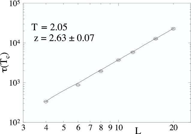
Figure 8: Log-log plot of order parameter relaxation time $\tau$ of Eq.(24) vs. system size $L$, for $T=2.05\simeq T_{c}$ and $L_{z}\sim L^{\zeta}$. Solid line is the best power law fit for sizes $L=10-20$, and determines $z=2.63\pm 0.07$ (see Table 3).

$L_{\rm min}$	$6$	$8$	$10$	$12$
$z_{\rm XY}$	$2.72\pm 0.04$	$2.69\pm 0.05$	$2.63\pm 0.07$	$2.60\pm 0.03$

Table 3: Dynamic exponent $z_{\rm XY}$ from power law fits, $\tau\sim L^{z}$, to system sizes $L=L_{\rm min}-20$.

As another check on our above determination of $z_{\rm XY}$, we consider the following. In principal, $\tau$ is defined by taking $t_{0}$ in Eq.(24) sufficiently large so that $\tau$ is independent of $t_{0}$; our data in Fig. 8 satisfies this condition. How big $t_{0}$ must be for this to happen is set by the time scale $\tau$ itself. Therefore, we expect that if we compute $\tau$ for arbitrary $t_{0}$, then $\tau(t_{0})$ should scale as,

$$\tau(t_{0})\sim L^{z}\tilde{\tau}(t_{0}/\tau)\sim L^{z}\tilde{\tau}(t_{0}/L^{z})\enspace.$$ (30)

In Fig. 9 we show a log-log plot of $\tau(t_{0})/L^{z}$ vs. $t_{0}/L^{z}$ for various sizes $L$ (again using $T=2.05\simeq T_{c}$ and $L_{z}\sim L^{\zeta}$). Choosing the value $z_{\rm XY}=2.63$ obtained from the fit in Fig. 8 we find an excellent collapse of all the data. For large $t_{0}/L^{z}$ we see that the curve does indeed saturate to a finite constant as expected, however the collapse holds for the entire range of $t_{0}$.

Figure 9: Log-log scaling plot of order parameter relaxation time $\tau(t_{0})/L^{z}$ vs. $t_{0}/L^{z}$ for $T=2.05\simeq T_{c}$, $L_{z}\sim L^{\zeta}$, and various values of $L$. Using $z_{\rm XY}=2.63$ gives an excellent collapse for the entire range of $t_{0}$.

Finally, we plot in Fig. 10 the conductances of Eq.(26), $G_{x}$ and $G_{z}$ vs. $L$, for $T=2.05\simeq T_{c}$ and $L_{z}\sim L^{\zeta}$. Our results are for $2\times 10^{5}$ MC sweeps to equilibrate, followed by $4\times 10^{5}$ sweeps to compute averages. Fitting to the power law, $G_{\mu}\sim L^{z_{\mu}}$, we get the results summarized in Table 4, for different ranges of systems size $L$. For $G_{x}$ the results $z\simeq 2.66\pm 0.04$ are consistent, within errors, with that obtained from our analysis of the order parameter relaxation time $\tau$. For $G_{z}$, we get values for $z$ that are somewhat larger. However if one compares the data points for $G_{x}$ and $G_{z}$ directly, one sees that the values are all roughly equal within the estimated error, except for the smallest size $L=4$ (probably too small to be in the scaling limit) and for the largest size $L=20$. Our fit for $z$ from the $G_{z}$ data is skewed by this one $L=20$ data point. If we restrict our fit to sizes $L=8-16$, we then find $z_{z}=2.82\pm 0.03$. This is still somewhat larger than what we get from $G_{x}$, but within two standard deviations of $z_{x}$ for the same range of sizes $L=8-16$.

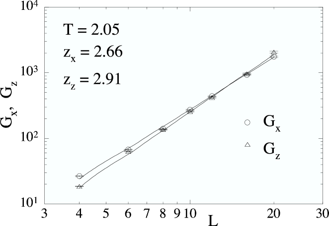
Figure 10: Log-log plot of conductances $G_{x}$ and $G_{z}$ vs. $L$, for $T=2.05\simeq T_{c}$ and $L_{z}\sim L^{\zeta}$. The fitted straight lines determine $z_{x}=2.66$ and $z_{z}=2.91$.

$L_{\rm min}$	$6$	$8$	$10$	$12$
$z_{x}$	$2.71\pm 0.02$	$2.75\pm 0.03$	$2.66\pm 0.04$	$2.69\pm 0.06$
$z_{z}$	$2.77\pm 0.02$	$2.87\pm 0.03$	$2.91\pm 0.04$	$3.06\pm 0.07$

Table 4: Dynamic exponent $z_{\rm XY}$ from power law fits, $G_{\mu}\sim L^{z_{\mu}}$, to system sizes $L=L_{\rm min}-20$.

IV.3.2 Loop Model

For our loop simulations we use the interaction of Eq.(41), exactly dual to our XY model. This interaction is computed using the same distribution of $J_{i\mu}$ as we used for the XY model, and we simulate at the same value of $T=2.05$ as gives the critical point of the XY model. We also use the same values of $L_{z}=\gamma L^{\zeta}$ as we used for the XY model, as determined from Fig. 5. In Fig. 11 we give our results for the resistance of the loop model, Eq.(28), as a log-log plot of $R_{x}$ and $R_{z}$ vs. system size $L$. Our results are from $12\times 10^{4}$ MC sweeps to equilibrate, followed by $24\times 10^{4}$ sweeps to compute averages. Fitting to the power law of Eq.(29), $R_{x}\sim L^{-z}$, we get the results summarized in Table 5, for different ranges of systems size $L$. The results are consistent within the estimated statistical error, and we find $z_{\rm loop}=3.4\pm 0.1$.

For the case of $R_{z}$, parallel to the columnar defects, our simulations were not sufficiently long to observe the necessary saturation of $R_{z}(t_{0})$ with increasing $t_{0}$, except for the smallest system sizes $L\leq 12$. We do not believe that any estimate of $z_{\rm loop}$ based on such small system sizes would be meaningful. We can, however, perform the following consistency check. Similar to our discussion concerning $\tau(t_{0})$ (see Eq.(30)), we can compute $R_{\mu}$ of Eq.(28) for finite times $t_{0}$, and we expect $R_{\mu}(t_{0})L^{z}$ to scale with the variable $t_{0}/L^{z}$. In Fig. 12 we make such a log-log scaling plot using the value of $z=3.4$ found for $R_{x}$ in Fig. 11. For $R_{x}$ we see that the collapse is excellent for all times $t_{0}$, and the scaling curve saturates to a constant at large $t_{0}/L^{z}$ as expected. For $R_{z}$, we find a good collapse for all but the largest times. We see that $R_{z}(t_{0})$ saturates only for the smallest systems, and it is only here that the collapse appears to be breaking down. We conclude that these small system sizes are not large enough to expect scaling for $R_{z}$ to hold.

We can also try to independently determine the dynamic exponent $z$ by fitting to a data collapse as in Fig. 12 for all times $t_{0}$, rather than just the asymptotic large time limit. The inset to Fig. 12 shows the resulting $\chi^{2}$ of such fits as the fitting parameter $z$ is varied. For $R_{x}$, the $\chi^{2}$ shows a sharp minimum at $z=3.45$, in good agreement with our earlier value of $z=3.4$ from Fig. 11. For $R_{z}$, the $\chi^{2}$ has a minimum at the somewhat higher value of $z=3.7$, however the minimum is very shallow, indicating a relative insensitivity of the data to variations in $z$. We conclude that both the data for $R_{x}$ and $R_{z}$ are consistent with a dynamic exponent $z_{\rm loop}=3.4\pm 0.1$.

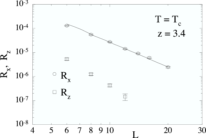
Figure 11: Log-log plot of resistance $R_{x}$ and $R_{z}$ of the loop model vs. $L$. The solid line is the best power law fit, $R_{x}\sim L^{-z}$, for sizes $L=10-20$, and determines the value $z_{\rm loop}=3.4\pm 0.1$ (see Table 5).

$L_{\rm min}$	$6$	$8$	$10$	$12$
$z_{\rm loop}$	$3.23\pm 0.05$	$3.33\pm 0.07$	$3.39\pm 0.11$	$3.38\pm 0.14$

Table 5: Dynamic exponent $z_{\rm loop}$ from power law fits, $R_{x}\sim L^{-z}$, to system sizes $L=L_{\rm min}-20$.

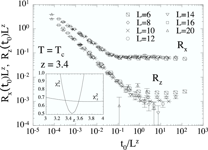
Figure 12: Log-log scaling plot of time dependent resistance $R_{x}(t_{0})L^{z}$ and $R_{z}(t_{0})L^{z}$ of the loop model vs. $t_{0}/L^{z}$. The value $z=3.4$ obtained from the fit in Fig. 11 is used. The inset gives the $\chi^{2}$ error of the data collapse, as the exponent $z$ is varied.

V Discussion and Conclusions

We have studied the equilibrium and dynamic critical behavior of the zero magnetic field superconducting phase transition for a type-II superconductor with quenched columnar disorder. We have considered both the “unscreened” XY model in which $\lambda_{0}\to\infty$, and the “strongly screened” loop model in which $\lambda_{0}\sim\xi_{0}$. A duality transformation establishes that these two models are in the same equilibrium universality class. Using numerical simulations of the XY model, we find, in agreement with a generalized Harris criterion, that the universality class of the transition is different from the pure model, and we find that scaling is anisotropic. We find the value for the correlation length exponent, $\nu=1.2\pm 0.1$, and for the anisotropy exponent, $\zeta=1.3\pm 0.1$.

Using the value of the critical temperature and the anisotropic scaling determined from the equilibrium analysis, we carry out simulations at the critical point to determine the dynamic critical exponent $z$ of both the XY and loop models for local Monte Carlo dynamic rules. For the “unscreened” XY model, with a single spin heat bath dynamics, we find $z_{\rm XY}=2.6\pm 0.1$. For the “strongly screened” loop model, with a heat bath dynamics applied to elementary loop excitations, we find $z_{\rm loop}=3.4\pm 0.1$.

A similar random 3D XY model has been studied by Cha and GirvinCha in the context of the quantum phase transition in the two dimensional boson Hubbard model. In their model disorder was introduced as uniformly distributed random bonds in the $\hat{z}$ (imaginary time) direction, $J_{iz}$, so as to model bosons with random charging energy. They found equilibrium critical exponents $\nu=1.0\pm 0.3$ and $\zeta=1.07\pm 0.03$ (our anisotropy exponent $\zeta$ for the classical 3D model is equivalent to their “quantum dynamic exponent” $z$ for the 2D quantum problem). However their analysis for such a system with anisotropic scaling, $\zeta>1$, was based on a more ad hoc approach of (i) trying various values of $\zeta$ and seeing which appeared to give the best data collapse for systems of different size $L$, and (ii) measuring real space correlations in a system of a fixed size and fitting to assumed power law decays. Their largest system size, $16^{2}\times 15$ is also smaller than ours and they do not use the Wolff algorithm to accelerate their equilibration. While it is possible that introducing the randomness differently (along $\hat{z}$ rather than in the $xy$ plane) might effect the universality class, we believe it is more likely that this is not the case, and that our results are more systematic and hence more accurate than those of Cha and Girvin.

Prokof’ev and SvistunovSvistunov have simulated the loop model of Eq.(5) in the context of the same two dimensional disordered boson problem as Cha and Girvin. For their “off-diagonal” disorder case they put the disorder into the bonds along the $\hat{z}$ direction, making their model dual to that of Cha and Girvin. They report an anisotropy exponent $\zeta=1.5\pm 0.2$, which agrees with ours within the estimated errors. They were unable to determine the correlation length exponent $\nu$. We note that while they use an accelerated “worm” algorithm and have good statistics for quite large system sizes, they determine their exponents by fitting to real space correlation functions for their biggest size system, as did Cha and Girvin, rather than doing any systematic finite size scaling that takes into account the anisotropic scaling present in the model.

Experimental investigation of the zero field transition with colummnar disorder has been undertaken by Kötzler and co-workersKotzler for YBaCuO thin films. Measuring the frequency dependent conductivity transverse to the columnar disorder, which is expected to scale asFisher $\sigma_{\perp}(\omega,T)=t^{(\zeta-z)\nu}\tilde{\sigma}(\omega t^{-z\nu})$ (where $t=(T-T_{c})/T_{c}$), they findnote the combinations $\nu\zeta=1.7$ and $z/\zeta=5.53$. This compares with our values $\nu\zeta=1.56$, and $z/\zeta=2$ for the unscreened XY model, and $z/\zeta=2.6$ for the strongly screened loop model. Our value of $\nu\zeta$ is conceivably consistent with the experimental value, within possible errors. However both of our values of $z/\zeta$ seem too small. It may be that our simple local Monte Carlo dynamics does not adequately capture the true dynamics of a real superconductor. On the other hand, if we use our value of $\zeta=1.3$, then Kötzler’s results imply a dynamic exponent of $z=7.2$, which seems extraordinarily large.

We may also compare our dynamic exponents with those obtained from the disorder free model. For the the strongly screened limit of the loop model, Lidmar et al.Wallin4 find the value $z_{\rm loop}\simeq 2.7$; moreover they find this value to be insensitive to the presence of uncorrelated point disorder. For relaxational dynamics of the phase angle variable in the XY model, a value of $z\approx 2$ is expected,Hohenberg and this is what was found in numerical simulations by Jensen et al.Minnhagen using a method similar to our scaling of conductance, Eq.(26). The result $z_{\rm loop}>z_{\rm XY}$ thus seems common for both the pure and columnar disordered cases.

In our work we have considered only simple relaxational dynamics for the phase angles of the unscreened XY model. Two other possible dynamics might be considered. One would be to do a loop dynamics, similar to what we have done here for the strongly screened loop model, only now as applied to the strongly interacting loops of the unscreened XY model. The other would be to use resistively shunted junction (RSJ) dynamics for the phase angles of the XY model. Both such approaches have been previously used for the disorder free case. For both loop dynamicsWallin4 ; Weber and RSJ dynamicsMinnhagen ; Stroud the dynamic exponent $z\simeq 1.5$ was found, smaller than the value obtained by simple phase angle relaxational dynamics. Investigating these other dynamics for the case of columnar disorder remains for future work. We only note here that if the above trend remains true for columnar disorder, and that these other dynamics reduce $z$ from that of relaxational dynamics, then it becomes even harder to explain the large value of $z\zeta$ observed experimentally in Ref. Kotzler, .

Finally, we note that similar equilibrium exponents to those found in this work were also found for the case of an unscreened superconductor with columnar defects in a finite applied magnetic field. For that case the valuesWallin2 $\nu=1.0\pm 0.1$ and $\zeta=1.25\pm 0.1$ were found. Although these are close to the values we find here for zero applied field, there is no apparent reason that the zero and finite field cases should be in the same universality class. We also note that once a finite field is applied, the duality between the unscreened and strongly screened superconductor models, that exists for zero field, breaks down.

Appendix A

In this section we review the duality transformationDasgupta ; Kleinert ; Savit from ${\cal H}_{\rm XY}$ of Eq.(1) to ${\cal H}_{\rm loop}$ of Eq.(5). Consider first a general $2\pi$ periodic interaction $V_{i\mu}(\phi)$ instead of the $-(J_{i\mu}/T)\cos(\phi)$ of Eq.(1). For the generalized fixed twist boundary condition and the corresponding Hamiltonian of Eq.(4), we can write the partition function as,

$$Z=\left(\prod_{i}\int_{0}^{2\pi}{d\theta^{\prime}_{i}\over 2\pi}\right){\rm e}^{-\sum_{j\mu}V_{j\mu}(\theta^{\prime}_{j}-\theta^{\prime}_{j+\hat{\mu}}-\Delta_{\mu}/L_{\mu})}\enspace.$$ (31)

where the $\theta^{\prime}_{i}$ obey periodic boundary conditions. Defining the Fourier transform $\tilde{V}_{j\mu}$ by,

$${\rm e}^{-V_{j\mu}(\phi)}\equiv\sum_{n_{j\mu}=-\infty}^{\infty}{\rm e}^{-\tilde{V}_{j\mu}(n_{j\mu})}{\rm e}^{in_{j\mu}\phi}\enspace,$$ (32)

and substituting into Eq.(31) gives,

$$Z = \sum_{\{n_{j\mu}\}}\left(\prod_{i}\int_{0}^{2\pi}{d\theta^{\prime}_{i}\over 2\pi}\right){\rm e}^{-\sum_{j\mu}\tilde{V}_{j\mu}(n_{j\mu})+i\sum_{j\mu}n_{j\mu}(\theta^{\prime}_{j}-\theta^{\prime}_{j+\hat{\mu}}-\Delta_{\mu}/L_{\mu})}$$ (33)

$$= \sum_{\{n_{j\mu}\}}{\rm e}^{-\sum_{j\mu}\left[\tilde{V}_{j\mu}(n_{j\mu})+in_{j\mu}\Delta_{\mu}/L_{\mu}\right]}\left(\prod_{i}\int_{0}^{2\pi}{d\theta^{\prime}_{i}\over 2\pi}\right){\rm e}^{i\sum_{j\mu}n_{j\mu}(\theta^{\prime}_{j}-\theta^{\prime}_{j+\hat{\mu}})}\enspace.$$ (34)

One is now free to do the integrals over the $\theta^{\prime}_{j}$. The result is a product of Kronecker deltas constraining the variables $n_{j\mu}$ to be divergenceless, as in Eq.(6). Defining the “winding numbers” $W_{\mu}$ by,

$$W_{\mu}\equiv{1\over L_{\mu}}\sum_{i}n_{i\mu}\enspace,$$ (35)

we get,

$$Z={\sum_{\{n_{j\mu}\}}}^{\prime}{\rm e}^{-\sum_{j\mu}\tilde{V}_{j\mu}(n_{j\mu})-i\sum_{\mu}W_{\mu}\Delta_{\mu}}\enspace,$$ (36)

where the prime on the summation denotes the divergenceless constraint of Eq.(6).

A common choice for $V_{i\mu}(\phi)$ is the Villain interaction,Villain

$${\rm e}^{-V_{j\mu}(\phi)}\equiv\sum_{m=-\infty}^{\infty}{\rm e}^{-{J_{j\mu}\over 2T}(\phi-2\pi m)^{2}}\enspace.$$ (37)

In this case one has for its transform,

$$\tilde{V}_{i\mu}(n)={T\over 2J_{i\mu}}n^{2}\enspace.$$ (38)

The partition function of Eq,(36), with periodic boundary conditions $\Delta_{\mu}=0$, then becomes,

$$Z={\sum_{\{n_{j\mu}\}}}^{\prime}{\rm e}^{-{1\over 2\tilde{T}}\sum_{j\mu}g_{j\mu}n_{j\mu}^{2}}\enspace,$$ (39)

with

$$g_{i\mu}/\tilde{T}=T/J_{i\mu}\enspace.$$ (40)

The above is just a model of short ranged interacting loops with onsite repulsion $\sim n^{2}$ and inverted temperature scale $\tilde{T}\sim 1/T$.

For our simulatons, with $V_{i\mu}(\phi)=-(J_{i\mu}/T)\cos(\phi)$, one hasSavit

$${\rm e}^{-\tilde{V}_{i\mu}(n)}=I_{n}(J_{i\mu}/T)\enspace,$$ (41)

where $I_{n}(x)$ is the modified Bessel function of the first kind. Since $I_{n}(x)$ is an increasing function of $|n|$ for fixed $x$, the above similarly gives a short ranged loop model with onsite repulsion. It is this interaction of Eq.(41) that we use in our dynamic simulations of the loop model in Section IV.

We can now demonstrate several interesting results concerning phase coherence in the XY model, by considering the behavior as a function of the twist $\Delta_{\mu}$. The XY model is phase coherent when the total free energy ${\cal F}$ varies with $\Delta_{\mu}$. Using ${\cal F}(\Delta_{\mu})=-T\ln Z(\Delta_{\mu})$, and Eq.(36) above, we find,

$${1\over T}\left.{\partial{\cal F}\over\partial\Delta_{\mu}}\right|_{\Delta_{\mu}=0}=i\langle W_{\mu}\rangle_{0}\enspace,$$ (42)

where $\langle\dots\rangle_{0}$ indicates an average in the ensemble with $\Delta_{\mu}=0$. Now since $\partial{\cal F}/\partial\Delta_{\mu}$ must be a real quantity (as may be seen by considering its evaluation in the original XY model ${\cal H}_{\rm XY}$ of Eq.(4)), and since $\langle W_{\mu}\rangle_{0}$ must similarly be real (as may be seen by considering ${\cal H}_{\rm loop}$), the only way for Eq.(42) to hold is if $\left.\partial{\cal F}/\partial\Delta_{\mu}\right|_{\Delta_{\mu}=0}=\langle W_{\mu}\rangle_{0}=0$. This then demonstrates that $\Delta_{\mu}=0$, i.e. periodic boundary conditions on the $\theta_{i}$, is the twist that minimizes the free energy.

Finally, returning to Eq.(36), we note that in the fluctuating twist ensembleOlsson for the XY model, in which $\Delta_{\mu}$ is averaged over as a thermally fluctuating degree of freedom, the corresponding loop model obeys the additional constraint of zero winding, $W_{\mu}=0$, in each individual configuration. When viewing ${\cal H}_{\rm loop}$ as the Hamiltonian of vortex loops in a strongly screened superconductor, this corresponds to the ensemble in which the average internal magnetic field is constrained to vanish, $B_{\mu}=0$, in each configuration.

References

- (1) For reviews see, G. Blatter, M. V. Feigel’man, V. B. Geshkenbein, A. I. Larkin and V. M. Vinokur, Rev. Mod. Phys. 66, 1125 (1994); E. H. Brandt, Rep. Prog. Phys. 58, 1465 (1995); T. Nattermann and S. Scheidl, Adv. Phys. 49, 607 (2000).
- (2) D. R. Nelson and V. M. Vinokur, Phys. Rev. Lett. 68, 2398 (1992); Phys. Rev. B48, 13060 (1993); ibid 61, 5917 (2000).
- (3) J. Lidmar and M. Wallin, Europhys. Lett. 47, 494 (1999).
- (4) A. Vestergren, J. Lidmar and M. Wallin, Phys. Rev. B 67, 92501 (2003).
- (5) M. Wallin, E. S. Sørenson, S. M. Girvin and A. P. Young, Phys. Rev. B 49, 12115 (1994).
- (6) J. T. Chayes, L. Chayes, D. S. Fisher and T. Spencer, Phys. Rev. Lett. 57, 2999 (1986); Commun. Math. Phys. 120 501 (1989).
- (7) A. B. Harris, J. Phys. C 7, 1671 (1974).
- (8) C. Dasgupta and B. I. Halperin, Phys. Rev. Lett. 47, 1556 (1981).
- (9) M.-C. Cha and S. M. Girvin, Phys. Rev. B49, 9749 (1994).
- (10) N. Prokof’ev and B. Svistunov, Phys. Rev. Lett. 92, 15703 (2004).
- (11) D. Jaksch, C. Bruder, J. I. Cirac, C. W. Gardiner and P. Zoller, Phys. Rev. Lett. 81, 3108 (1998); B. Damski, J. Zakrzewski, L. Santos, P. Zoller and M. Lewenstein, Phys. Rev. Lett. 91, 080403 (2003).
- (12) S. Sachdev, Quantum Phase Transitions, (Cambridge, 1999).
- (13) Y.-H. Li and S. Teitel, Phys. Rev. Lett. 66, 3301 (1991); Phys. Rev. B 47, 359 (1993); T. Chen and S. Teitel, Phys. Rev. B 55, 15197 (1997).
- (14) D. S. Fisher, M. P. A. Fisher and D. A. Huse, Phys. Rev. B 43, 130 (1991).
- (15) J. Lidmar, M. Wallin, C. Wengel, S. M. Girvin and A. P. Young, Phys. Rev. B 58, 2827 (1998).
- (16) H. Kleinert, Gauge Fields in Condensed Matter, (World Scientific, Singapore, 1989), Vol. 1; T. Banks, R. J. Myerson and J. Kogut, Nucl. Phys. B 129, 493 (1977).
- (17) R. Savit, Phys. Rev. B 17, 1340 (1978).
- (18) J. Villain, J. Phys. Paris 36, 581 (1975).
- (19) H. Rieger and A. P. Young, Phys. Rev. Lett. 72, 4141 (1994); M. Guo, R. N. Bhatt and D. A. Huse, Phys. Rev. Lett. 72, 4137 (1994).
- (20) M. P. Nightingale and H. W. Blöte, Phys. Rev. Lett. 60, 1562 (1988).
- (21) K. Binder, Phys. Rev. Lett. 47, 693 (1981).
- (22) T. Olson and A. P. Young, Phys. Rev. B61, 12467 (2000).
- (23) J. D. Reger, T. A. Tokuyasu, A. P. Young and M. P. A. Fisher, Phys. Rev. B 44, 7147 (1991).
- (24) U. Wolff, Phys. Rev. Lett. 62, 361 (1989).
- (25) D. A. Huse, private communication.
- (26) P. C. Hohenberg and B. I. Halperin, Rev. Mod. Phys. 49, 435 (1977).
- (27) L. M. Jensen, B. J. Kim and P. Minnhagen, Phys. Rev. B 61, 15412 (2000) and Europhys. Lett. 49, 644 (2000).
- (28) P. Minnhagen, B. J. Kim and H. Weber, Phys. Rev. Lett. 87, 37002 (2001).
- (29) A. P. Young, in Random Magnetism, High-Temperature Superconductivity”, eds. W. P. Beyerman, N. L. Huang-Liu and D. E. MacLaughlin (World Scientific, Singapore, 1994).
- (30) G. Nakielski, A. Rickertsen, T. Steinborn, J. Wiesner, G. Wirth, A. G. M. Jansen and J. Kötzler, Phys. Rev. Lett. 76, 2567 (1996); J. Kötzler, in Advances in Solid State Physics 39, ed. B. Kramer, (F. Vieweg & Sohn Verlags-GmbH, Braunschweig/Wiesbaden, 1999), p. 371 (also as cond-mat/9904279).
- (31) Due to differences of notation, the exponents and in Ref. Kotzler, correspond to our , and .
- (32) H. Weber and H. J. Jensen, Phys. Rev. Lett. 78, 2620 (1997).
- (33) K. H. Lee and D. Stroud, Phys. Rev. B 46, 5699 (1992).
- (34) P. Olsson, Phys. Rev. Lett. 73, 3339 (1994) and Phys. Rev. B 52, 4511 (1995).