A Generalized Epidemic Process and Tricritical Dynamic Percolation

Abstract

The renowned general epidemic process describes the stochastic evolution of a population of individuals which are either susceptible, infected or dead. A second order phase transition belonging to the universality class of dynamic isotropic percolation lies between endemic or pandemic behavior of the process. We generalize the general epidemic process by introducing a fourth kind of individuals, viz. individuals which are weakened by the process but not yet infected. This sensibilization gives rise to a mechanism that introduces a global instability in the spreading of the process and therefore opens the possibility of a discontinuous transition in addition to the usual continuous percolation transition. The tricritical point separating the lines of first and second order transitions constitutes a new universality class, namely the universality class of tricritical dynamic isotropic percolation. Using renormalized field theory we work out a detailed scaling description of this universality class. We calculate the scaling exponents in an $\varepsilon$-expansion below the upper critical dimension $d_{c}=5$ for various observables describing tricritical percolation clusters and their spreading properties. In a remarkable contrast to the usual percolation transition, the exponents $\beta$ and ${\beta}^{\prime}$ governing the two order parameters, viz. the mean density and the percolation probability, turn out to be different at the tricritical point. In addition to the scaling exponents we calculate for all our static and dynamic observables logarithmic corrections to the mean-field scaling behavior at $d_{c}=5$.

I Introduction

The formation and the properties of random structures have been a major theme in statistical physics for many years. In case the formation of such structures obeys local rules, these processes can often be expressed in the language of population growth. It is well known that two particular growth processes lead to random structures with the properties of percolation clusters. The so called simple epidemic process (SEP) leads to directed percolation (DP) BrHa57 ; CaSu80 ; Ob80 ; Hin00 . The SEP is also known as epidemic with recovery, Gribov process GraSu78 ; GraTo79 , as the stochastic version of Schlögls first reaction Ja81 ; Schl72 or in elementary particle physics as Reggeon field theory Gri67 ; GriMi68 ; Mo78 . The so called general epidemic process (GEP) Mol77 ; Bai75 ; Mur89 , also known as epidemic with removal, generates isotropic percolation (IP) clusters Gra83 ; Ja85 ; CaGra85 ; StAh92BuHa96 and models therefore the universality class of dynamic isotropic percolation (dIP).

Epidemic models like the SEP and the GEP are relevant for a wide range of systems in physics, chemistry, biology, and sociology. Undoubtedly, the potential of such simple models has its limitations because they rely on strong simplifying assumptions such as the homogeneity of the substrate footnote_quenchedDisorder , isotropy of the infections, immobility of individuals and so on. However, the transition between population survival and extinction of these processes is a nonequilibrium continuous (second order) phase transition phenomenon and hence is characterized by universal scaling laws which are shared by entire classes of systems. Near these transitions, simplistic epidemic models like the SEP and the GEP are of great value, because they are powerful workhorses to study the mutual properties of their entire universality class which also should include more realistic models.

The universal properties of DP and dIP are well known today thanks to numerous studies of the SEP and GEP, respectively. Relatively little is known, on the other hand, whether and under what modifications these stochastic growth processes allow for first order phase transitions between their endemic and pandemic states, and by the same token, for tricritical behavior at the phase-space boundary between first and second order transition. In the context of DP, these questions where addressed to some extend by Ohtsuki and Keyes OhKe87 . In this paper we will study this intriguing topic in the context of dIP by generalizing the famous GEP.

The standard GEP, assumed for simplicity to take place on a lattice Gra83 , can be described with help of the reaction scheme

$$S(\mathbf{n})+X(\mathbf{m})\quad \overset{\kappa}{\longrightarrow}\quad X(\mathbf{n})+X(\mathbf{m})\,,$$ (1a)

$$X(\mathbf{n})\quad \overset{\lambda}{\longrightarrow}\quad E(\mathbf{n})\,,$$ (1b)

with reaction rates $$\kappa \lambda S X E \mathbf{n} \mathbf{m} \kappa \lambda \kappa/\lambda \lambda \kappa=\kappa_{c} \kappa>\kappa_{c} P(\kappa) \kappa \kappa_{c}$$ and . , , and respectively denote susceptible, ill, and dead (or immune) individuals on nearest neighbor sites and . A susceptible individual may be infected by an ill neighbor with probability [reaction (1a)]. By this mechanism the disease (henceforth also called the agent) spreads diffusively. Ill individuals die with a probability [reaction (1b)]. There is no healing of infected individuals and no spontaneous infection. In a finite system the manifold of states without any infected individual is inevitably absorbing. Whether a single infected site leads to an everlasting epidemic in an infinite system depends on the ratio . With fixed there is a certain value that for all an eternal epidemic (a pandemic) occurs. The probability for the occurrence of a pandemic as a function of goes to zero continuously at the critical point . The behavior of the model near this critical point is in the universality class of dIP.

Of course, one can conceive many alterations of the GEP. Some modifications will lead to models which still belong to the dIP universality class whereas other alterations will produce models belonging to other universality classes. As an example for the latter, one might think of mobile susceptible or immune individuals which, say, diffuse through space. The resulting models are reaction-diffusion type models which have nothing to do with dIP footnote_diff_sick . We are not interested in this kind of alterations. Rather, we are interested in modifications of the GEP that preserve the dIP universality class and which, for certain parameter values, allow for tricriticality and first order percolation transitions. To be more specific, we are interested in the most relevant mechanism leading to tricritical and first order dIP. In spirit our model is closely related to the canonical model for tricriticality in eqilibrium systems, viz. the $\phi^{4}$ model with an additional $\phi^{6}$ term where the free energy density is of the form $f=\tau\phi^{2}+g_{4}\phi^{4}+g_{6}\phi^{6}$  tomsBook . If $g_{4}$ is positive then higher order terms including the $\phi^{6}$ term are irrelevant and one has in mean field theory a second order transition when $\tau$ passes through zero. Otherwise, however, one has an instability and higher order terms are required for stabilization of which the $\phi^{6}$ term is the most relevant one. For $g_{4}<0$ one has a first order transition at a critical value of $\tau$ that depends on $g_{4}$ and $g_{6}$ and the point $\tau=g_{4}=0$ constitutes a tricritical point. Our model to be defined in the next paragraph is so that it introduces a similar instability in the GEP and via this instability it allows for tricriticality and first order percolation. In its field theoretic description our model features, compared to the standard GEP, an additional higher order term which becomes the most relevant stabilizing term when the usual GEP coupling vanishes.

Our modification of the GEP can be defined in simple terms. The basic idea is to enrich the reaction scheme (1) by introducing weak individuals $Y$. Instead of being infected right away by an ill neighbor, any susceptible individual may be weakened with a reaction rate $\mu$ by such an encounter. When the disease passes by anew, a weakened individual is more sensitive and gets sick with a rate $\nu>\kappa$. In the following we refer to this model as the generalized GEP (GGEP). In addition to the reactions (1), the GGEP is described by the reactions

$$S(\mathbf{n})+X(\mathbf{m})\quad \overset{\mu}{\longrightarrow}\quad Y(\mathbf{n})+X(\mathbf{m})\,,$$ (2a)

$$Y(\mathbf{n})+X(\mathbf{m})\quad \overset{\nu}{\longrightarrow}\quad X(\mathbf{n})+X(\mathbf{m})\,.$$ (2b)

As we go along, we will show that the occurrence of the weak individuals gives rise to an instability that can lead to a discontinuous transition and compact (Eden Ed81 ; Ca83 ) growth of the epidemic if $$\nu \nu_{c}(\kappa,\mu) \kappa \mu \nu \lambda P(\kappa,\mu,\nu)$$ is greater than a critical value . In the enlarged three-dimensional phase space spanned by , , and with fixed , there exists a critical surface associated with the usual continuous percolation transition and a surface of first order transitions characterized by a finite jump in the probability for the occurrence of a pandemic. These two surfaces of phase transitions meet at a line of tricritical points.

The focus of this paper lies on the universal properties of the GGEP near this tricritical line. By using the methods of renormalized field theory we work out a scaling description of the new universality class of tricritical dynamic isotropic percolation (TdIP) to which the tricritical GGEP belongs. We study a multitude of static and dynamic observables that play important roles in percolation theory. In particular we calculate the critical exponents describing the scaling behavior of these observables below 5 dimensions as well as logarithmic corrections to the mean-field scaling behavior in 5 dimensions.

The outline of our paper is as follows. In Sec. II we consider the GGEP in a mean-field theory. As the main result of Sec. II, the mean-field analysis will reveal the structure of the phase diagram. With the aim of studying the effects of fluctuations, we condense the principles defining TdIP into a field theoretic model in Sec. III. In Sec. IV we work out the scaling properties of static aspects of TdIP. Section V treats the dynamic scaling properties. Concluding remarks are provided in Sec. VI. There is one Appendix in which we sketch the calculation of a parameter integral that is helpful in computing Feynman diagrams.

II Mean-Field Theory

A mean-field description of the GGEP can be formulated by treating the reaction equations (1) and (2) as deterministic equations without fluctuations. This deterministic approximation leads to the system of differential equations

$$\dot{S}(\mathbf{n},t) =-(\kappa+\mu)S(\mathbf{n},t)\sum_{\mathbf{m}}^{nn(\mathbf{n})}X(\mathbf{m},t)\,,$$ (3a)

$$\dot{Y}(\mathbf{n},t) =\Big{(}\mu S(\mathbf{n},t)-\nu Y(\mathbf{n},t)\Big{)}\sum_{\mathbf{m}}^{nn(\mathbf{n})}X(\mathbf{m},t)\,,$$ (3b)

$$\dot{X}(\mathbf{n},t) =\Big{(}\kappa S(\mathbf{n},t)+\nu Y(\mathbf{n},t)\Big{)}\sum_{\mathbf{m}}^{nn(\mathbf{n})}X(\mathbf{m},t)$$

$$-\lambda X(\mathbf{n},t)\,,$$ (3c)

$$\dot{E}(\mathbf{n},t) =\lambda X(\mathbf{n},t)$$ (3d)

governing the dynamics of the different kinds of individuals. Here, $$\sum_{\mathbf{m}}^{nn(\mathbf{n})} \mathbf{n}$$ denotes summation over the nearest neighbors of . At each lattice site there is the additional constraint

$$S+X+Y+E=1\,.$$ (4)

Thus, $S$, $X$, $Y$, and $E$ can be interpreted as the probability of finding the corresponding state at a site $\mathbf{n}$. Note that the processes can only proceed at places where the probability to find ill individuals in the neighborhood is not zero. We use the canonical initial condition that all sites of the initial state are susceptible except for the site at the origin which is ill, $X_{0}(\mathbf{n})=\delta_{\mathbf{n},0}$ and $Y_{0}(\mathbf{n})=E_{0}(\mathbf{n})\equiv 0$.

Equations (3a) and (3b) are are readily integrated. We obtain

$$S(\mathbf{n},t)=S_{0}(\mathbf{n})\exp\bigg{(}-\rho\sum_{\mathbf{m}}^{nn(\mathbf{n})}E(\mathbf{m},t)\bigg{)}$$ (5)

and

$$\mu S(\mathbf{n},t)+(\rho-\nu)Y(\mathbf{n},t) =\Big{(}\mu S_{0}(\mathbf{n})+(\rho-\nu)Y_{0}(\mathbf{n})\Big{)}$$

$$\times\exp\bigg{(}-\nu\sum_{\mathbf{m}}^{nn(\mathbf{n})}E(\mathbf{m},t)\bigg{)}\,,$$ (6)

where we have defined $\rho=\kappa+\mu$. The time scale $\lambda$ has been set to unity for simplicity. Equation (3d) together with the constraint (4) leads finally to the mean-field equation of motion of the GGEP,

$$\dot{E}(\mathbf{n},t) =1-E(\mathbf{n},t)$$

$$-\bigg{\{}\frac{\rho-\kappa}{\rho-\nu}\,\exp\bigg{(}-\nu\sum_{\mathbf{m}}^{nn(\mathbf{n})}E(\mathbf{m},t)\bigg{)}$$

$$+\frac{\kappa-\nu}{\rho-\nu}\exp\bigg{(}-\rho\sum_{\mathbf{m}}^{nn(\mathbf{n})}E(\mathbf{m},t)\bigg{)}\bigg{\}}\,S_{0}(\mathbf{n})\,.$$ (7)

In the asymptotic regime $|\mathbf{n}|,t\rightarrow\infty$ one can neglect time and space dependence in (7) and use the approximation $\sum_{\mathbf{m}}^{nn(\mathbf{n})}E(\mathbf{m},t)\approx zE(\mathbf{n},t)$, $z$ being the coordination number of the lattice. Hence the asymptotic values of $E$ are the solutions of the equation of state

$$E=\frac{\rho-\kappa}{\rho-\nu}\left(1-\mathrm{e}^{-z\nu E}\right)+\frac{\kappa-\nu}{\rho-\nu}\left(1-\mathrm{e}^{-z\rho E}\right)=:f(E)\,.$$ (8)

By setting $\rho=\kappa$, corresponding to $\mu=0$, one obtains the equation of state of the usual GEP Gra83

$$E=1-\mathrm{e}^{-z\kappa E}$$ (9)

with $\kappa=\kappa_{c}=1/z$ determining the second order phase transition corresponding to ordinary isotropic percolation. For $\kappa<\kappa_{c}$, Eq. (9) has only the solution $E=0$ which means that the disease does not percolate, i.e., is endemic. In the other case, $\kappa>\kappa_{c}$, a stable solution $E>0$ arises, signalling the percolative pandemic character of the disease. These types of solutions exist also in the full equation of state (8). Using $\kappa\leq\rho$, one demonstrates easily that $f(E)$ increases monotonically from zero to one in the interval $0\leq E<\infty$. Thus, $E=0$ is always a solution of Eq. (8). It follows from the equation of motion (7) that only solutions of Eq. (8) with $f^{\prime}(E)<1$ are stable. Because $f^{\prime}(0)=z\kappa$, a stable percolating solution $E>0$ exists always for $\kappa>\kappa_{c}$. The existence of more than one nontrivial solution requires necessarily that $f^{\prime\prime}(E)=0$ at least for one value $E>0$. From Eq. (8) we derive the inequality

$$f^{\prime\prime}(E)/z^{2}\leq\Big{(}\rho\nu-\kappa(\rho+\nu)\Big{)}\exp(-zE\max(\rho,\nu))\,.$$ (10)

With $f^{\prime\prime}(E)<0$ for $E\gg 1$ and $f^{\prime\prime}(0)/z^{2}=\rho\nu-\kappa(\rho+\nu)$ we therefore find

$$\frac{1}{\kappa}>\frac{1}{\rho}+\frac{1}{\nu}\ ,\quad\kappa<\kappa_{c}$$ (11)

as the necessary and sufficient conditions for the existence of a second locally stable solution $E>0$ besides $E=0$ with a discontinuous transition between the two. The line of tricritical points where the first and the second order transitions meet in the $\kappa$-$\rho$-$\nu$ phase space is determined by $1/\kappa=1/\rho+1/\nu=z$.

In the following we focus on the phenomena arising near the tricritical line. In this region of the phase space, $E(\mathbf{n,}t)$ is, except for a microscopic region around the origin $\mathbf{n}=\mathbf{0}$ of the position space, small and slowly varying. Hence, we may approximate Eq. (7) by the deterministic reaction-diffusion equation

$$\dot{E}(\mathbf{x},t) =D\nabla^{2}E(\mathbf{x},t)-\lambda\bigg{[}\tau E(\mathbf{x},t)$$

$$+\frac{f}{2}E(\mathbf{x},t)^{2}+\frac{g}{6}E(\mathbf{x},t)^{3}\bigg{]},$$ (12)

where $D=\kappa a^{2}$, with $a$ being the lattice constant, $\tau=1-\kappa/\kappa_{c}$, $f=\kappa\rho\nu(1/\rho+1/\nu-1/\kappa)/\kappa_{c}^{2}$, and $g=(\rho\nu(\rho+\nu+\kappa)-\kappa(\rho+\nu)^{2})/\kappa_{c}^{3}\approx\rho\nu/\kappa_{c}^{2}$. As a consequence of Eq. (3d) we have the constraint $\dot{E}(\mathbf{x},t)\geq 0$.

Holding the positive coupling $g$ constant, Eq. (12) comprises only two tunable parameters, viz. $\tau$ and $f$ and hence the dimensionality of the phase diagram is reduced to two. As follows from the different types of solutions of Eq. (12) to be discussed in a moment, this two-dimensional phase diagram features a line of second order transitions ($\lambda$-line), a line of first order transitions and a tricritical point determined by $\tau=f=0$ separating the two lines of transitions. In addition, there are 2 spinodal lines. The entire phase diagram is depicted in Fig. 1.

Figure 1: The mean-field phase diagram.

Equation (12) has besides the trivial solution $E=0$, which is stable for $\tau>0$, a nontrivial locally stable stationary homogeneous solution $E=A$ with

$$A=\Big{(}\sqrt{9f^{2}/4-6g\tau}-3f/2\Big{)}\,,$$ (13)

which is physical only if $A>0$. For $f>0$ one has therefore a continuous transition from $E=0\ (\tau>0)$ to $E=A\approx 2\left|\tau\right|/f$ $(\tau<0)$. However, for $f<0$ there is a certain value $\tau=\tau_{d}$ between the spinodals $\tau=3f^{2}/8g$ and $\tau=0$ for the discontinuous transition from $E=0$ to $E=A$. The values of $\tau_{d}$ may be determined by studying a travelling wave solution of the equation of motion (12) that describes the infection front of a big expanding sherical cluster of the epidemic. Such a solution is given by

$$E(x,t) =A\Big{(}1-\tanh(b(x-vt))\Big{)}/2\ ,$$ (14a)

$$X(x,t) =\dot{E}(x,t)=\frac{vbA}{2\bigl{[}\cosh(b(x-vt))\bigr{]}^{2}}$$ (14b)

with

$$b=\sqrt{\frac{\lambda g}{48D}}\,A\,,\quad v=\sqrt{\frac{3\lambda D}{4g}}\Big{(}\sqrt{9f^{2}/4-6g\tau}+f/2\Big{)}\ .$$ (15)

The condition $X(x,t)\geq 0$ requires $v\geq 0$. The first order transition from $E=0$ to $E=A$ at $\tau_{d}$ is therefore defined by the phase equilibrium condition $v=0$ leading to

$$\tau_{d}=\frac{f^{2}}{3g}\,.$$ (16)

$E$ jumps at $\tau=\tau_{d}$ from zero to the value $2\left|f\right|/g$.

III Field Theoretic Model

In this section we will derive a dynamic response functional Ja76 ; DeDo76 ; Ja92 for the GGEP based on very general arguments alluding to the universal properties of TdIP. First we will distill the basic principles of percolation processes allowing for tricritical behavior. Next, we cast these principles into the form of a Langevin equation. Then we refine the Langevin equation into a minimal field theoretic model.

As an alternative avenue to a field theoretic model for the GGEP one migtht be tempted to use the so-called “exact” approach which, as a first step, consists of reformulating the microscopic master-equation for the reactions (1) and (2) as a bosonic field theory on the lattice. The next and pivotal step in this approach is to take the continuum limit. Albeit the “exact” approach with a naive continuum limit leads to a consistent dynamic functional for the GGEP (after deleting several irrelevant terms) this approach must be cautioned against. Strictly speaking, one has to use Wilson’s statistical continuum limit Wils75 in the renormalization theory of critical phenomena. This procedure consists of successive coarse graining of the mesoscopic slow variables (order parameters and conserved quantities as functions of microscopic degrees of freedom), the elimination of fluctuating residual microscopic degrees of freedom, and a rescaling of space and time. In general, microscopic variables do not qualify as order parameters. Alarming examples are the pair contact processes (PCP and PCPD), where a naive continuum limit of the microscopic master-equations leads to untenable critical models. Therefore, we devise our field theoretic model representing the TdIP universality class using a purely mesoscopic stochastic formulation based on the correct order parameters identified through physical insight in the nature of the critical phenomenon. Hence, our dynamic response functional stays in full analogy to the Landau-Ginzburg-Wilson functional and provides a reliable starting point of the field theoretic method.

III.1 Langevin equation

The essence of isotropic percolation processes can be summarized by four statements describing the universal features of the evolution of such processes on a homogeneous substrate. Denoting the density of the agents (the infected individuals) by $n(\mathbf{r},t)$ and the density of the debris (the immune or dead individuals) which is proportional to the density of the weakened substrate by $m(\mathbf{r},t)$, these four statements read:

1. There is a manifold of absorbing states with $n\equiv 0$ and corresponding distributions of $m$ depending on the history of $n$. These states are equivalent to the extinction of the epidemic.

2. The substrate becomes activated (infected) depending on the density of the agents and the density of the debris. This mechanism introduces memory into the process. The debris ultimately stops the disease locally. However, it is possible that the activation is strengthened by the debris through some mechanism (sensibilization of the substrate).

3. The process (the disease) spreads out diffusively. The agents (the activated substrate) become deactivated (converted into debris) after a short time.

4. There are no other slow variables. Microscopic degrees of freedom can be summarized into a local noise or Langevin force $\zeta(\mathbf{r},t)$ respecting the first statement (i.e., the noise cannot generate agents).

The general form of a Langevin equation resembling these statements is given by

$$\lambda^{-1}\dot{n} =\nabla^{2}n+R(n,m)\,n+\zeta\,,$$ (17a)

$$m(\mathbf{r},t) =\lambda\int_{-\infty}^{t}n(\mathbf{r},t^{\prime})\,dt^{\prime}\,,$$ (17b)

where $$\lambda$$ is a kinetic coefficient and the Gaussian noise correlation reads

$$\overline{\zeta(\mathbf{r},t)\zeta(\mathbf{r}^{\prime},t^{\prime})} =\lambda^{-1}Q\big{(}n,m\big{)}\,n(\mathbf{r},t)\,\delta(\mathbf{r}-\mathbf{r}^{\prime})\,\delta(t-t^{\prime})$$

$$-\lambda^{-1}\alpha n(\mathbf{r},t)\,\nabla^{2}\delta(\mathbf{r}-\mathbf{r}^{\prime})\,\delta(t-t^{\prime})$$

$$+Q^{\prime}\big{(}n,m\big{)}n(\mathbf{r},t)n(\mathbf{r},t^{\prime})\,\delta(\mathbf{r}-\mathbf{r}^{\prime})+\cdots\,.$$ (18)

The first row in Eq. (III.1) represents time-local reaction noise. The second row describes noise originating from diffusion and the last row shows an example of possible time-non-local noise (quenched noise) that may be acquired through random disorder or through the elimination of microscopic slow variables, e.g., fluctuations of the debris. The structure of the 3 terms is so that they respect the absorbing state condition. Of course many further contributions to Eq. (III.1) are conceivable (hence the ellipsis in the third row) including non-Markovian and also non-Gaussian noise. We will see below, that all these terms turn out being irrelevant, and that only the simplest form of reaction noise contributes the minimal field theoretic model.

The dependence of the rate $R(n,m)$ on the density of the debris $m(\mathbf{r},t)$ describes memory of the process mentioned above. We are interested primarily in the behavior of the process close to the tricritical point, where $n$ and $m$ are small allowing for polynomial expansions $R(n,m)=-\tau-an-fm-gm^{2}/2+\ldots$, $Q(n,m)=\gamma+\cdots$, and $Q^{\prime}(n,m)=\gamma^{\prime}+\cdots$. The justification for the truncation of the expansions will be given later by IR relevance-irrelevance arguments. As long as $f>0$, the second order term $gm^{2}$ of the rate $R$ is irrelevant near the transition point and the process models ordinary dynamic isotropic percolation Ja85 ; CaGra85 . We permit both signs of $f$ so that our model accounts for sensibilization (weakened substrate) and allows for compact (Eden) spreading. Consequently we need the second order term for stabilization purposes, i.e., to limit the density $n$ to finite values.

III.2 Dynamic response functional

In order to apply the renormalization group (RG) and field-theoretic methods Am84 ; ZiJu93 , it is convenient to use the path-integral representation of the underlying stochastic process $n(\mathbf{r},t)$ Ja76 ; DeDo76 ; Ja92 . With the imaginary-valued response field denoted by $\widetilde{n}(\mathbf{r},t)$, the generating functional of the Green functions (connected response and correlation functions) takes the form

$$\mathcal{W}\bigl{[}H,\widetilde{H}\bigr{]} =\ln\int\mathcal{D}\bigl{[}\widetilde{n},n\bigr{]}\exp\Big{\{}-\mathcal{J}\bigl{[}\widetilde{n},n\bigr{]}$$

$$+\int d^{d}x\int dt\bigl{(}\widetilde{H}n+H\widetilde{n}\bigr{)}\Big{\}}\,.$$ (19)

The generating field $H(\mathbf{r},t)$ corresponds to an additive source term for the agent in the equation of motion (17). Therefore, the response function defined by a functional derivative with respect to $H(\mathbf{r},t)$ describes the influence of a seed of the agent at $(\mathbf{r},t)$. The dynamic functional $\mathcal{J}\bigl{[}\widetilde{n},n\bigr{]}$ and the functional measure $\mathcal{D}\bigl{[}\widetilde{n},n\bigr{]}\propto\prod_{\mathbf{x},t}\bigl{(}d\widetilde{n}(\mathbf{r},t)dn(\mathbf{r},t)/2\pi i\bigr{)}$ are defined using a prepoint (Ito) discretization with respect to time Ja92 . The prepoint discretization leads to the causality rule $\theta(t\leq 0)=0$ in response functions. This rule will play an important role in our diagrammatic perturbation calculation because it forbids response propagator loops (see below). Note that the path integrals are always calculated with the initial and final conditions $n(\mathbf{r},-\infty)=\widetilde{n}(\mathbf{r},\infty)=0$.

The stochastic process defined by Eqs. (17) and (III.1) leads via the expansions of $R$, $Q$, and $Q^{\prime}$ to the preliminary dynamic response functional

$$\mathcal{J}^{\prime} =\int d^{d}x\,\biggl{\{}\lambda\int dt\,\Big{[}\tilde{n}\bigl{(}\lambda^{-1}\partial_{t}-\nabla^{2}+\tau+an+fm$$

$$\quad+\frac{g}{2}m^{2}\bigr{)}n-\frac{\gamma}{2}n\tilde{n}^{2}-\alpha n\bigl{(}\nabla\tilde{n}\bigr{)}^{2}\Big{]}-\frac{\gamma^{\prime}}{2}\Big{[}\lambda\int dt\,\widetilde{n}n\Big{]}^{2}\biggr{\}}\,.$$ (20)

As we have remarked above, the term proportional to $g$ may be neglected only if the coupling $f$ is positive definite. In this case Eq. (20) reduces to the response functional of usual dynamic percolation Ja85 ; CaGra85 . As in all models with an absorbing state transition, the functional $\mathcal{J}^{\prime}$ includes a redundant variable which has to be removed before any application of relevance-irrelevance arguments since it has no definite scaling dimension. This redundant variable is connected with the rescaling transformation

$$n \rightarrow b\,n\,,\quad\widetilde{n}\rightarrow b^{-1}\widetilde{n}\,,\quad\alpha\rightarrow b\alpha\,,$$ (21a)

$$a \rightarrow b^{-1}a\,,\quad f\rightarrow b^{-1}f\,,\quad g\rightarrow b^{-2}g\,,\quad\gamma\rightarrow b\,\gamma\,,$$ (21b)

which leaves $$\mathcal{J}^{\prime} \gamma=1 \gamma$$ invariant. Exploiting this invariance, we we may set which fixes the redundancy. Of course, this is justified only if is a finite positive quantity in the region of interest of the phase diagram.

For the steps to follow, we need to know the naive dimensions of the constituents of $\mathcal{J}^{\prime}$ after the removal of the redundant variable. As usual, we introduce a convenient external length scale $\mu^{-1}$ so that $\mathbf{r}\sim\mu^{-1}$ and $\lambda t\sim\mu^{-2}$. Exploiting that $\mathcal{J}^{\prime}$ has to be dimensionless, we readily find

$$\widetilde{n} \sim\mu^{2}\,,\quad n\sim\mu^{d-2}\,,\quad m\sim\mu^{d-4}\,,$$ (22a)

$$\tau \sim\mu^{2}\,,\quad f\sim\mu^{6-d}\,,\quad g\sim\mu^{2(5-d)}\,,$$ (22b)

$$a \sim\mu^{4-d}\,,\quad\alpha\sim\mu^{-2}\,,\quad\gamma^{\prime}\sim\mu^{4-d}\,.$$ (22c)

The highest dimension $d$ at which any of the finite and positive couplings becomes marginal (acquires a vanishing naive dimension) corresponds to the upper dimension $d_{c}$ of the theory. This dimension separates trivial mean-field critical behavior for $d>d_{c}$ from non trivial behavior in the regime where $d<d_{c}$ and where the relevant variable $\tau$ is small. Thus, if $f$ is finite and positive it follows that $d_{c}=6$. Then $g$, $a$, $\gamma^{\prime}$, and $\alpha$ have negative naive dimensions and are therefore irrelevant. The corresponding terms in the response functional (20) vanish at the critical fixed point, and the response functional displays the asymptotic symmetry $f^{-1/2}\widetilde{n}(\mathbf{r},t)\leftrightarrow-f^{1/2}m(\mathbf{r},-t)$ Ja85 . The resulting response functional is that of the GEP Ja85 ; CaGra85 .

However, if $f$ is zero as it is at the tricritical point, we must use $g$ to fix the upper critical dimension which leads to $d_{c}=5$. The dimensions of $a$, $\gamma^{\prime}$, and $\alpha$ are negative near $d_{c}$. Thus, diffusional and quenched randomness of the noise is irrelevant here as they are for the GEP. Dimensional analysis also justifies the truncation of the expansions of $P,$ $Q$, and $Q^{\prime}$, as well as the elimination of other terms. All higher order terms are irrelevant in the IR renormalization group approach because they carrying a negative naive dimension near $d=d_{c}$. Collecting, we obtain the dynamic response functional

$$\mathcal{J} =\int d^{d}x\,\lambda\int dt\,\tilde{n}\Big{(}\lambda^{-1}\partial_{t}-\nabla^{2}+\tau$$

$$\qquad\qquad+fm+\frac{g}{2}m^{2}-\frac{1}{2}\tilde{n}\Big{)}n$$ (23)

as our minimal field theoretic model for the TdIP universality class. We shall see as we move along, indicating the consistency of our model, that the proper elimination of IR irrelevant terms has led to an UV renormalizable theory at and below five dimensions.

Note that, contrary to dIP, the functional (23) does not have an asymptotic symmetry that relates the two fields $\tilde{n}$ and $n$. Thus, these fields will get independent different anomalous dimensions leading to two different order parameter exponents.

Before we go on, we extract the diagrammatic elements implicit in $\mathcal{J}$. These elements will play a central role later on when we calculate the Green functions perturbatively. As usual, the Green functions are the cumulants of the fields $n$ and $\widetilde{n}$ which correspond in graphical perturbation expansions to the sums of connected diagrams. Their actual calculations are performed most economically in a time-momentum representation. To this end we will use the spatial Fourier transforms of the fields $n$ and $\widetilde{n}$ defined via

$$n(\mathbf{r},t)=\int_{\mathbf{q}}\mathrm{e}^{i\mathbf{q}\cdot\mathbf{r}}n_{\mathbf{q}}(t)\,,\quad\widetilde{n}(\mathbf{r},t)=\int_{\mathbf{q}}\mathrm{e}^{i\mathbf{q}\cdot\mathbf{r}}\widetilde{n}_{\mathbf{q}}(t)\,,$$ (24)

where $\int_{\mathbf{q}}\cdots:=(2\pi)^{-d}\int d^{d}q\cdots$. In the time-momentum representation we can simply read off the diagrammatic elements from the dynamic functional. The harmonic part of $\mathcal{J}$ comprises the Gaussian propagator

$$\langle n_{\mathbf{q}}(t)\widetilde{n}_{\mathbf{q}^{\prime}}(t^{\prime})\rangle_{0} =(2\pi)^{d}G(\mathbf{q},t-t^{\prime})\,\delta(\mathbf{q}+\mathbf{q}^{\prime})\,,$$ (25a)

$$G(\mathbf{q},t) =\theta(t-t^{\prime})\,\exp\Big{(}-\lambda\big{(}\tau+\mathbf{q}^{2}\big{)}t\Big{)}\,,$$ (25b)

where $$\langle\cdots\rangle_{0} \lambda -\lambda^{2}f\theta(t-t^{\prime}) -\lambda^{3}g\theta(t-t^{\prime})\theta(t-t^{\prime\prime}) \mathcal{J}$$ indicates averaging with respect to the harmonic part of the dynamic functional (20). The non-harmonic terms give rise to the vertices , and . All four diagrammatic elements of are depicted in Fig. 2.

Figure 2: The diagrammatic elements implied in the dynamic functional $\mathcal{J}$.

III.3 Quasi-static model

As mentioned earlier, we are interested in the dynamic as well as the static, i.e. $t\rightarrow\infty$, properties of tricritical percolation. Of course, we could base our entire RG analysis on the full dynamic functional $\mathcal{J}$ as given in Eq. (20). Then we could extract the static behavior from the dynamic behavior in the end by letting $t\rightarrow\infty$. This would mean, however, that we had to determine all the required renormalizations from dynamic Feynman diagrams composed of the diagrammatic elements listed in Fig. 2. Fortunately, there is a much more economic approach possible here which is based on taking the so-called quasi-static limit. We will see shortly, that the perturbation theory simplifies tremendously in this limit. All but one renormalization factors can be calculated using this much simpler approach. Only for the one remaining renormalization we have to resort to the dynamic response functional $\mathcal{J}$. Taking the quasi-static limit amounts to switching the fundamental field variable from the density of the agents to the density of the debris $m(\mathbf{r}):=m(\mathbf{r},\infty)=\lambda\int_{-\infty}^{\infty}dt\,n(\mathbf{r},t)$ left behind by the epidemic. Then, the static properties of TdIP can be studied via the Green functions of the debris density. In particular the response functions $\langle\prod_{i}m(\mathbf{r}_{i})\widetilde{n}(0,0)\rangle$ and their connected counterparts will be important for our analysis because they encode the static properties of the percolation cluster of the debris emanating from a seed localized at the origin at time zero.

After this prelude we now formally take the quasi-static limit of the dynamic functional. The structure of $\mathcal{J}$ is so that we can directly let

$$\widetilde{n}(\mathbf{r},t)\rightarrow\widetilde{s}(\mathbf{r)\,,\quad}m(\mathbf{r})=\lambda\int_{-\infty}^{\infty}dt\,n(\mathbf{r},t)\rightarrow s(\mathbf{r})\,.$$ (26)

This procedure leads us from $\mathcal{J}$ to the quasi-static Hamiltonian

$$\mathcal{H}=\int d^{d}x\,\widetilde{s}\,\Big{(}\tau-\nabla^{2}+\frac{f}{2}s+\frac{g}{6}s^{2}-\frac{1}{2}\widetilde{s}\Big{)}\,s\,.$$ (27)

It is easy to see that $\mathcal{H}$ generates each Feynman diagram that contributes to $\langle\prod_{i}m(\mathbf{r}_{i})\prod_{j}\widetilde{n}(\mathbf{\tilde{r}}_{j},0)\rangle$. Standing alone, however, this Hamiltonian is not sufficient to describe the static properties of tricritical isotropic percolation (TIP). As a remainder of its dynamical origin $\mathcal{H}$ must be supplemented with the causality rule that forbids closed propagator loops.

The propagator of the quasi-static theory follows from Eq. (27) [or likewise from Eq. (25)] as

$$\langle s_{\mathbf{q}}\widetilde{s}_{\mathbf{q}^{\prime}}\rangle_{0}=(2\pi)^{d}G(\mathbf{q})\,\delta(\mathbf{q}+\mathbf{q}^{\prime})\,,\quad G(\mathbf{q})=\frac{1}{\tau+\mathbf{q}^{2}}\,.$$ (28)

As far as vertices are concerned, $\mathcal{H}$ implies the three-leg vertices $1$ and $-f$ and the four-leg-vertex $-g$. The quasi-static propagator and vertices are shown in Fig. 3.

Figure 3: The diagrammatic elements implied in the quasi-static Hamiltonian $\mathcal{H}$.

Knowing all the diagrammatic elements, one can straightforwardly check in explicit graphical perturbation expansions that the quasi-static Green functions calculated with $\mathcal{H}$ are equal diagram for diagram to the zero-frequency limit of the dynamic Green functions (the Green functions of the time-integrals of $n(\mathbf{r},t)$) calculated with $\mathcal{J}$.

Before embarking on our RG analysis, we finally mention the naive dimensions of the quasi-static fields. These are given by

$$\widetilde{s}\sim\mu^{2}\,,\quad s\sim\mu^{d-4}\,.$$ (29)

IV Static Scaling Properties

Now we will study the static properties of TdIP, that is the properties of TIP. The dynamic properties of TdIP will be addressed later on.

IV.1 Diagrammatics

In principle, we could extract the properties of TIP directly from the correlation functions

$$\langle s(\mathbf{r}_{1})\cdots s(\mathbf{r}_{N})\,\widetilde{s}(\mathbf{r}_{N+1})\cdots\widetilde{s}(\mathbf{r}_{N+\widetilde{N}})\rangle$$

$$=\int\mathcal{D}[s,\widetilde{s}]\,s(\mathbf{r}_{1})\cdots\widetilde{s}(\mathbf{r}_{N+\widetilde{N}})\mathrm{e}^{-\mathcal{H}[\widetilde{s},s]}\,.$$ (30)

However, since our model is translationally invariant, it is much more convenient to use the vertex functions $\Gamma_{\widetilde{N},N}$ instead which are related to the connected counterparts

$$G_{N,\widetilde{N}}(\{\mathbf{r}\})= \big{\langle}s(\mathbf{r}_{1})\cdots s(\mathbf{r}_{N})$$

$$\times\widetilde{s}(\mathbf{r}_{N+1})\cdots\widetilde{s}(\mathbf{r}_{N+\widetilde{N}})\big{\rangle}^{(\text{conn})}$$ (31)

of the correlation functions via Legendre transformation of their generating functionals ZiJu93 . Graphically, the vertex functions consist of amputated one-line irreducible diagrams. As usual in determining the renormalizations, we can restrict ourselves to the superficially divergent vertex functions, i.e., those vertex functions that have a non-negative $\mu$-dimension at the upper critical dimension $d_{c}$. A simple dimensional analysis shows that only the vertex functions that correspond to the different terms of the Hamiltonian (27), viz. $\Gamma_{1,1}$, $\Gamma_{1,2}$, $\Gamma_{2,1}$, and $\Gamma_{1,3}$, are primitively divergent. Thus, the theory is renormalizable by additive and multiplicative renormalization of the fields and the parameters of the theory.

Throughout, we will use dimensional regularization to calculate the Feynman diagrams constituting the required vertex functions, i.e., we will compute the diagrams in dimensions where they are finite for large momenta and then continue the dimension analytically towards $d_{c}$. This procedure converts the logarithmic large-momentum singularities of a cutoff regularization into poles in the deviation $\varepsilon=d_{c}-d$ from $d_{c}$. However, polynomial large-momentum singularities that require additive renormalizations are unaccounted for in dimensional regularization. In order to discuss such additive renormalizations, we will occasionally use a cutoff regularization with a large momentum cutoff $\Lambda$.

At this place it is worth stressing that real critical systems not involve any UV-divergencies because all inverse wavelengths of fluctuations have a physical cutoff $\Lambda$. On the other hand, critical systems suffer from IR-divergencies. However, if and only if we use a reliable field theory, we can formally transform IR-divergencies into UV-divergencies by a simple rescaling. This way we can learn about IR-scaling properties of the critical system indirectly via the UV-renormalizations. A correct and reliable statistical field theory constitutes what Wilson Wils75 calls a logarithmic theory free of length scales. Only within such a theory it makes sense to apply the techniques of renormalized field theory to critical systems.

IV.1.1 Divergent One-Loop Diagrams

Figure 4: One-loop diagrams contributing to the renormalization of $\Gamma_{1,1}$ and $\Gamma_{1,2}$ if a momentum-cutoff regularization is used. In dimensional regularization, these diagrams are finite.

Two divergent one-loop diagrams can be assembled from the diagrammatic elements listed in Fig. 3. These diagrams, which contribute to the vertex functions $\Gamma_{1,1}$ and $\Gamma_{1,2}$, are shown in Fig. 4. It is easy to see that they are linearly divergent for $d=d_{c}=5$ (i.e., the $\mu$ dimension is 1). No logarithmic divergencies arise at one-loop order. Thus, the theory can be renormalized to one-loop order by additive renormalizations

$$f \rightarrow{\mathring{f}}=\mu^{\varepsilon}\bigl{(}v-b\Lambda\mu^{-2\varepsilon}g\bigr{)}\,,$$ (32a)

$$\tau \rightarrow{\mathring{\tau}}=\tau-a\Lambda\mu^{-\varepsilon}{\mathring{f}}=\bigl{(}\tau-a\Lambda v\bigr{)}+ab\Lambda^{2}\mu^{-2\varepsilon}g\,,$$ (32b)

where the open circles indicate unrenormalized quantities and where $$a b$$ and are positive constants.

Next we will switch to dimensional regularization for convenience. In this method all polynomial divergencies arising from the large cutoff are formally set to zero, and hence the two diagrams in Fig. 4 become finite at $d_{c}$. Thus, the additive renormalizations Eq. (32) become formally superfluous in dimensional regularization. However, it has to be emphasized that dimensional regularization is only a formal trick. Physically the additive renormalizations are always present and we need the interaction term proportional to the coupling constant $f$ to renormalize the theory contrary to the claim of Ref. OhKe87 . Using dimensional regularization we have to keep in mind that these additive renormalizations do exist and that the critical “temperature” is shifted by a term linear in the crossover variable $v$: $\mathring{\tau}_{c}=a\Lambda v-ab\Lambda^{2}\mu^{-2\varepsilon}g+O(g^{2})$. This $\mathring{\tau}_{c}\$is formally set to zero in dimensional regularization.

IV.1.2 Two-Loop calculation

Since there are no $\varepsilon$ poles at one-loop order, we have to proceed to higher orders in perturbation theory to find non-trivial critical exponents. We will see that $\varepsilon$ poles do occur at two-loop order and that the two-loop diagrams will lead us to anomalous contributions to the critical exponents of order $\varepsilon$.

We start with the self-energy. The two-loop diagrams contributing to the renormalization of $\Gamma_{1,1}$ are listed in Fig. 5.

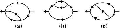
Figure 5: Two-loop diagrams contributing to the renormalization of $\Gamma_{1,1}$.

In the following we will use a compact notation for the diagrams. For example, $(\ref{ZweiLoop1}a)$ refers to diagram $(a)$ of Fig. 5. For the momentum integrals occurring in the diagrams we will use the abbreviations

$$I_{klm}=\int\limits_{\mathbf{q}_{1},\mathbf{q}_{2}}\frac{1}{\bigl{(}\mathbf{q}_{1}^{\,2}+1\bigr{)}^{k}\bigl{(}\mathbf{q}_{2}^{\,2}+1\bigr{)}^{l}\bigl{(}(\mathbf{q}_{1}+\mathbf{q}_{2})^{2}+1\bigr{)}^{m}}\,.$$ (33)

This has the benefit that we can write the divergent parts of the diagrams in a compact form. For the self-energy we have

$$(\ref{ZweiLoop1}a) =-\frac{g}{2}\tau^{-\varepsilon}\biggl{(}I_{112}\tau-\frac{d-4}{d}I_{113}\mathbf{q}^{2}\biggr{)}\,,$$ (34a)

$$(\ref{ZweiLoop1}b) =\frac{f^{2}}{2}\tau^{-\varepsilon}I_{113}\,,\quad(\ref{ZweiLoop1}c)=f^{2}\tau^{-\varepsilon}I_{122}\,.$$ (34b)

The $I_{klm}$ can be calculated very efficient with help of the parameter integral

$$I(a,b;c)=\int\limits_{\mathbf{q}_{1},\mathbf{q}_{2}}\frac{1}{\bigl{(}\mathbf{q}_{1}^{\,2}+a\bigr{)}\bigl{(}\mathbf{q}_{2}^{\,2}+b\bigr{)}\bigl{(}(\mathbf{q}_{1}+\mathbf{q}_{2})^{2}+c\bigr{)}^{2}}\,.$$ (35)

Using dimensional regularization, we find the $\varepsilon$ expansion result

$$I(a,b;c)=-\frac{2\pi G_{\varepsilon}^{2}}{3\varepsilon}\,(a+b-c)+O(\varepsilon^{0})$$ (36)

for the parameter integral. This calculation is sketched in the Appendix. In Eq. (36) we used the shorthand $G_{\varepsilon}=\Gamma(1+\varepsilon/2)/(4\pi)^{d/2}$ for convenience. By taking derivatives with respect to the parameters $a$, $b$ and $c$, we get the singular parts

$$I_{122}=-I_{112}=-2I_{113}=\frac{2\pi G_{\varepsilon}^{2}}{3\varepsilon}$$ (37)

of the required original integrals. Collecting we find

$$\Gamma_{1,1} =(\tau+\mathbf{q}^{2})-(\ref{ZweiLoop1}a)-(\ref{ZweiLoop1}b)-(\ref{ZweiLoop1}c)$$

$$=\biggl{(}1-\frac{A_{\varepsilon}g}{\varepsilon}\tau^{-\varepsilon}\biggr{)}\tau-\frac{3A_{\varepsilon}f^{2}}{2\varepsilon}\tau^{-\varepsilon}$$

$$+\biggl{(}1+\frac{A_{\varepsilon}g}{10\varepsilon}\tau^{-\varepsilon}\biggr{)}\mathbf{q}^{2}$$ (38)

for the singular part of the inverse response function. Here, we introduced $A_{\varepsilon}=\pi G_{\varepsilon}^{2}/3$ for notational convenience.

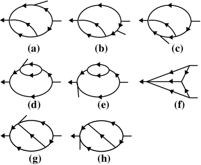
Figure 6: Two-loop diagrams contributing to the renormalization of $\Gamma_{1,2}$.

Now we turn to the vertex function $\Gamma_{1,2}$. Its two-loop contributions are shown in Fig. 6. We obtain

$$(\ref{ZweiLoop2}a) =(\ref{ZweiLoop2}b)=(\ref{ZweiLoop2}e)=(\ref{ZweiLoop2}f)=fg\tau^{-\varepsilon}I_{113}\,,$$ (39a)

$$(\ref{ZweiLoop2}c) =2\cdot(\ref{ZweiLoop2}d)=(\ref{ZweiLoop2}g)=(\ref{ZweiLoop2}h)=2fg\tau^{-\varepsilon}I_{122}\,.$$ (39b)

Summing up the individual terms we get

$$\Gamma_{1,2}=\biggl{(}1-\frac{10A_{\varepsilon}g}{\varepsilon}\tau^{-\varepsilon}\biggr{)}f\,.$$ (40)

For the vertex function $\Gamma_{2,1}$ we have to calculate the diagrams in Fig. 7.

Figure 7: Two-loop diagrams contributing to the renormalization of $\Gamma_{2,1}$.

With

$$(\ref{ZweiLoop3}a)=(\ref{ZweiLoop3}b)=-g\tau^{-\varepsilon}I_{113}\,,\quad(\ref{ZweiLoop3}c)=-2g\tau^{-\varepsilon}I_{122}\,,$$ (41)

we obtain

$$\Gamma_{2,1}=\biggl{(}1-\frac{2A_{\varepsilon}g}{\varepsilon}\tau^{-\varepsilon}\biggr{)}$$ (42)

It remains to consider $\Gamma_{1,3}$. The diagrams in Fig. 8 lead to

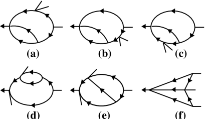
Figure 8: Two-loop diagrams contributing to the renormalization of $\Gamma_{1,3}$.

$$2\cdot(\ref{ZweiLoop4}a) =2\cdot(\ref{ZweiLoop4}b)=(\ref{ZweiLoop4}d)=3g^{2}\tau^{-\varepsilon}I_{113}\,,$$

$$2\cdot(\ref{ZweiLoop4}c) =(\ref{ZweiLoop4}e)=2\cdot(\ref{ZweiLoop4}f)=6g^{2}\tau^{-\varepsilon}I_{122}\,,$$ (43a)

From these expressions we get

$$\Gamma_{1,3}=\biggl{(}1-\frac{18A_{\varepsilon}g}{\varepsilon}\tau^{-\varepsilon}\biggr{)}g\,.$$ (44)

For completeness, we conclude our quasi-static perturbation theory by briefly returning to a cutoff regularization. In cutoff regularization there are two additional singular two-loop diagrams, see Fig. 9.

Figure 9: Two-loop diagrams that contain insertions of the one-loop diagram shown in Fig. 4(b). In dimensional regularization, these two-loop diagrams are finite.

These diagrams have divergent insertions of the singular one-loop diagram (4b). Hence, the diagrams of Fig. 9 are finite in dimensional regularization. However, in the more physical cutoff regularization they diverge linearly with the cutoff. These divergencies are ultimately cancelled by the additive renormalizations, Eq. (32).

IV.2 Renormalization

Next we absorb the $\varepsilon$-poles, into a reparametrization of the fields and the parameters of the theory. For the quasi-static fields we employ the renormalizations

$$s\rightarrow{\mathring{s}}=Z^{1/2}s\,,\quad\widetilde{s}\rightarrow{\mathring{\widetilde{s}}}=\widetilde{Z}^{1/2}\widetilde{s}\,.$$ (45)

For the parameters of the quasi-static Hamiltonian (27) we use the scheme

$$A_{\varepsilon}g\rightarrow A_{\varepsilon}{\mathring{g}}=Z_{\lambda}^{-3}\widetilde{Z}Z_{u}u\mu^{2\varepsilon}\,,$$ (46a)

$$A_{\varepsilon}^{1/2}f\rightarrow A_{\varepsilon}^{1/2}{\mathring{f}}=Z_{\lambda}^{-2}\widetilde{Z}^{1/2}Z_{v}v\mu^{\varepsilon}\,,$$ (46b)

$$\tau\rightarrow{\mathring{\tau}}=Z_{\lambda}^{-1}(Z_{\tau}\tau+Yv^{2})\,,$$ (46c)

where

$$Z_{\lambda}=(Z\widetilde{Z})^{1/2}\,.$$ (47)

It follows from Eq. (45) that the vertex functions are renormalized by

$$\Gamma_{\widetilde{N},N}\rightarrow{\mathring{\Gamma}}_{\widetilde{N},N}=\widetilde{Z}^{-\widetilde{N}/2}Z^{-N/2}\,\Gamma_{\widetilde{N},N}\,.$$ (48)

Using Eq. (48) together with our two-loop results (IV.1.2), (40), (42), and (44) we find

$$Z =1-\frac{22u}{5\varepsilon}+O(u^{2})\,,\quad\widetilde{Z}=1+\frac{21u}{5\varepsilon}+O(u^{2})\,,$$ (49a)

$$Z_{u} =1+\frac{18u}{\varepsilon}+O(u^{2})\,,\quad Z_{v}=1+\frac{10u}{\varepsilon}+O(u^{2})\,,$$ (49b)

$$Z_{\tau} =1+\frac{u}{\varepsilon}+O(u^{2})\,,\quad Y=\frac{3}{2\varepsilon}+O(u)\,,$$ (49c)

for the renormalization factors. Equation (49a) implies

$$Z_{\lambda}=1-\frac{u}{10\varepsilon}+O(u^{2})\,.$$ (50)

IV.3 Renormalization group equation

In order to explore the scaling properties of tricritical percolation we now set up a renormalization group equation (RGE). This can be done in a routine fashion by exploiting that the bare (unrenormalized) quantities must not depend on the arbitrary mesoscopic length scale $\mu^{-1}$ introduced in the course of the renormalization. In particular the bare Green functions must be independent of $\mu$, i.e.,

$$\mu\left.\partial_{\mu}\right|_{0}\mathring{G}_{N,\widetilde{N}}=0\,,$$ (51)

where $\left.\partial_{\mu}\right|_{0}$ denotes $\mu$-derivatives at fixed bare parameters. Switching from bare to renormalized quantities, the identity (51) translates into the RGE

$$\biggl{[}\mathcal{D}_{\mu}+\frac{1}{2}\bigl{(}N\gamma+\widetilde{N}\widetilde{\gamma}\bigr{)}\biggr{]}G_{N,\widetilde{N}}=0\,.$$ (52)

Here, $\mathcal{D}_{\mu}$ stands for the RG differential operator

$$\mathcal{D}_{\mu}=\mu\partial_{\mu}+\bigl{(}\tau\kappa_{\tau}+v^{2}\kappa_{v\tau}\bigr{)}\partial_{\tau}+v\kappa_{v}\partial_{v}+\beta_{u}\partial_{u}$$ (53)

that features the Gell-Mann–Low functions

$$\beta_{u}=\mu\left.\partial_{\mu}\right|_{0}u=\biggl{(}-2\varepsilon+\frac{3}{2}\gamma+\frac{1}{2}\widetilde{\gamma}-\gamma_{u}\biggr{)}u\,,$$ (54a)

$$v\kappa_{v}=\mu\left.\partial_{\mu}\right|_{0}v=\biggl{(}-\varepsilon+\gamma+\frac{1}{2}\widetilde{\gamma}-\gamma_{v}\biggr{)}v\,,$$ (54b)

$$\tau\kappa_{\tau}+v^{2}\kappa_{v\tau}=\mu\left.\partial_{\mu}\right|_{0}\tau=\biggl{(}\frac{\gamma+\widetilde{\gamma}}{2}-\gamma_{\tau}\biggr{)}\tau-\gamma_{\tau v}v^{2}\,,$$ (54c)

and the Wilson functions

$$\gamma =\mu\left.\partial_{\mu}\right|_{0}\ln Z\,,\qquad\widetilde{\gamma}=\mu\left.\partial_{\mu}\right|_{0}\ln\widetilde{Z}\,,$$ (55a)

$$\gamma_{i} =\mu\left.\partial_{\mu}\right|_{0}\ln Z_{i}\,,\quad i=u,v,\tau\,.$$ (55b)

From Eq. (54a) we know that the functions $$\beta_{u} v\kappa_{v} -2\varepsilon u -\varepsilon v \gamma_{\cdots}=\mu\left.\partial_{\mu}\right|_{0}\ln Z_{\cdots}=\beta\partial_{u}\ln Z_{\cdots} Z \varepsilon Z_{\cdots}=1+Z_{\cdots}^{(1)}/\varepsilon+Z_{\cdots}^{(2)}/\varepsilon^{2}+\cdots \varepsilon\rightarrow 0 \varepsilon \gamma_{\cdots}=-2u\partial_{u}Z^{(1)} \gamma_{\tau v}=-2Y^{(1)}-2u\partial_{u}Y^{(1)} Y^{(1)} Y=Y^{(1)}/\varepsilon+\cdots Y$$ and begin with the zero-loop terms and respectively. The higher order terms are determined by the Wilson functions. The particular form of these functions can be straightforwardly extracted by using . In minimal renormalization the -factors have a pure Laurent expansion with respect to , i.e., they are of the form . Thus, recursively in the loop expansion, the Wilson functions also have a pure Laurent expansion. Moreover, because the Wilson functions must be finite for , all the -poles in this expansion have to cancel (this provides a valuable check for higher order calculations). Hence, we can obtain the Wilson functions readily from the formula . The same argumentation also leads to , where is the coefficient of the first order term in the Laurent expansion of the -factor. Using this prescription, we derive from our renormalization factors (49) that the Wilson functions are given by

$$\gamma=\frac{44u}{5}+O(u^{2})\,, \qquad\widetilde{\gamma}=-\frac{42u}{5}+O(u^{2})\,,$$ (56a)

$$\gamma_{u}=-36u+O(u^{2})\,, \qquad\gamma_{v}=-20u+O(u^{2})\,,$$ (56b)

$$\gamma_{\tau}=-2u+O(u^{2})\,, \qquad\gamma_{\tau v}=-3+O(u)\,.$$ (56c)

From these results we get

$$\beta_{u} =\bigl{(}-2\varepsilon+45u+O(u^{2})\bigr{)}u\,,$$ (57a)

$$\kappa_{v} =-\varepsilon+\frac{123u}{5}+O(u^{2})\,,$$ (57b)

$$\kappa_{\tau} =\frac{11u}{5}+O(u^{2})\ ,\quad\kappa_{v\tau}=3+O(u)$$ (57c)

for the Gell-Mann–Low functions (54).

IV.4 Scaling properties

IV.4.1 General scaling form

Next we solve the RGE (52) by using the method of characteristics. The strategy behind this method is to introduce a single flow parameter $\ell$ that allows to re-express the partial differential equation (52) as an ordinary differential equation in terms of $\ell$. This equation then describes how the Green functions behave under a rescaling

$$\mu\rightarrow\bar{\mu}(\ell)=\mu\,\ell$$ (58)

of the inverse length scale $\mu$. The characteristic for the dimensionless coupling constant $u$ is given by

$$\ell\frac{d\bar{u}(\ell)}{d\ell}=\beta_{u}(\bar{u}(\ell))\,,\quad\bar{u}(1)=u\,.$$ (59)

With the exception of the characteristic for $\tau$, the remaining characteristics are all of the same structure, viz.

$$\ell\frac{d\ln Q(\bar{u}(\ell))}{d\ell}=q(\bar{u}(\ell))\,.$$ (60)

Here, $Q$ is a placeholder for $X$, $\widetilde{X}$, and $\bar{v}$, respectively. $q$ is a placeholder for respectively $\gamma$, $\widetilde{\gamma}$, and $\kappa_{v}$. The initial conditions pertaining to Eq. (60) are $X(1)=\widetilde{X}(1)=1$ and $\bar{v}(1)=v$. The long-length scale behavior of TIP corresponds to the limit $\ell\to 0$. In this limit the RG flows to a fixed point determined by the stable value $u_{\ast}$ of $u$ satisfying $\beta_{u}(u_{\ast})=0$. We find that this value is given by $u_{\ast}=2\varepsilon/45+O(\varepsilon^{2})$.

For the remainder of Sec. IV.4 we exclusively consider dimensions less than 5. We will turn to the case $d=5$ in Sec. IV.5. In the vicinity of the fixed point $u_{\ast}$ the solution of the RGE with the characteristics is fairly straightforward. We are confronted, however, with the slight complication that $\tau$ itself is not a scaling variable as can be seen from Eq. (54c). In order to diagonalize the flow equations in near $u_{\ast}$ we switch from $\tau$ to

$$\sigma=\tau+\frac{\kappa_{v\tau\ast}}{\kappa_{\tau\ast}-2\kappa_{v\ast}}\,v^{2}\,,$$ (61)

where $\kappa_{\tau\ast}=\kappa_{\tau}(u_{\ast})$, $\kappa_{v\ast}=\kappa_{v}(u_{\ast})$ and so on. It can easily be checked that $\sigma$ is governed by the flow equation

$$\ell\frac{d\ln\sigma(\ell)}{d\ell}=\kappa_{\tau\ast}\,,$$ (62)

i.e, that $\sigma$ is a true scaling variable. In the dimensions of interest here the solutions of the characteristics for the scaling variables are of power law form and we obtain

$$G_{N,\widetilde{N}}(\{\mathbf{r}\},\tau,v,u,\mu)=\ell^{(N\eta+\widetilde{N}\widetilde{\eta})/2}$$

$$\qquad\qquad\times\bar{G}_{N,\widetilde{N}}(\{\mathbf{r}\},\sigma\ell^{\kappa_{1}},v\ell^{\kappa_{2}},u_{\ast},\mu\ell)\,,\,$$ (63)

where we have omitted nonuniversal amplitude factors. The various exponents appearing in Eq. (63) are given by

$$\eta =\gamma(u_{\ast})=\frac{88}{225}\varepsilon+O(\varepsilon^{2})\,,$$ (64a)

$$\widetilde{\eta} =\widetilde{\gamma}(u_{\ast})=-\frac{28}{75}\varepsilon+O(\varepsilon^{2})\,,$$ (64b)

$$\kappa_{1} =\kappa_{\tau}(u_{\ast})=\frac{22}{225}\varepsilon+O(\varepsilon^{2})\,,$$ (64c)

$$\kappa_{2} =\kappa_{v}(u_{\ast})=\frac{7}{75}\varepsilon+O(\varepsilon^{2})\,.$$ (64d)

Supplementing the solution (63) with a dimensional analysis to account for naive dimensions we obtain the scaling form

$$G_{N,\widetilde{N}}(\{\mathbf{r}\},\tau,v,u,\mu)=\ell^{\delta_{N,\widetilde{N}}}\mu^{(d-4)N+2\widetilde{N}}$$

$$\qquad\times F_{N,\widetilde{N}}(\{\ell\mu\mathbf{r}\},\mu^{-2}\sigma/\ell^{1/\nu},\mu^{-1}v/\ell^{\phi/\nu})\,,$$ (65)

where

$$\delta_{N,\widetilde{N}}=\Bigl{(}d-4+\frac{\eta}{2}\Bigr{)}N+\Bigl{(}2+\frac{\widetilde{\eta}}{2}\Bigr{)}\widetilde{N}\,,$$

and where the $F_{N,\widetilde{N}}$ are, up to nonuniversal amplitude factors, universal scaling functions. The scaling exponents of the correlation length and the crossover variable are

$$\nu =\frac{1}{2-\kappa_{1}}=\frac{1}{2}+\frac{11}{450}\varepsilon+O(\varepsilon^{2})\,,$$ (66a)

$$\phi =\frac{1-\kappa_{2}}{2-\kappa_{1}}=\frac{1}{2}-\frac{1}{45}\varepsilon+O(\varepsilon^{2})\,.$$ (66b)

In the following we will concentrate on a path in the phase diagram spanned by the relevant variables $\tau$ and $v$ which approaches the tricritical point $\tau=v=0$ as $v\sim\tau$. Hence, we will neglect the crossover variable $v/\left|\sigma\right|^{\phi}\sim\left|\tau\right|^{1-\phi}\ll 1$, where we have set $\mu=1$ for convenience. In this regime we can write the fundamental scaling form (IV.4.1) as

$$G_{N,\widetilde{N}}(\{\mathbf{r}\},\tau)=\left|\tau\right|^{N\beta+\widetilde{N}{\beta}^{\prime}}F_{N,\widetilde{N}}^{\pm}(\{\left|\tau\right|^{\nu}\mathbf{r}\})\,,$$ (67)

with

$$\beta =\nu\Bigl{(}d-4+\frac{\eta}{2}\Bigr{)}=\frac{1}{2}-\frac{17}{45}\varepsilon+O(\varepsilon^{2})\,,$$ (68a)

$${\beta}^{\prime} =\nu\Bigl{(}2+\frac{\widetilde{\eta}}{2}\Bigr{)}=1-\frac{2}{45}\varepsilon+O(\varepsilon^{2})\,.$$ (68b)

The superscript of the scaling functions $$F_{N,\widetilde{N}}^{\pm} \tau \xi\sim\left|\tau\right|^{-\nu}$$ corresponds to the sign of . Note that is the correlation length.

IV.4.2 Scaling behavior of various percolation observables

Now we will exploit our knowledge about the correlation functions of the fields to extract the scaling behavior of various observables that play an important role in percolation theory. First we will consider the case that the process starts with a single seed at the origin $\mathbf{r}=0$. Second we will look at the case that the density of the initial state is homogeneous.

Let us start by considering clusters of a given finite size $S$, i.e. clusters with a finite mass $S$ of the debris given that the process started with a seed, a single agent, at the origin $\mathbf{r}=0$. In principle, any reasonable initial state can be prepared by choosing the appropriate seed density $\rho_{0}(\mathbf{r})$. In the Langevin equation (17) this general initial condition corresponds to an additional source term $\lambda^{-1}{q}(\mathbf{r},t)=\rho_{0}(\mathbf{r})\,\delta(\lambda t)$. At the level of the dynamic response functional $\mathcal{J}$ (23) such an initial state translates into a further additive contribution $-\int d^{d}x\,dt\,q(\mathbf{r},t)\tilde{n}(\mathbf{r},t)$. Thus, a seed $q(\mathbf{r},t)=\delta(\mathbf{r})\delta(t)$ is represented by the contribution $-\tilde{n}(\mathbf{0},0)$. At the level of the quasistatic Hamiltonian $\mathcal{H}$ (27) such a seed is therefore represented by an additive term $-\tilde{s}(0)$.

Let $P(S)dS$ be the measure for the probability that the cluster mass of the debris generated by a seed at the origin is between $S$ and $S+dS$. In our field theoretic formulation the probability density $P(S)$ can be expressed as

$$P(S)=\left\langle\delta\Bigl{(}\int d^{d}r\,s(\mathbf{r})-S\Bigr{)}\,\exp\left[\tilde{s}(\mathbf{0})\right]\right\rangle\,.$$ (69)

For big clusters with $S\gg 1$ we can expand the exponential to first order (higher orders lead asymptotically only to subleading corrections) and obtain

$$P_{\text{as}}(S)=\left\langle\delta\Bigl{(}\int d^{d}r\,s(\mathbf{r})-S\Bigr{)}\,\,\tilde{s}(\mathbf{0})\right\rangle\,$$ (70)

for the asymptotic distribution. We will return to $P_{\text{as}}(S)$ in a moment.

The percolation probability $\mathcal{P}_{\infty}$ is defined as the probability for the existence of an infinite cluster generated from a single seed. Hence $\mathcal{P}_{\infty}$ is given by

$$\mathcal{P}_{\infty} =1-\lim_{c\rightarrow+0}\int_{0}^{\infty}dS\,\mathrm{e}^{-cS}P(S)$$

$$=1-\lim_{c\rightarrow+0}\langle\exp\Big{(}\widetilde{s}(\mathbf{0})-c\int d^{d}r\,s(\mathbf{r})\Big{)}\rangle.$$ (71)

Via expanding $\exp[\tilde{s}(\mathbf{0})]$ we obtain the asymptotic form Ja03

$$\mathcal{P}_{\infty}\simeq-\lim_{c\rightarrow+0}\langle\tilde{s}(\mathbf{0})\mathrm{e}^{-cM}\rangle\,,$$ (72)

where $M=\int d^{d}x\,s(\mathbf{x})$. The virtue of this formula is that it relates the percolation probability unambiguously to an expression accessible by field theory. For actual calculations the term $\exp(-cM)$ has to be incorporated into the quasi-static Hamiltonian. This leads to

$$\mathcal{H}_{c}=\mathcal{H}+\int d^{d}r\,c(\mathbf{r})s(\mathbf{r})$$ (73)

instead of the original $\mathcal{H}$. Here, $c(\mathbf{x})=c$ is a source conjugate to the field $s$. Whereas in general $\langle\tilde{s}\rangle=0$ if $c=0$ by virtue of causality, the limit $c\rightarrow+0$ leads to a nonvanishing order parameter $\mathcal{P}_{\infty}$ in the spontaneously symmetry broken active phase. Having introduced $\mathcal{H}_{c}$, we can write

$$\mathcal{P}_{\infty} =-\lim_{c\rightarrow+0}\langle\tilde{s}(\mathbf{0})\rangle_{c}$$

$$=-G_{0,1}(\mathbf{0},\tau,c\rightarrow+0,u,\mu)\,,$$ (74)

where $\langle\cdots\rangle_{c}$ denotes averaging with respect to $\mathcal{H}_{c}$. With the help of Eq. (74) and the scaling form (67) we readily obtain that

$$\mathcal{P}_{\infty}\sim\theta(-\tau)\left|\tau\right|^{\beta^{\prime}}\,.$$ (75)

In order to examine the scaling behavior of $P(S)$ we can look at its moments defined by

$$\langle S^{k}\rangle=\int_{0}^{\infty}dS\,S^{k}P(S)\,.$$ (76)

Using Eq. (70), our scaling result (67) leads to

$$\langle S^{k}\rangle\simeq\int(d^{d}r)^{k}\,G_{k,1}(\{\mathbf{r}\},\mathbf{0},\tau)\sim\left|\tau\right|^{{\beta}^{\prime}-k(d\nu-\beta)}\,.$$ (77)

This tells us that $P_{\text{as}}$ scales as

$$P_{\text{as}}(S,\tau)=S\,n_{S}(\tau)=S^{1-\tau_{p}}f(\tau S^{\sigma_{p}})\,,$$ (78)

where $n_{S}$ is the number of clusters of size $S$ per lattice site. The $n_{S}$ play an important role in percolation theory where they are called cluster numbers. The scaling exponents in the scaling form (77) reflect the usual nomenclature of percolation theory. They are given by

$$\sigma_{p} =\frac{1}{d\nu-\beta}=\frac{1}{2}+O(\varepsilon^{2})\,,$$ (79a)

$$\tau_{p} =\frac{{\beta}^{\prime}}{d\nu-\beta}+2=\frac{5}{2}-\frac{1}{45}\varepsilon+O(\varepsilon^{2})\,.$$ (79b)

These exponents coincide with the corresponding exponents of conventional isotropic percolation only in mean-field theory. It follows from Eq. (77) that the mean cluster mass $$\langle S\rangle$$ of the finite clusters scales as

$$\langle S\rangle=\mathcal{M}(\tau)=\mathcal{M}_{0}\,\left|\tau\right|^{-\gamma},$$ (80)

with the exponent

$$\gamma=d\nu-(\beta+{\beta}^{\prime})=1+\frac{2}{45}\varepsilon+O(\varepsilon^{2})\,.$$ (81)

Next we consider Green functions restricted to clusters of given mass $S$. In terms of the conventional unrestricted averages with respect to $\mathcal{H}$, these restricted Green functions can be expressed for large $S$ as

$$C_{N}^{(S)}(\{\mathbf{r}\},\tau)$$

$$=\left\langle s(\mathbf{r}_{1})\cdots s(\mathbf{r}_{N})\delta\Bigl{(}\int d^{d}r\,s(\mathbf{r})-S\Bigr{)}\widetilde{s}(\mathbf{0})\right\rangle^{(\text{conn})}\,.$$ (82)

Equation (67) leads to the scaling form

$$C_{N}^{(S)}(\{\mathbf{r}\},\tau)=\left|\tau\right|^{(N-1)\beta+\beta^{\prime}+d\nu}F_{N}(\{\left|\tau\right|^{\nu}\mathbf{r}\},\left|\tau\right|^{d\nu-\beta}S)\,.$$ (83)

With help of these restricted Green functions we can write the radius of gyration (mean-square cluster radius) of clusters of size $S$ as

$$R_{S}^{2}=\frac{\int d^{d}r\,\mathbf{r}^{2}C_{1}^{(S)}(\mathbf{r,\tau})}{2d\int d^{d}r\,C_{1}^{(S)}(\mathbf{r,\tau})}\,.$$ (84)

Equation (83) then leads to

$$R_{S}^{2}=S^{2/D_{f}}f_{R}(\tau S^{\sigma_{p}})\$$ (85)

with the fractal dimension

$$D_{f}=d-\frac{\beta}{\nu}=4-\frac{44}{225}\varepsilon+O(\varepsilon^{2})\ .$$ (86)

We conclude Sec. IV by considering the scaling behavior of the statistics of the debris if the initial state is prepared with a homogeneous seed density $\rho_{0}$. As discussed above, such an initial state translates at the level of the quasistatic Hamiltonian $\mathcal{H}$ (27) into a further additive contribution $-\rho_{0}\int d^{d}r\,\widetilde{s}(\mathbf{r})$. Our general scaling form (67) implies that the correlation functions of the densities $s(\mathbf{r})$ scale in case of the homogeneous initial condition like

$$G_{N,\tilde{N}}(\{\mathbf{r}\},\tau,\rho_{0}) =\sum_{k=0}^{\infty}\frac{\rho_{0}^{k}}{k!}\int(d^{d}\widetilde{r})^{k}\,G_{N,\widetilde{N}+k}(\{\mathbf{r}\},\{\widetilde{\mathbf{r}}\},\tau)$$

$$=\left|\tau\right|^{\beta N+\beta^{\prime}\tilde{N}}F_{N}^{\pm}(\{\left|\tau\right|^{\nu}\mathbf{r}\},\left|\tau\right|^{{\beta}^{\prime}-d\nu}\rho_{0})\ .$$ (87)

It is obvious that the initial seed density plays the role of an ordering field. Hence, the Green functions do not show critical singularities as long as $\rho_{0}$ is finite. For the homogeneous initial condition the appropriate order parameter is given by the density of the debris

$$\rho=\langle s(\mathbf{r})\rangle_{\rho_{0}}=G_{1,0}(\mathbf{r},\tau,\rho_{0})\,.$$ (88)

Equation (87) tells us that

$$\rho=\left|\tau\right|^{\beta}f_{\rho}^{\pm}(\left|\tau\right|^{{\beta}^{\prime}-d\nu}\rho_{0})\,.$$ (89)

In the non-percolating phase ($\tau>0$) the order parameter $\rho$ is linear in $\rho_{0}$ for small seed density with a susceptibility coefficient that diverges as $\tau\rightarrow 0$,

$$\rho(\tau>0,\rho_{0})\sim\tau^{-\gamma}\rho_{0}\,,$$ (90)

with the susceptibility exponent $\gamma$ given in Eq. (81). At criticality ($\tau=0$) the order parameter $\rho$ goes to zero for $\rho_{0}\rightarrow 0$ as

$$\rho(\tau=0,\rho_{0})\sim\rho_{0}^{1/\delta}\,,$$ (91)

with the exponent

$$\delta=\frac{d\nu-{\beta}^{\prime}}{\beta}=1+\frac{\gamma}{\beta}=3+\frac{8}{5}\varepsilon+O(\varepsilon^{2})\,.$$ (92)

Finally, in the percolating phase ($\tau<0$) the order parameter becomes independent of the initial seed density in the limit $\rho_{0}\rightarrow 0$ and goes to zero with $\tau$ as

$$\rho(\tau<0)\sim\left|\tau\right|^{\beta}\,.$$ (93)

Equations (75) and (93) show explicitly that the two order parameters, namely the density $\rho$ of the debris and the percolation probability $\mathcal{P}_{\infty}$, have different exponents $\beta$ and ${\beta}^{\prime}$. This stands in contrast to ordinary isotropic as well as directed percolation. As mentioned earlier, ordinary isotropic and directed percolation are special in the sense that they posses an asymptotic symmetry that leads to the equality of the respective exponents $\beta$ and ${\beta}^{\prime}$.

IV.5 Scaling properties in 5 dimensions – logarithmic corrections

Here we will study TIP directly in 5 dimensions where fluctuations induce logarithmic corrections to the leading mean-field terms rather than anomalous exponents. First, we will establish the general form of the logarithmic corrections. Second, we will analyze how these corrections, to leading order, affect the observables studied in Sec. IV.4

IV.5.1 General form of the logarithmic corrections

Now we will solve the characteristics directly for $d=5$. The Wilson functions stated in Eqs. (56) and (57) are central ingredients of the characteristics. For ecconomic reasons, we will use in the following an abbreviated notion for the Wilson functions of the type $f(u)=f_{1}u+f_{2}u^{2}+\cdots$. For instance, we will write Eq. (57a) as $\beta_{u}(u)=\beta_{1}u+\beta_{2}u^{2}+O(u^{3})$ and likewise for the other Wilson functions. Since we are interested in the tricritical point, we set $v=0$ throughout.

Solving the characteristic for $u$, Eq. (59), for $\varepsilon=0$ yields readily

$$\ell=\ell(w)=\ell_{0}\exp\bigg{[}-\frac{1}{\beta_{2}w}+O(\ln w)\bigg{]}\,,$$ (94)

where $\ell_{0}$ is an integration constant and where we abbreviated

$$w=\bar{u}\,.$$ (95)

To leading order we obtain from Eq. (94) asymptotically for $\ell\ll 1$

$$w\simeq\frac{1}{45\left|\ln\ell\right|}\ll 1.$$ (96)

The remaining characteristics, Eq. (60) are solved via exploiting $\ell d/d\ell=\beta d/dw$ with the asymptotic result

$$Q(w)\simeq Q_{0}\,w^{q_{1}/\beta_{2}}\,,$$ (97)

where $Q_{0}$ symbolizes a non-universal integration constant. Having solved the characteristics, we obtain

$$G_{N,\widetilde{N}}(\left\{\mathbf{r}\right\},\tau) =[\mu\ell\,X(w)^{1/2}]^{N}[(\mu\ell)^{2}\tilde{X}(w)^{1/2}]^{\widetilde{N}}$$

$$\times F_{N,\widetilde{N}}\Big{(}\left\{\mu\ell\mathbf{r}\right\},\frac{\tau(w)}{(\mu\ell)^{2}},w\Big{)}$$ (98)

as a formal scaling solution for the Green functions.

In the following we have to be careful about the explicit dependence of the scaling functions $F_{N,\widetilde{N}}$ on $w$ even though we are only interested in the leading logarithmic corrections. This intricacy comes from the fact that rather mean-field than Gaussian theory applies at the upper critical dimension. Hence we must carefully distinguish between the 2 roles of $g$, viz. its role as a dangerous irrelevant variable which scales the fields and the parameters in the correlation and response functions, and, its role (in its dimensionless form $u$) as the loop expansion parameter. Only the latter role can be safely neglected for the leading logarithmic corrections. As we shall see in the following, the dependence of the functions $F_{N,\widetilde{N}}$ on $w$ if given by

$$F_{N,\widetilde{N}}\left(\left\{\mathbf{r}\right\},\tau,v,w\right)$$

$$=w^{(1-\tilde{N})/2}\Bigl{[}F_{N,\widetilde{N}}^{\prime}\left(\left\{\mathbf{r}\right\},\tau,v/\sqrt{w}\right)+O(\sqrt{w})\Bigr{]}.$$ (99)

To derive this result one can consider the loop-scaling of the generating functionals of the vertex and Green functions as it was done in Ref. JaSt04 for studying logarithmic corrections in DP. Here we use a more direct method to determine the dependence of the tree diagrams on the dangerous variable $g$. Consider an arbitrary connected diagram with $L$ loops, $P$ propagators, $N$ external $s$-legs, $\tilde{N}$ external $\tilde{s}$-legs, $V_{g}$ vertices of type $g$, $V_{f}$ vertices of type $f$, and $V_{1}$ noise vertices proportional to $1$. This generic diagram contributing to the Green function $G_{N,\tilde{N}}$ satisfies the three topological conditions

$$L =P-V_{g}-V_{f}-V_{1}-N-\tilde{N}+1,$$ (100a)

$$P =3V_{g}+2V_{f}+V_{1}+N,$$ (100b)

$$P =V_{g}+V_{f}+2V_{1}+\tilde{N}.$$ (100c)

Eliminating $$P$$ we arrive at two equations for the number of vertices, namely

$$V_{1} =N-1+L,$$ (101a)

$$2V_{g}+V_{f} =\tilde{N}-1+L.$$ (101b)

Switching from $$f f^{\prime}=f/\sqrt{g} g g^{(\tilde{N}-1+L)/2} g^{L/2} L=0$$ to the scaled variable , we find that the diagram scales with as with the factor being determined by the loop-order of the diagram. Upon renormalization this reasoning leads for to the scaling form (99).

Knowing Eq. (99) we can write down the scaling form of the Green functions with its leading logarithmic corrections. From the general solution of the RGE for the Green functions (98) in conjunction with the asymptotic result (96) we get

$$G_{N,\widetilde{N}}(\left\{\mathbf{r}\right\},\tau) =\ell^{N+2\tilde{N}}\left|\ln\ell\right|^{7\tilde{N}/75-22N/225+(1-\tilde{N})/2}$$

$$\times F_{N,\tilde{N}}\bigl{(}\{\ell\mathbf{r}\},\ell^{-2}\left|\ln\ell\right|^{-11/225}\tau\bigr{)}.$$ (102)

IV.5.2 Logarithmic corrections to the percolation observables

As above we will first consider the case that the process emanates from a single local seed at the origin. Exploiting Eq. (74), we find that the percolation probability has the scaling form

$$\mathcal{P}_{\infty}=\ell^{2}\left|\ln\ell\right|^{7/75}f_{\mathcal{P}_{\infty}}(\ell^{-2}\left|\ln\ell\right|^{-11/225}\tau),$$ (103)

where $f_{\mathcal{P}_{\infty}}$ is non zero only for $\tau<0$. Now we fix the arbitrary but small flow parameter $\ell$ so that $\tau^{-1}$ effectively acquires a finite value in the scaling limit,

$$\ell^{-2}\left|\ln\ell\right|^{-11/225}\tau\sim 1.$$ (104)

Hence, we choose asymptotically

$$\ell^{2}\sim\left|\tau\right|\left|\ln\left|\tau\right|\right|^{-11/225}.$$ (105)

Collecting, we obtain that

$$\mathcal{P}_{\infty}(\tau)\sim\theta(-\tau)\left|\tau\right|\left|\ln\left|\tau\right|\right|^{2/45}.$$ (106)

Next we consider the probability $P(S,\tau)$. Using the definition (77) and the general result (102) we obtain

$$P(S,\tau) =\ell^{6}\left|\ln\ell\right|^{43/225}$$

$$\times f_{P}^{\prime}\bigl{(}\ell^{-2}\left|\ln\ell\right|^{-11/225}\tau,\ell^{4}\left|\ln\ell\right|^{22/225}S\bigr{)}\,.$$ (107)

Being interested primarily in $P(S,\tau)$ as a function near criticality $\tau\approx 0$ and not in the animal limit $S\rightarrow\infty$ with $\tau>0$, we hold the second argument finite. Hence we choose

$$\ell^{4}\sim S^{-1}(\ln S)^{-22/225}\,.$$ (108)

With these settings we find

$$P(S,\tau)=S^{-3/2}\,(\ln S)^{2/45}\,f_{P}\bigl{(}\tau S^{1/2}\bigr{)}.$$ (109)

The scaling function $\,f_{P}\left(x\right)$ is found with help of a simple mean field calculation to be proportional to $\exp(-\mathrm{const}\,x^{2})\,$as long as $x$ is finite. For $x\rightarrow\infty$ it crosses over to the animal limit with its own independent scaling behavior. Note that there is, to the order we are working, no logarithmic correction associated with the $S^{1/2}$ in the argument of the scaling function. As a corollary of Eq. (109), we obtain the critical behavior of the mean cluster mass,

$$\mathcal{M(\tau)}=\langle S\rangle\sim\tau^{-1}\,\left|\ln\tau\right|^{2/45}.$$ (110)

Now we turn to clusters of a given size $S$. The scaling behavior of the Green functions restricted to these clusters takes on the form

$$C_{N}^{(S)}(\{\mathbf{r}\},\tau)=\ell^{N+6}\left|\ln\ell\right|^{(43-22N)/225}$$

$$\times F_{N}\bigl{(}\left\{\ell\mathbf{r}\right\},\ell^{-2}\left|\ln\ell\right|^{-11/225}\tau,\ell^{4}\left|\ln\ell\right|^{22/225}S\bigr{)}$$ (111)

in 5 dimensions. From this scaling it is straightforward to extract the radius of gyration of clusters of size $S$ via definition (84). Choosing $\ell$ per Eq. (108) leads to

$$R_{S}^{2}=S^{1/2}\,(\ln S)^{11/225}\,f_{R}\bigl{(}\tau S^{1/2}\bigr{)}.$$ (112)

In mean-field theory, as a straightforward calculation shows, the scaling function $f_{R}(x)$ is identical to a non-universal constant.

In the remainder of Sec. IV.5 we will consider the homogeneous initial condition. The $N$-point density correlation functions obey in $d=5$ the scaling form

$$G_{N,\tilde{N}}(\{\mathbf{r}\},\tau,\rho_{0})=\ell\,^{N+2\tilde{N}}\left|\ln\ell\right|^{1/2+61\tilde{N}/150-22N/225}$$

$$\times F_{N,\tilde{N}}\bigl{(}\left\{\ell\mathbf{r}\right\},\ell^{-2}\left|\ln\ell\right|^{-11/225}\tau,\ell^{-3}\left|\ln\ell\right|^{-61/150}\rho_{0}\bigr{)}.$$ (113)

Specifying Eq. (113) to $N=1$ and $\tilde{N}=0$, we obtain the scaling behavior of the mean density of the debris,

$$\bar{\rho}(\tau,\rho_{0})=\ell\left|\ln\ell\right|^{181/450}$$

$$\times F_{1,0}\bigl{(}\ell^{-2}\left|\ln\ell\right|^{-11/225}\tau,\ell^{-3}\left|\ln\ell\right|^{-61/150}\rho_{0}\bigr{)}.$$ (114)

For $\tau\neq 0$ and small seed density $\rho_{0}$ it is appropriate to choose $\ell$ according to Eq. (104). This provides us with

$$\bar{\rho}(\tau,\rho_{0})=\left|\tau\right|^{1/2}\,\left|\ln\left|\tau\right|\right|^{17/45}\,f_{\bar{\rho}}^{\pm}\bigl{(}\rho_{0}\,\left|\tau\right|^{-3/2}\,\left|\ln\left|\tau\right|\right|^{-1/3}\bigr{)}\,.$$ (115)

The scaling function $f_{\bar{\rho}}^{+}(x)$ behaves like $f_{\bar{\rho}}^{+}(x)\sim x$ for small $x$, and hence

$$\bar{\rho}(\tau>0,\rho_{0})\sim\rho_{0}\,\tau^{-1}\,\left|\ln\tau\right|^{2/45}$$ (116)

in this regime. At $\tau=0$, the mean density is a function of $\rho_{0}$ only. To obtain the logarithmic corrections for this case, we set

$$\ell\sim\rho_{0}\,^{1/3}\,\left|\ln\rho_{0}\right|^{-61/450}.$$ (117)

From Eq. (114) in conjunction with Eq. (117) we obtain

$$\bar{\rho}(\tau=0,\rho_{0})\sim\rho_{0}^{1/3}\,\left|\ln\rho_{0}\right|^{4/15}\,.$$ (118)

Lastly, the order parameter should be independent of the seed density in the percolating phase for $\rho_{0}\rightarrow 0$, i.e., the scaling function $f_{\bar{\rho}}^{-}$ of Eq. (115) should approach a constant in this limit. Thus, we get

$$\bar{\rho}(\tau<0)\sim\left|\tau\right|^{1/2}\,\left|\ln\left|\tau\right|\right|^{17/45}$$ (119)

in this regime.

V Dynamic Scaling Properties

In this section we will study dynamic scaling properties of TdIP. To find out these properties we have to renormalize the dynamic response functional (23). In comparison to the quasi-static Hamiltonian (27), $\mathcal{J}$ has one additional parameter, namely the kinetic coefficient $\lambda$. To determine the renormalization of $\lambda$, we have to calculate one of the dynamic vertex functions in full time or frequency dependence. A dynamic RGE then leads to general scaling form for the dynamic Green functions. This scaling form allows us to deduce the dynamic scaling behavior of various percolation observables.

V.1 Diagrammatics

In order to determine the renormalization of $\lambda$, we could calculate the frequency dependent part of any of the superficially divergent vertex functions. For convenience, we choose to work with $\Gamma_{1,1}$. Two dynamic two-loop diagrams for the self-energy can be constructed from the diagrammatic elements in Fig. 2. These two diagrams are shown in Fig. 10.

Figure 10: Dynamic two-loop diagrams which provide us with the renormalization factor of the kinetic coefficient $\lambda$.

After Fourier transformation and some rearrangements, we get from the diagrams the contribution

$$(\ref{DynGraph}a)+(\ref{DynGraph}b)=i\omega g\tau^{-\varepsilon}\biggl{(}-\frac{B}{8}+\frac{C}{2}+\frac{3}{8}I_{122}+\frac{3}{4}I_{113}\biggr{)}$$ (120)

to $\Gamma_{1,1}$, where we have not displayed various terms (those not linear in the frequency $\omega$) for notational simplicity. $B$ and $C$ stand for the integrals

$$B=\int\limits_{\mathbf{q}_{1},\mathbf{q}_{2}}\frac{1}{\bigl{(}\mathbf{q}_{1}^{\,2}+1\bigr{)}^{2}\bigl{(}\mathbf{q}_{2}^{\,2}+1\bigr{)}^{2}\bigl{(}\mathbf{q}_{1}^{\,2}+\mathbf{q}_{2}^{\,2}+(\mathbf{q}_{1}+\mathbf{q}_{2})^{2}+3\bigr{)}}$$ (121)

and

$$C=\int\limits_{\mathbf{q}_{1},\mathbf{q}_{2}}\frac{1}{\bigl{(}\mathbf{q}_{1}^{\,2}+1\bigr{)}^{2}\bigl{(}\mathbf{q}_{2}^{\,2}+1\bigr{)}^{2}\bigl{(}\mathbf{q}_{1}^{\,2}+(\mathbf{q}_{1}+\mathbf{q}_{2})^{2}+2\bigr{)}}\,.$$ (122)

These integrals can be calculated for example by using Schwinger parametrization, cf. the appendix. The $\varepsilon$ expansion results for $B$ and $C$ read,

$$B=\frac{4G_{\varepsilon}^{2}}{9\varepsilon}\bigl{(}3\sqrt{3}-\pi\bigr{)}\,,\quad C=\frac{4G_{\varepsilon}^{2}}{3\varepsilon}\,.$$ (123)

The $I_{\cdots}$-contributions in Eq. (120) cancel and we finally get

$$(\ref{DynGraph}a)+(\ref{DynGraph}b)=\frac{i\omega G_{\varepsilon}^{2}g\tau^{-\varepsilon}}{3\varepsilon}\biggl{(}2-\frac{\sqrt{3}}{2}+\frac{\pi}{6}\biggr{)}\ .$$ (124)

V.2 Renormalization and renormalization group equation

The dynamic theory requires an additional renormalization factor, say $Z^{\prime}$, in comparison to the quasi-static theory due to the existence of $\varepsilon$ poles in the frequency dependent terms. Taking into account that the dynamic fields $n$ and $\widetilde{n}$ are related to the quasi-static fields $s$ and $\widetilde{s}$ via Eq. (26), we introduce $Z^{\prime}$ consistent with the renormalization scheme in Eqs. (45) and (46) by letting

$$n\rightarrow{\mathring{n}}=Z^{\prime 1/2}n\,,\quad\lambda\rightarrow{\mathring{\lambda}}=(Z/Z^{\prime})^{1/2}\lambda\,.$$ (125)

Combining Eq. (124) with the zero-loop part of the vertex function $\Gamma_{1,1}$ we get by applying our renormalizations

$$\Gamma_{1,1}=i\omega\biggl{[}\bigl{(}Z^{\prime}\widetilde{Z}\bigr{)}^{1/2}-\frac{u}{6\varepsilon}\biggl{(}1+\frac{12-3\sqrt{3}}{\pi}\biggr{)}+O(u^{2})\biggr{]}\,.$$ (126)

To keep the formula (126) simple, we have once more dropped all terms which are not linear in $\omega$. From Eq. (126) we can directly read off $(Z^{\prime}\widetilde{Z})^{1/2}$ to order $u$. Taking into account Eq. (49), this yields

$$Z^{\prime}=1+\frac{u}{\varepsilon}\biggl{(}\frac{4-\sqrt{3}}{\pi}-\frac{58}{15}\biggr{)}+O(u^{2})\ .$$ (127)

The corresponding Wilson function reads

$$\gamma^{\prime}=2\biggl{(}\frac{58}{15}-\frac{4-\sqrt{3}}{\pi}\biggr{)}u+O(u^{2})\,.$$ (128)

Now we have all the information required to calculate the Gell-Mann–Low function

$$\zeta=\mu\left.\partial_{\mu}\right|_{0}\ln\lambda=\frac{1}{2}\bigl{(}\gamma^{\prime}-\gamma\bigr{)}$$ (129)

for the kinetic coefficient.

By proceeding analogous to the quasi-static case we obtain the dynamic RGE

$$\biggl{[}\mathcal{D}_{\mu}+\frac{1}{2}\bigl{(}N\gamma^{\prime}+\widetilde{N}\widetilde{\gamma}\bigr{)}\biggr{]}G_{N,\widetilde{N}}(\{\mathbf{r},t\},\tau)=0\,.$$ (130)

Here, the RG differential operator $\mathcal{D}_{\mu}$ is given by

$$\mathcal{D}_{\mu}=\mu\partial_{\mu}+\lambda\zeta\partial_{\lambda}+\bigl{(}\tau\kappa_{\tau}+v^{2}\kappa_{v\tau}\bigr{)}\partial_{\tau}+v\kappa_{v}\partial_{v}+\beta_{u}\partial_{u}\,.$$ (131)

V.3 Scaling properties

V.3.1 General scaling form

Upon using the method of characteristics we obtain the dynamic scaling form

$$G_{N,\widetilde{N}}(\{\mathbf{r},t\},\tau)=\ell^{\delta_{N,\widetilde{N}}}\mu^{(d-2)N+2\widetilde{N}}$$

$$\times F_{N,\widetilde{N}}(\{\ell\mu\mathbf{r},\ell^{z}\lambda\mu^{2}t\},\mu^{-2}\sigma/\ell^{1/\nu},\mu^{-1}v/\ell^{\phi/\nu})\,,$$ (132)

where

$$\delta_{N,\widetilde{N}} =\Bigl{(}d-4+\frac{\eta}{2}+z\Bigr{)}N+\Bigl{(}2+\frac{\widetilde{\eta}}{2}\Bigr{)}\widetilde{N}$$

$$=\Bigl{(}\frac{\beta}{\nu}+z\Bigr{)}N+\frac{\beta^{\prime}}{\nu}\widetilde{N}\,,$$ (133a)

$$z =2+\zeta^{\ast}=2-\biggl{(}\frac{8}{15}+\frac{4-\sqrt{3}}{\pi}\biggr{)}\frac{2\varepsilon}{45}+O(\varepsilon^{2})$$

$$=2-0.0558\,\varepsilon+O(\varepsilon^{2})\,.$$ (133b)

The dynamic exponent $$z D_{min} D_{min}=z v=0 t$$ is identical to the fractal dimension of the minimal or chemical path,  wirFraktaleDim . Near the tricritical point (), we get from Eq. (V.3.1) that the response and correlation functions of the agent at time obey the scaling form

$$G_{N,\widetilde{N}}(\{\mathbf{r}\},t,\tau)=t^{-N(1+\beta/\nu_{s})-\widetilde{N}\delta_{s}}f_{N,\widetilde{N}}(\{\mathbf{r}/t^{1/z}\},\tau t^{1/\nu_{s}})\,,$$ (134)

where

$$\delta_{s} =\frac{\beta^{\prime}}{\nu z}=1-\biggl{(}\frac{11}{3}-\frac{4-\sqrt{3}}{\pi}\biggr{)}\frac{\varepsilon}{45}+O(\varepsilon^{2})\,,$$ (135a)

$$\nu_{s} =\nu z=1+\biggl{(}\frac{5}{3}-\frac{4-\sqrt{3}}{\pi}\biggr{)}\frac{\varepsilon}{45}+O(\varepsilon^{2})\,.$$ (135b)

V.3.2 Dynamic scaling behavior of various percolation observables

First we will consider the spreading of the agent emanating from a localized seed at $\mathbf{r}=0$ and $t=0$. Later on, we will turn to the case that the initial state at time $t=0$ is prepared with a homogeneous initial density $\rho_{0}$.

The survival probability $\mathcal{P}(t,\tau)$ that a cluster grown from a single seed is still active at time $t$ can be derived from the field theoretic correlation functions by using Ja03

$$\mathcal{P}(t)=-\lim_{k\rightarrow\infty}\langle\mathrm{e}^{-kN(0)}\tilde{n}(-t)\rangle\,,$$ (136)

where now $N(0)=\int d^{d}x\,n(\mathbf{x},0)$. By proceeding analogous to the static case, i.e., by incorporating the term $\exp(-kN(0))$ into the dynamic functional, one obtains

$$\mathcal{P}(t,\tau) =-\lim_{k\rightarrow\infty}\langle\tilde{s}(-t)\rangle_{k}$$

$$=-G_{0,1}(\mathbf{-}t,\tau,k=\infty,u;\lambda,\mu)\,,$$ (137)

where $\langle\cdots\rangle_{k}$ denotes averaging with respect to the new dynamic functional $\mathcal{J}_{k}$ that has absorbed the source term featuring $k$. Equation (134) then implies that the survival probability obeys the scaling form

$$\mathcal{P}(t,\tau)=t^{-\delta_{s}}f_{\mathcal{P}}(\tau t^{1/\nu_{s}})\,.$$ (138)

In the percolating phase ($\tau<0$) the survival probability tends to the percolation probability for large $t$, $\mathcal{P}(t,\tau)\rightarrow\mathcal{P}_{\infty}(\tau)\sim\left|\tau\right|^{\beta^{\prime}}$. Hence, the universal scaling function $f_{\mathcal{P}}(x)$ behaves as $x^{\beta^{\prime}}$ for large values of $x$.

The mean density of the agent at time $t$ grown from a single seed follows from Eq. (134) with $N=\widetilde{N}=1$ as

$$\rho(\mathbf{r},t,\tau)=t^{-1-(\beta+{\beta}^{\prime})/\nu z}f(r/t^{1/z},\tau t^{1/\nu z})\,.$$ (139)

Knowing the density of the agent, we have immediately access to the number of infected or growth sites

$$\mathcal{N}(t,\tau)=\int d^{d}r\,\rho(\mathbf{r},t,\tau)$$ (140)

which can be viewed as the average size of the epidemic at time $t$. Equation (139) implies that

$$\mathcal{N}(t,\tau)=t^{\eta_{s}}f_{\mathcal{N}}(\tau t^{1/\nu_{s}})\,,$$ (141)

where

$$\eta_{s}=\frac{\gamma}{\nu z}-1=\biggl{(}\frac{1}{3}+\frac{4-\sqrt{3}}{\pi}\biggr{)}\frac{\varepsilon}{45}+O(\varepsilon^{2})\,.$$ (142)

In the non-percolating phase ($\tau>0$), the integral $\int_{0}^{\infty}dt\,{}\mathcal{N}(t,\tau)$ is proportional to the mean mass $\langle S\rangle$ of the static clusters of the debris, Eq. (80). The mean mass of the debris at time $t$, on the other hand, is given by

$$\mathcal{M}(t,\tau)=\int_{0}^{t}dt^{\prime}\,\mathcal{N}(t^{\prime},\tau).$$ (143)

For $\mathcal{M}$ we find the scaling form

$$\mathcal{M}(t,\tau)=t^{\bar{\eta}_{s}}f_{\mathcal{M}}(\tau t^{1/\nu_{s}})$$ (144)

with

$$\bar{\eta}_{s}=1+{\eta}_{s}=\frac{\gamma}{\nu_{s}}=\frac{\gamma}{\nu z}\,.$$ (145)

The scaling functions $f_{\mathcal{N}}(x)$ and $f_{\mathcal{M}}(x)$ are regular for small $x$. For $x\rightarrow\infty$ we learn from $\lim_{t\rightarrow\infty}\mathcal{M}(t,\tau)=\mathcal{M}(\tau)=\langle S\rangle$ in conjunction with Eq. (80) that

$$f_{\mathcal{M}}(x) =x^{-\gamma}f_{\mathcal{M}}^{+}(x^{\nu z}),$$ (146a)

$$\mathcal{M}_{0}-f_{\mathcal{M}}^{+}(y) \sim\exp(-\mathrm{const}\,y).$$ (146b)

It follows that the number of growth sites behaves for $$\tau>0$$ asymptotically as

$$\mathcal{N}(t,\tau)\sim\tau^{\nu z-\gamma}\exp(-\mathrm{const}\,\tau^{\nu z}t).$$ (147)

Knowing the density of the agent, we are in the position to calculate the mean square distance $\mathcal{R}^{2}(t,\tau)$ of the infected individuals from the original seed by using

$$\mathcal{R}^{2}(t,\tau)=\frac{1}{2d\,\mathcal{N}(t,\tau)}\int d^{d}r\,\mathbf{r}^{2}\rho(\mathbf{r},t,\tau)\,.$$ (148)

We obtain the scaling behavior

$$\mathcal{R}^{2}(t,\tau)=t^{z_{s}}f_{\mathcal{R}}(\tau t^{1/\nu_{s}})\,,$$ (149)

where

$$z_{s}=\frac{2}{z}=1+\biggl{(}\frac{8}{15}+\frac{4-\sqrt{3}}{\pi}\biggr{)}\frac{\varepsilon}{45}+O(\varepsilon^{2})\,.$$ (150)

Mendes et al. MDHM94 proposed a generalized hyperscaling relation which translates in our case to

$$2\biggl{(}1+\frac{\beta}{\beta^{\prime}}\biggr{)}\delta_{s}+2\bar{\eta}_{s}=dz_{s}\,.$$ (151)

From Eqs. (80), (138), (144), and (148) we we confirm that the spreading exponents indeed fulfill this relation. This is not a surprise because the hyperscaling relation (151) is based only on the general scaling form (134).

Finally, we consider the scaling behavior of the time dependent mean density of the agent $\rho(t,\tau,\rho_{0})=\langle n(\mathbf{r},t)\rangle_{\rho_{0}}$ for $t>0$ if the initial state at time $t=0$ is prepared with a homogeneous initial density $\rho_{0}$. As mentioned earlier, this initial condition corresponds to a source term $q(\mathbf{r},t)=\rho_{0}\delta(t)$ in the Langevin equation (17). This source term translates into a further additive contribution $-\rho_{0}\int d^{d}r\,\widetilde{n}(\mathbf{r},0)$ to the dynamic functional (23). In a theory like ours, where the perturbation expansion is based only on causal propagators and where no correlators appear, no initial time UV-infinities are generated. Therefore, no independent short time scaling behavior Ja92 ; JSS89 arises and $\widetilde{n}(\mathbf{r},0)$ scales as $\widetilde{n}(\mathbf{r},t)$. Thus, we find, analogous to Eq. (87), that the dependence of the correlation functions on $\rho_{0}$ can be expressed as

$$C_{N}(\{\mathbf{r}\},t,\tau,\rho_{0})=t^{-(1+\beta/\nu z)N}$$

$$\times f_{N}\big{(}\{\mathbf{r}/t^{1/z}\},\tau t^{1/\nu z},\rho_{0}t^{(d\nu-{\beta}^{\prime})/\nu z}\big{)}\,.$$ (152)

In particular, we obtain for the mean density of the agent

$$\rho(t,\tau,\rho_{0})=t^{-1-\beta/\nu z}f_{\rho}\big{(}\tau t^{1/\nu z},\rho_{0}t^{(d\nu-{\beta}^{\prime})/\nu z}\big{)}\,.$$ (153)

At criticality ($\tau=0$) it follows from this equation that the agent density first increases in the universal initial time regime,

$$\rho(t,\rho_{0})\sim\rho_{0}\,t^{\eta_{s}}\,.$$ (154)

Then, after some crossover time, it decreases,

$$\rho(t,\rho_{0})\sim t^{-1-\beta/\nu z}\,,$$ (155)

with the critical exponent

$$1+\frac{\beta}{\nu z}=\frac{3}{2}-\biggl{(}\frac{107}{3}-\frac{4-\sqrt{3}}{\pi}\biggr{)}\frac{\varepsilon}{90}+O(\varepsilon^{2})\,.$$ (156)

The time dependence of the order parameter, the density of the converted individuals

$$\bar{\rho}(t,\tau,\rho_{0})=\int_{0}^{t}dt^{\prime}\,\rho(t^{\prime},\tau,\rho_{0})\,,$$ (157)

follows from Eq. (153),

$$\bar{\rho}(t,\tau,\rho_{0})=t^{-\beta/\nu z}f_{\bar{\rho}}\big{(}\tau t^{1/\nu z},\rho_{0}t^{(d\nu-\widetilde{\beta})/\nu z}\big{)}\,.$$ (158)

This scaling form goes exponentially to the time independent scaling form (89) in the large time limit. Equation (158) implies

$$\bar{\rho}(t,0,\rho_{0})\sim\rho_{0}\,t^{\theta}\,,$$ (159)

for the initial time order parameter scaling at criticality. The scaling index appearing here is

$$\theta=\frac{\gamma}{\nu z}\,.$$ (160)

V.4 Logarithmic corrections in 5 dimensions

Here we are going to investigate how logarithmic corrections influence the dynamic scaling behavior in $d=5$. We will briefly explain how the general considerations on logarithmic corrections in the quasi-static theory given in Sec. IV.5.1 have to be augmented and modified in the dynamic theory. Then we will derive the logarithmic corrections for all of the dynamic observables studied above.

V.4.1 General form of the logarithmic corrections

Compared to the quasi-static theory, $X^{\prime}$ takes on the role of $X$ and there is an additional flowing variable, viz. $\lambda$. Both $X^{\prime}$ and $\lambda$ have characteristic equations of the form given in Eq. (60) and hence the flow of these variables in $d=5$ is described by Eq. (97). The dynamic scaling form (V.3.1) becomes

$$G_{N,\widetilde{N}}(\{\mathbf{r},t\},\tau)=(\mu\ell)^{3N+2\widetilde{N}}X^{\prime}(w)^{N/2}\widetilde{X}(w)^{\widetilde{N}/2}$$

$$\times F_{N,\widetilde{N}}\Big{(}\left\{\mu\ell\mathbf{r},(\mu\ell)^{2}\lambda(w)t\right\},\frac{\tau(w)}{(\mu\ell)^{2}},w\Big{)}.$$ (161)

in 5 dimensions. Since we are interested solely in the leading logarithmic corrections, it is sufficient for our purposes to account for the explicit dependence of the scaling functions $F_{N,\widetilde{N}}$ on $w$ to 0-Loop order, see Eq. (99). Using the asymptotic result (96) we obtain

$$G_{N,\widetilde{N}}(\left\{\mathbf{r,t}\right\},\tau)=$$

$$\ell^{3N+2\tilde{N}}\left|\ln\ell\right|^{7\tilde{N}/75+(a-22/225)N+(1-\tilde{N})/2}$$

$$\times F_{N,\tilde{N}}\bigl{(}\{\ell\mathbf{r,\ell}^{2}\left|\ln\ell\right|^{a}t\},\ell^{-2}\left|\ln\ell\right|^{11/225}\tau\bigr{)},$$ (162)

where $a$ is the abbreviation of

$$a=\frac{1}{45}\Big{(}\frac{8}{15}+\frac{4-\sqrt{3}}{\pi}\Big{)}=0.0279.$$ (163)

As it was in Sec. V.3.2, our emphasize here is on the time dependence of various measurable quantities. Hence we fix the arbitrary flow parameter $\ell$ as long as $\lambda\left|\tau\right|t\leq 1$ by setting

$$\ell^{2}\sim t^{-1}\,(\ln t)^{-a}.$$ (164)

In the contrary case $\lambda\left|\tau\right|t\gg 1$ we must use the choice (105).

V.4.2 Logarithmic corrections to dynamic percolation observables

As above we will first consider the initial condition that the process starts from a single local seed at the space-wise and time-wise origin. The first quantity that we are going to consider is the survival probability $\mathcal{P}(t,\tau)$. Utilizing Eq. (V.3.2) in conjunction with Eq. (V.4.1) we obtain

$$\mathcal{P}(t,\tau)=\ell^{2}\left|\ln\ell\right|^{7/75}Y_{\mathcal{P}}\bigl{(}\ell^{2}\left|\ln\ell\right|^{a}t,\ell^{-2}\left|\ln\ell\right|^{-11/225}\tau\bigr{)}.$$ (165)

The choice (164) then leads to

$$\mathcal{P}(t,\tau)=t^{-1}\,(\ln t)^{a_{\mathcal{P}}}\,f_{\mathcal{P}}\bigl{(}\tau\,t\,(\ln t)^{a_{\tau}}\bigr{)},$$ (166)

with the exponents

$$a_{\mathcal{P}} =\frac{7}{75}-a=\frac{1}{45}\Big{(}\frac{11}{3}-\frac{4-\sqrt{3}}{\pi}\Big{)},$$ (167a)

$$a_{\tau} =a-\frac{11}{225}=\frac{1}{45}\Big{(}-\frac{5}{3}+\frac{4-\sqrt{3}}{\pi}\Big{)}.$$ (167b)

Hence, we have at criticality and near criticality with $$\lambda\left|\tau\right|t\ll 1$$

$$\mathcal{P}(t,\tau\approx 0)\sim t^{-1}\,(\ln t)^{a_{\mathcal{P}}}.$$ (168)

The asymptotic behavior for large times below and above criticality, respectively, is given by

$$\mathcal{P}(t,\tau >0)\sim\tau\left|\ln\tau\right|^{2/45}\,\exp\bigl{(}-\mathrm{const}\,t\,\tau\left|\ln\tau\right|^{a_{\tau}}\bigr{)}$$ (169a)

and

$$\mathcal{P}(t,\tau <0)-\mathcal{P}_{\infty}(-\left|\tau\right|)$$

$$\sim\left|\tau\right|\left|\ln\left|\tau\right|\right|^{2/45}\,\exp\bigl{(}-\mathrm{const}\,t\left|\tau\right|\left|\ln\left|\tau\right|\right|^{a_{\tau}}\bigr{)}.$$ (169b)

Next we look at the mean density of the active particles at time $t$. Upon specializing the general scaling form (162) to $N=\widetilde{N}=1$ we find

$$\rho(\mathbf{r},t,\tau)=\ell^{5}\left|\ln\ell\right|^{a_{\mathcal{N}}}f_{\rho}\bigl{(}\ell\mathbf{r},\ell^{2}\left|\ln\ell\right|^{a}t,\ell^{-2}\left|\ln\ell\right|^{-11/225}\tau\bigr{)}$$ (170)

with

$$a_{\mathcal{N}}=a-\frac{1}{225}=\frac{1}{45}\Big{(}\frac{1}{3}+\frac{4-\sqrt{3}}{\pi}\Big{)}$$ (171)

From the mean density we obtain the mean number of agents (140) at time $t$ by integrating over $\mathbf{r}$, and choosing (164) for $\tau\approx 0$

$$\mathcal{N}(t,\tau)=\left|\ln t\right|^{a_{\mathcal{N}}}f_{\mathcal{N}}\bigl{(}\tau\,t\,(\ln t)^{a_{\tau}}\bigr{)}\,.$$ (172)

For the mean mass of the debris at time $t$ as defined in Eq. (143) we get

$$\mathcal{M}(t,\tau)=t\left|\ln t\right|^{a_{\mathcal{N}}}f_{\mathcal{M}}\bigl{(}\tau\,t\,(\ln t)^{a_{\tau}}\bigr{)}\,.$$ (173)

$\mathcal{M}(t,\tau)$ crosses over for $\tau>0$ and $t\rightarrow\infty$ to a function which approaches $\mathcal{M}(\tau)=\langle S\rangle$, Eq. (110), exponentially. The mean square distance ${\mathcal{R}}^{2}(t,\tau)$ of the agents from the origin is found to behave as

$$\mathcal{R}^{2}(t,\tau)=t\,(\ln t)^{a}\,f_{\mathcal{R}}\bigl{(}\tau\,t\,(\ln t)^{a_{\tau}}\bigr{)}.$$ (174)

Finally, we will consider the homogeneous initial condition. The analog of Eq. (152) in 5 dimensions with the flow parameter $\ell$ still arbitrary reads

$$C_{N}(\{\mathbf{r}\},t,\tau,\rho_{0})=\ell^{3N}\left|\ln\ell\right|^{(a-22/225)N+1/2}$$

$$\times F_{N}\bigl{(}\{\ell\mathbf{r,\ell}^{2}\left|\ln\ell\right|^{a}t\},\ell^{-2}\left|\ln\ell\right|^{-11/225}\tau,\ell^{-3}\left|\ln\ell\right|^{-61/150}\rho_{0}\bigr{)}$$ (175)

where we have used Eq. (162). From Eq. (V.4.2) we readily obtain the critical behavior of the mean density of the agents by setting $N=1$ and fixing $\ell$ for not too large $t$ via Eq. (164),

$$\rho(t,\tau,\rho_{0})=t^{-3/2}\,(\ln t)^{a_{\rho}}\,f_{\rho}\bigl{(}\tau\,t\,\,(\ln t)^{a_{\tau}},\rho_{0}\,t^{3/2}\,(\ln t)^{-a_{\rho}^{0}}\bigr{)},$$ (176)

where

$$a_{\rho} =\frac{181}{450}-\frac{a}{2}=\frac{1}{90}\Big{(}\frac{107}{3}-\frac{4-\sqrt{3}}{\pi}\Big{)},$$ (177a)

$$a_{\rho}^{0} =\frac{61}{150}-\frac{3a}{2}=\frac{1}{30}\Big{(}\frac{35}{3}-\,\frac{4-\sqrt{3}}{\pi}\Big{)}.$$ (177b)

At criticality, the scaling function is expected to behave as $$f_{\rho}(0,y)\sim y y\ll 1$$ for . Thus, the agent density increases initially,

$$\rho(t,0,\rho_{0})\sim\rho_{0}\,(\ln t)^{a_{\mathcal{N}}}.$$ (178)

After some crossover time it decreases like

$$\rho(t,0,\rho_{0})\sim t^{-3/2}\,(\ln t)^{a_{\rho}}\,.$$ (179)

The mean density of the debris at time $t$ can be extracted without much effort by integrating over Eq. (176). This yields

$$\bar{\rho}(t,\tau,\rho_{0})=t^{-1/2}\,(\ln t)^{a_{\rho}}\,\bar{f}_{\rho}\bigl{(}\tau\,t\,\,(\ln t)^{a_{\tau}},\rho_{0}\,t^{3/2}\,(\ln t)^{-a_{\rho}^{0}}\bigr{)}$$ (180)

if $t$ is not too large. In the case $\rho_{0}\,t^{3/2}\rightarrow\infty$ we have to use

$$\ell^{3}\sim\rho_{0}\left|\ln\rho_{0}\right|^{-61/150},$$ (181)

which implies especially at criticality

$$\bar{\rho}(t,\tau=0,\rho_{0})=\rho_{0}^{1/3}\left|\ln\rho_{0}\right|^{4/15}\,\bar{f}_{\rho}^{\prime}\bigl{(}t\rho_{0}^{2/3}\,\left|\ln\rho_{0}\right|^{-2a_{\rho}^{0}/3}\bigr{)}.$$ (182)

The scaling function $\bar{f}_{\rho}^{\prime}(x)$ approaches exponentially the stationary density (118).

VI Concluding Remarks

In summary, we have generalized the usual GEP by introducing a further state in the live of the individuals governed by the process. Our GGEP has a multi-dimensional phase diagram featuring two surfaces separating endemic and pandemic behavior of the epidemic. One of the surfaces is a surface of first order phase transitions whereas the other surface consists of critical points representing second order transitions. The two surfaces meet at a line of tricritical points.

The second order phase transitions belong to the universality class of dynamic isotropic percolation (dIP). In the vicinity of these transitions, the asymptotic time limit of the GGEP is governed by the critical exponents of usual percolation. The debris left behind by the process forms isotropic percolation clusters.

Mainly, we were interested in the tricritical behavior of the GGEP. We set up a field theoretic minimal model in the form of a dynamic response functional that allowed us to study in detail the static and the dynamic scaling behavior of the universality class of tricritical dynamic isotropic percolation (TdIP). In particular we calculated the scaling exponents for various quantities that play an important role in percolation theory. As expected, these exponents are different from the exponents pertaining to dIP. For example, we computed the exponents $\beta$ and $\beta^{\prime}$ respectively describing the two different order parameters, viz. the density of the debris and the percolation probability. Whereas $\beta$ and $\beta^{\prime}$ are identical in dIP, they are different in TdIP. Although TdIP is described by scaling exponents different from those of usual percolation, we learned that its spreading as well as the statistics of its clusters behave in many ways like conventional dynamic percolation. For example, TdIP has meaningful cluster numbers, fractal dimensions etc. Thus, we propose to refer to the static properties of the TdIP as tricritical isotropic percolation (TIP).

The surface of first order transitions is characterized by a compact cluster growth, i.e., the fractal dimension of the clusters is identical to the their embedding dimension. We hope that our findings trigger numerical work with the aim to verify the predicted first order percolation transitions. A promising strategy that avoids a cumbersome detection of jumps in the order parameters might be to measure directly the fractal dimension of clusters near the first order surface.

*

Appendix A Calculation of the parameter integral $I(a,b;c)$

In this appendix we sketch our calculation of the parameter integral $I(a,b;c)$ defined in Eq. (35). Most of the integrals that have to be performed in calculating the two-loop diagrams can be derived from $I(a,b;c)$ simply by taking derivatives with respect to the parameters $a$, $b$, and $c$. The integrals $B$ and $C$, which occur in the dynamic calculation and cannot be extracted from $I(a,b;c)$ by taking derivatives, can be calculated by similar means as $I(a,b;c)$.

In the following we use the so-called Schwinger parametrization which is based on the identity

$$\frac{1}{A^{n}}=\frac{1}{\Gamma(n)}\,\int_{0}^{\infty}ds\,t^{n-1}\exp(-As)\,,\quad\mbox{Re}\,n>0\,.$$ (183)

In this parametrization, Eq. (35) takes on the form

$$I(a,b;c) =\int\limits_{\mathbf{q}_{1},\mathbf{q}_{2}}\,\int_{0}^{\infty}ds_{1}ds_{2}ds_{3}\,s_{3}\exp\big{\{}-s_{1}[\mathbf{q}_{1}^{2}+a]$$

$$-s_{2}[\mathbf{q}_{2}^{2}+b]-s_{1}[(\mathbf{q}_{1}+\mathbf{q}_{2})^{2}+c]\big{\}}\,.$$ (184)

A completion of squares in the momenta renders the momentum integrations straightforward. We obtain

$$I(a,b;c) =\frac{1}{(4\pi)^{d}}\int_{0}^{\infty}ds_{1}ds_{2}ds_{3}\,s_{3}\,$$

$$\times\,\frac{\exp(-s_{1}a-s_{2}b-s_{3}c)}{[s_{1}s_{3}+s_{2}s_{3}+s_{1}s_{2}]^{d/2}}\,.$$ (185)

Changing integration variables, $s_{1}\to tx$, $s_{2}\to t(1-x)$ and $s_{3}\to tz$, and carrying out the $t$-integration gives

$$I(a,b;c) =\frac{\Gamma(4-d)}{(4\pi)^{d}}\int_{0}^{\infty}dz\int_{0}^{1}dx\,\frac{z}{[z+x(1-x)]^{d/2}}$$

$$\times\,\big{[}ax+b(1-x)+cz\big{]}^{d-4}\,.$$ (186)

The remaining integrations can be simplified by letting $z\to(z^{-1}-1)x(1-x)$. After this step, which leads to

$$I(a,b;c) =\frac{\Gamma(4-d)}{(4\pi)^{d}}\int_{0}^{\infty}dz\int_{0}^{1}dx$$

$$\times\,x^{2-d/2}(1-x)^{2-d/2}z^{1-d/2}(1-z)$$

$$\times\,\big{[}axz+b(1-x)z+cx(1-x)(1-z)\big{]}^{d-4}\,,$$ (187)

one sees easily that the remaining integrations are finite at the upper critical dimension. Hence, they can be conveniently evaluated directly at $d=5$. An $\varepsilon$ expansion of the gamma function,

$$\Gamma(4-d)=-\,\frac{\Gamma(1+\varepsilon/2)^{2}}{\varepsilon}+O(\varepsilon^{0})\,,$$ (188)

finally leads to the result for $I(a,b;c)$ stated in Eq. (36).

References

- (1) S.R. Broadbent and J.M. Hammersley, Proc. Camb. Philos. Soc. 53, 629 (1957).
- (2) J.L. Cardy and R.L. Sugar, J. Phys. A: Math. Gen. 13, L423 (1980).
- (3) S.P. Obukhov, Physica A 101, 145 (1980).
- (4) A comprehensive recent overview over directed percolation can be found in H. Hinrichsen, Adv. Phys. 49, 815 (2001).
- (5) P. Grassberger and K. Sundermeyer, Phys. Lett. B 77, 220 (1978).
- (6) P. Grassberger and A. De La Torre, Ann. Phys. (New York) 122, 373 (1979).
- (7) F. Schlögl, Z. Phys. 225, 147 (1972).
- (8) H.K. Janssen, Z. Phys. B: Cond. Mat. 42, 151 (1981).
- (9) V.N. Gribov, Zh. Eksp. Teor. Fiz. 53, 654 (1967) [Sov. Phys. JETP 26, 414 (1968)].
- (10) V.N. Gribov and A.A. Migdal, Zh. Eksp. Teor. Fiz. 55, 1498 (1968) [Sov. Phys. JETP 28, 784 (1969)].
- (11) M. Moshe, Phys. Rep. C 37, 255 (1978).
- (12) D. Mollison, J.R. Stat. Soc. B 39, 283 (1977).
- (13) N.T.J. Bailey, The Mathematical Theory of Infectious Diseases, (Griffin, London, 1975)
- (14) J.D. Murray, Mathematical Biology, (Springer, Berlin 1989).
- (15) P. Grassberger, Math. Biosci. 63, 157 (1983).
- (16) H.K. Janssen, Z. Phys. B: Cond. Mat. 58, 311 (1985).
- (17) J.L. Cardy and P. Grassberger, J. Phys. A: Math. Gen. 18, L267 (1985).
- (18) For an introduction to and an overview over isotropic percolation see, e.g., D. Stauffer and A. Aharony, Introduction to Percolation Theory, 2nd edition, (Taylor and Francis, London); A. Bunde and S. Havlin, in Fractals and Disordered Systems, 2nd edition, eds. A. Bunde, S. Havlin (Springer, Berlin, 1996).
- (19) Regarding the SEP, quenched disorder of the substrate, i.e., frozen in local deviations of the reaction rates from their spatial average, perturbs the process crucially so that it no longer belongs to the DP universality class, see H.K. Janssen, Phys. Rev. E 55, 6253 (1997). With respect to dIP, on the other hand, quenched disorder of the substrate is irrelevant.
- (20) T. Ohtsuki and T. Keyes, Phys. Rev. A 35, 2697 (1987); Phys. Rev. A 36, 4434 (1987).
- (21) Wether the sick individuals diffuse or not does not alter the leading critical behavior of the GEP because the process spreads diffusively anyway via the infection of neighbors.
- (22) See, e. g., P. M. Chaikin and T. C. Lubensky, Principles of Condensed Matter Physics, (Cambridge University Press, Cambridge, 1995).
- (23) M. Eden, in Proceedimgs of theFourth Berkeley Symposium on Mathematical Statistics and Probability, Vol. IV, edited by J. Neyman, (University of California Press, Berkeley, 1981).
- (24) J.L. Cardy, J. Phys. A: Math. Gen. 16, L709 (1983).
- (25) H.K. Janssen, Z. Phys. B: Cond. Mat. 23, 377 (1976); R. Bausch, H.K. Janssen, and H. Wagner, Z. Phys. B: Cond. Mat. 24, 113 (1976); H.K. Janssen, in Dynamical Critical Phenomena and Related Topics (Lecture Notes in Physics, Vol. 104), edited by C.P. Enz, (Springer, Heidelberg, 1979).
- (26) C. De Dominicis, J. Phys. (France) Colloq. 37, C247 (1976); C. De Dominicis and L. Peliti, Phys. Rev. B 18, 353 (1978).
- (27) H.K. Janssen, in From Phase Transitions to Chaos, edited by G. Györgyi, I. Kondor, L. Sasvári, and T. Tél, (World Scientific, Singapore, 1992).
- (28) K.G. Wilson, Rev. Mod. Phys. 47, 773 (1975).
- (29) D.J. Amit, Field Theory, the Renormalization Group and Critical Phenomena, (World Scientific, Singapore, 1984).
- (30) J. Zinn-Justin, Quantum Field Theory and Critical Phenomena, 2nd revised edition, (Clarendon, Oxford, 1993).
- (31) H.K. Janssen, B. Schaub, and B. Schmittmann, Z. Phys. B: Cond. Mat. 73, 539 (1989).
- (32) H.K. Janssen and O. Stenull, Phys. Rev. E 69, 016125 (2004).
- (33) For a discussion of chemical path in the field theory of conventional isotropic percolation, see e.g., H.K. Janssen, O. Stenull, and K. Oerding, Phys. Rev. E 59, R6239 (1999); H.K. Janssen and O. Stenull, Phys. Rev. E 61, 4821 (2000).
- (34) H.K. Janssen, cond-mat/0304631.
- (35) J.F.F. Mendes, R. Dickman, M. Henkel, and M.C. Marques, J. Phys. A: Math. Gen. 27, 3019 (1994).