Quantitative Phase Field Model of Alloy Solidification

Abstract

We present a detailed derivation and thin interface analysis of a phase-field model that can accurately simulate microstructural pattern formation for low-speed directional solidification of a dilute binary alloy. This advance with respect to previous phase-field models is achieved by the addition of a phenomenological “antitrapping” solute current in the mass conservation relation [A. Karma, Phys. Rev. Lett 87, 115701 (2001)]. This antitrapping current counterbalances the physical, albeit artificially large, solute trapping effect generated when a mesoscopic interface thickness is used to simulate the interface evolution on experimental length and time scales. Furthermore, it provides additional freedom in the model to suppress other spurious effects that scale with this thickness when the diffusivity is unequal in solid and liquid [ R. F. Almgren, SIAM J. Appl. Math 59, 2086 (1999)], which include surface diffusion and a curvature correction to the Stefan condition. This freedom can also be exploited to make the kinetic undercooling of the interface arbitrarily small even for mesoscopic values of both the interface thickness and the phase-field relaxation time, as for the solidification of pure melts [A. Karma and W.-J. Rappel, Phys. Rev. E 53, R3017 (1996)]. The performance of the model is demonstrated by calculating accurately for the first time within a phase-field approach the Mullins-Sekerka stability spectrum of a planar interface and nonlinear cellular shapes for realistic alloy parameters and growth conditions.

I Introduction and summary

In recent years, the phase-field method has become a standard tool to simulate microsctructure evolution in materials ARMR , a subject of both fundamental and applied interest CrossHoh ; Kurz , and more generally to tackle free boundary problems. Its chief advantage is to avoid front tracking by making phase boundaries spatially diffuse with the help of order parameters, termed phase fields, which vary smoothly between bulk phases.

Simulating the evolution of complex morphologies in two and three dimensions is in principle straightforward with this method. Making quantitative predictions on experimentally relevant length and time scales, however, has been a major challenge. This challenge stems from the fact that phase-field simulations are simply not feasible if parameters of the model are chosen to match those of a real physical system. With such a choice, both the width $W$ of the diffuse interface and the characteristic dissipation time scale $\tau$ in the phase-field kinetics are microscopic: $W$ is a few Angstroms and $\tau$ is roughly the ratio of $W$ and the thermal velocity of atoms in the liquid BGJ ; MC ; HAK . In contrast, diffusive transport of solute in bulk phases occurs on macroscopic length and time scales that are several orders of magnitude larger than $W$ and $\tau$, respectively. Therefore, resolving both microscopic and macroscopic length/time scales in phase-field simulations for typical experimental solidification rates of $\mu$m/sec to mm/sec is impractical, even with efficient algorithms.

In view of this, the only possible choice is to carry out simulations with $W$ and $\tau$ orders of magnitude larger than in a real material. The question becomes then whether the phase-field model is still quantitatively meaningful with such a choice. The rest of this section explores the answer to this question in the context of previous works and serves both as a summary and a guide for the following sections of this paper. To conclude this section, we summarize the mains results needed to carry out quantitative simulations of the directional solidification of a dilute binary alloy.

I.1 Capillarity

In the phase-field model of a pure substance (of say $A$ molecules), the excess free-energy of the solid-liquid interface, $\gamma$, is determined by the combination of the bulk free-energy density at the melting point, $f(\phi,T_{m})$, which is a double-well function with minima corresponding to solid and liquid and the gradient square term, $\sigma|\vec{\nabla}\phi|^{2}$. Minimization of the total free-energy, which is the spatial integral of the sum of these two terms, yields the standard result that $\gamma\sim WH$, where $H$ is the barrier height of the double-well potential, and $W\sim(\sigma/H)^{1/2}$ is the width of the $\phi$ tanh-profile in the diffuse interface. This results implies that there always exist a pair of values of $\sigma$ and $H$ for any pair of values of $W$ and $\gamma$. Thus, the experimental magnitude of $\gamma$ in the classic Gibbs-Thomson condition can be reproduced even if a computationally tractable “mesoscopic” interface thickness (i.e. on a scale comparable to the microstructure) is used in the phase-field model. Optimally, this thickness should be chosen just small enough to resolve accurately the interface curvature.

A phase-field model for a dilute alloy can generally be constructed by adding to the free-energy density the contribution of solute $B$ molecules. The simplest way to construct this free-energy is to interpolate between the known free-energy densities in solid and liquid with a single function of $\phi$, as in the original model of Wheeler et al. Wheeler (see also Ref. Caginalp93 ). From a computational standpoint, however, this approach places a stringent constraint on the interface thickness. The reason is that there is generally an extra contribution to $\gamma$ due to solute addition that depends on interface thickness, solute concentration at the interface, and temperature. In section III.A, we show how this extra contribution can generally be made to vanish by using two different functions of $\phi$, which interpolate separately between solid and liquid the enthalpic (internal energy) and entropic part of the free-energy density. The condition that this contribution vanishes takes the form of an algebraic relation between these two interpolation functions. If this relation is satisfied, the model introduced previously in Ref. encyclo is recovered. The equilibrium phase-field profile decouples from the equilibrium solute concentration profile and $\gamma\sim WH$, as for a pure substance. This removes the constraint on the interface thickness associated with solute addition without the need to introduce separate concentration fields in each phase as in Refs. Steinbach98 ; Kim99 .

I.2 Interface-thickness-dependent nonequilibrium effects

The main conclusion from the preceding paragraphs is that the phase-field method provides sufficient freedom to choose $W$ arbitrarily large to model capillarity. However, microstructural pattern formation is also generally controlled by nonequilibrium effects at the interface. For a microscopic $W$ and low solidification velocities, these effects are negligibly small. The interface relaxes rapidly to a local thermodynamic equilibrium and its nonlinear evolution is driven by slowly evolving gradients of thermodynamic quantities in bulk phases. For a mesoscopic thickness, however, these nonequilibrium effects become artificially magnified, thereby competing with, or even superseding, capillary effects, and dramatically altering the large scale pattern evolution. Therefore, the central challenge of quantitative phase-field modeling of solidification at low velocity, onto which we focus in the present work, consists of formulating the model, and knowing how to choose its parameters, in order to avoid unphysically large non-equilibrium effects at the interface. This is in contrast to rapid solidification where nonequilibrium effects play a dominant role. In this case, the challenge consists of describing the correct magnitude of these effects with mesoscale phase-field parameters, which requires a different approach (see Ref. Bragard ).

For pure materials, Karma and Rappel KarRap have developed a thin interface analysis, which only assumes that $W$ is small compared to the scale of the microstructure. This analysis shows that the standard free-boundary problem of solidification $-$ a classic Stefan condition together with a velocity-dependent form of the Gibbs-Thomson relation that incorporates interface kinetics $-$ is recovered even for a mesoscopic $W$. Heat diffusion in the mesoscale interface region only modifies the expression for the interface kinetic coefficient, $\mu_{k}$. This “renormalization” of $\mu_{k}$ has the crucial property that $\tau$ needs not be microscopic to make this coefficient arbitrarily large (arbitrarily fast kinetics), and hence to simulate the limit of local equilibrium at the interface dominated by capillarity.

This advance bridges the gap between the atomistic scale of interfacial phenomena and the mesoscale of the microstructure. In addition, efficient multi-scale simulation algorithms have been developed to bridge the remaining gap between the microstructure and the transport scales Proetal ; PlaKar . The combination of these two advances has lead to the first direct quantitative comparison between fully three-dimensional phase-field simulations of dendritic growth in pure melts at low undercooling and experiments KarTip .

Achieving the same success for alloys has turned out to be considerably more difficult. A major source of difficulty is that solute diffusion is generally much slower in solid than liquid. When diffusion is asymmetrical, the use of a mesoscopic $W$ artificially magnifies several nonequilibrium effects at the interface that are absent when diffusion is symmetrical. Consequently, phase-field models in which one or several of these effects are present Wheeler ; Caginalp93 ; Warren95 ; Steinbach98 ; Kim99 are not suitable for quantitative simulations at low velocity.

These nonequilibrium effects were first characterized in detail by Almgren Alm using a thin interface analysis of a phase-field model of the solidification of pure melts with asymmetric diffusion. Directly analogous effects are present in alloy solidification KarmaPRL , which include (i) solute diffusion along the arclength of the interface (surface diffusion), (ii) a modification of mass conservation associated with the local increase of arclength of a moving curved interface (interface stretching), and (iii) a discontinuity of the chemical potential of the dilute impurity across the interface.

These nonequilibrium effects originate physically from solute transport in the mesoscale interface region that is governed by the standard continuity equation for a dilute alloy

$$\frac{\partial c}{\partial t}=\frac{Dv_{0}}{RT_{m}}\vec{\nabla}\cdot\left(\tilde{q}(\phi)c\vec{\nabla}\mu\right),$$ (1)

where $R$ is the gas constant, $v_{0}$ is the molar volume of solute molecules, $T_{m}$ is the melting temperature, $\mu$ is the chemical potential, and the product $D\tilde{q}(\phi)$ governs how the solute diffusivity varies through the diffuse interface, from zero in the solid (for a one-sided model) to a constant value $D$ in the liquid. The best known of these effects is solute trapping KurFis ; trapping that is associated with the chemical potential jump at the interface. The problem is that the magnitude of all these effects scales with the interface thickness. Since $W$ in phase-field computations is orders of magnitude larger than in reality, solute trapping will become important at growth speeds where it is completely negligible in a real material. Surface diffusion and interface stretching, in turn, modify the mass conservation condition

$$c_{l}(1-k)V_{n}=-D\frac{\partial c}{\partial n}+\cdots$$ (2)

where $c_{l}$ is the concentration on the liquid side of the interface, $k$ is the partition coefficient, $V_{n}$ is the normal interface velocity, and $``\cdots"$ is the sum of a correction $\sim c_{l}(1-k)WV_{n}{\cal K}$, corresponding to interface stretching, where ${\cal K}$ is the local interface curvature, a correction $\sim WD\partial^{2}c_{l}/\partial s^{2}$, corresponding to surface diffusion along the arclength $s$ of the interface, and a correction $\sim kc_{l}(1-k)WV_{n}^{2}/D$ proportional to the chemical potential jump at the interface. All three corrections, which are proportional to the interface thickness, are negligible in a real material at low velocity. For this reason, they have not been traditionally considered in sharp-interface models (reviewed in Sec. II). For a mesoscopic interface thickness, however, the magnitude of these corrections becomes comparable to the magnitude of the normal gradient of solute, thereby modifying $V_{n}$ and the pattern evolution. Thus, the phase-field model must be formulated to make all three effects vanish.

I.3 Limitation of variational models

The model discussed in Sec. III.A follows the general approach of nonequilibrium thermodynamics where the evolution equations for $\phi$ and $c$ are derived variationally from a Lyapounov functional $\cal F$ that represents the total free-energy of the system. The resulting “gradient dynamics” guarantees that $\cal F$ decreases monotonously in time in an isolated system. In addition to the double-well potential $f(\phi)$, this variational model contains three basic interpolation functions: the two functions that interpolate between solid and liquid the enthalpic and entropic part of the free-energy density (section III.A), which we denote here by $\bar{g}(\phi)$ and $\tilde{g}(\phi)$, respectively, and the diffusivity function $\tilde{q}(\phi)$ in Eq. (1) that varies from zero in solid to unity in liquid.

These functions should in principle be chosen to cancel all spurious interface-thickness dependent effects. As already discussed in Sec. I.A, a quantitative description of capillarity can be obtained by requiring that the solute contribution to $\gamma$ vanish. This condition is only satisfied if the two functions $\bar{g}(\phi)$ and $\tilde{g}(\phi)$ are related, and the latter determines the equilibrium solute concentration profile

$$c_{0}(\phi)=\frac{c_{s}+c_{l}}{2}+\tilde{g}(\phi)\frac{c_{s}-c_{l}}{2},$$ (3)

where $\tilde{g}(\phi)$ varies from $+1$ in the solid where $c_{0}=c_{s}$ to $-1$ in the liquid where $c_{0}=c_{l}$.

We are left with only two functions, $\tilde{g}(\phi)$ and $\tilde{q}(\phi)$, to satisfy the three aforementioned conditions that surface diffusion, interface stretching, and the chemical potential jump at the interface, should vanish. The thin-interface analysis of section IV applied to this variational model shows that these three conditions are given, respectively, by

$$\int_{-\infty}^{0}dr\,\tilde{q}(\phi(r))c_{0}(\phi(r)) = \int_{0}^{+\infty}dr\left[c_{l}-\tilde{q}(\phi(r))c_{0}(\phi(r))\right],$$ (4)

$$\int_{-\infty}^{0}dr\left[c_{0}(\phi(r))-c_{s}\right] = \int_{0}^{+\infty}dr\left[c_{l}-c_{0}(\phi(r))\right],$$ (5)

$$\int_{-\infty}^{0}dr\frac{c_{0}(\phi(r))-c_{s}}{\tilde{q}(\phi(r))c_{0}(\phi(r))} = \int_{0}^{+\infty}dr\left[(1-k)-\frac{c_{0}(\phi(r))-c_{s}}{\tilde{q}(\phi(r))c_{0}(\phi(r))}\right]$$ (6)

where $k\equiv c_{s}/c_{l}$ is the partition coefficient, $r$ is the coordinate normal to the solid-liquid interface that varies from $-\infty$ in solid to $+\infty$ in liquid far from the interface, and $c_{0}$ is given by Eq. (3) that can be assumed to remain valid for a slowly moving interface.

Figure 1: Illustration of the definition of surface excess. The excess of solute is the integral along $r$ of the actual solute profile (thick solid line) minus its step profile idealization (thick dashed line) with the Gibbs dividing surface at $r=0$. This excess is negative in the depicted example. The thin solid line depicts the phase-field profile, $\phi(r)=-\tanh(r/\sqrt{2}W)$. The standard mass conservation condition [Eq. (2)] is recovered if all three excess quantities defined by the difference between the left-hand-side and the right-hand-side of Eqs. (4)-(6), vanish.

A simple physical interpretation of these conditions is obtained by analogy with Gibbs’ treatment of interfacial phenomena where “excess quantities” are attributed to a mathematical surface with zero volume dividing two phases, which corresponds here to $r=0$. In this analogy, Eqs. (4)-(6) are conditions that excess quantities of the interface vanish. For example, as illustrated in Fig. 1, the excess of solute is the integral through the diffuse interface of the difference between the actual smoothly varying solute profile $c_{0}$ and the imaginary step function profile equal to $c_{s}$ for $r<0$ and $c_{l}$ for $r>0$. The condition that this excess vanishes is identical to Eq. (5). It implies that mass conservation is left unchanged if there is no excess of solute to redistribute along the arclength of the interface. Similarly, surface diffusion vanishes [Eq. (4)] if there is no excess of the transport coefficient $\tilde{q}(\phi)c$ multiplying the chemical potential gradient in Eq. (1). Finally, the jump of chemical potential vanishes if there is no excess of chemical potential gradient [Eq. (6)]. This condition is simple to derive for a flat interface by rewriting Eq. (1) in a local frame moving at velocity $V$ (i.e. $\partial/\partial t\rightarrow-V\partial/\partial r$ and $\vec{\nabla}\rightarrow\partial/\partial r$). After integrating both sides of Eq. (1) once with respect to $r$, one obtains the expression for the chemical potential gradient through the diffuse interface $\partial\mu/\partial r\approx-V(c_{0}-c_{s})RT_{m}/(Dv_{0}\tilde{q}c_{0})$, and hence Eq. (6).

A major pitfall of this variational model is that all three excess quantities cannot be made to vanish simultaneously with only two functions $\tilde{g}(\phi)$ and $\tilde{q}(\phi)$. For example, with the standard quartic form of the double-well, which is an even function of $\phi$, the equilibrium $\phi$ profile is an odd function of $r$. Therefore, Eq. (5) can be made to vanish by choosing $\tilde{g}(\phi)$ to be an odd function of $\phi$. It is then possible to choose $\tilde{q}(\phi)$ to satisfy Eq. (4). However, this leaves no freedom to make the jump of chemical potential vanish. More generally, it is possible to make two of the three excess quantities vanish for different choices of $\tilde{g}(\phi)$ and $\tilde{q}(\phi)$, but not the three of them simultaneously.

Elder et al. Eldetal01 proposed to make the discontinuity of chemical potential vanish by an appropriate choice of interface position (Gibbs dividing surface) which makes the corresponding excess quantity vanish. These authors, however, did not take into account the other two excess quantities found by Almgren for asymmetric diffusion Alm . These quantities appear at higher orders in the asymptotic expansion used by Elder et al. which, for the solidification of pure melts with symmetrical diffusion, yields the same results as the thin interface analysis of Karma and Rappel KarRap . For asymmetrical diffusion, all three excess quantities can generally not be made to vanish by a redefinition of the interface position.

It might be possible to make all three excess quantities vanish for non-trivial oscillatory forms of the functions $\tilde{g}(\phi)$ and $\tilde{q}(\phi)$. Such forms, if they exist, would require a high resolution of the interfacial layer that is not computationally desired. Also, other variational models than the one discussed here are in principle possible. McFadden et al. have formulated a variational phase-field model of the solidification of pure melts with unequal thermal conductivities McFadden00 . This model provides additional freedom to cancel the discontinuity of temperature at the interface, which they interpret as “heat trapping” by analogy with solute trapping that is associated with the discontinuity of chemical potential in the case of alloys. However, as Elder et al., these authors did not consider the additional constraints associated with surface diffusion and interface stretching for a non-planar interface. While we cannot rule out that it may be possible to formulate variational models that remove all constraints on the interface thickness, achieving this goal appears extremely difficult.

I.4 Non-variational models and antitrapping

A way out of this impasse is to drop the requirement that the equations of the phase-field model be strictly variational. This provides additional freedom to cancel all spurious corrections produced by a mesoscale interface thickness. As shown recently in Ref. KarmaPRL , a successful approach consists of adding a phenomenological “antitrapping current” in the continuity relation [Eq. (1)]. This current produces a net solute flux from solid to liquid proportional to the interface velocity that counteracts solute trapping and restores chemical equilibrium at the interface. By adjusting the magnitude of this current, which modifies Eq. (6), it is therefore possible to satisfy simultaneously Eqs. (4)-(6).

Furthermore, the same function $\tilde{g}(\phi)$ must appear in the evolution equations for $\phi$ and the continuity relation [Eq. (1)] in the variational model. The additional freedom to replace $\tilde{g}(\phi)$ by another function $h(\phi)$ in the modified continuity relation with the antitrapping current turns out to be critically important to obtain the same renormalization of the interface kinetic coefficient as in the analysis of Karma and Rappel for pure melts KarRap .

I.5 Summary of phase-field equations and thin-interface limit

We summarize here the equations of the non-variational phase-field model for the directional solidification of a dilute binary alloy that are needed to carry out quantitative computations. The lengthy details of the derivation of the model and of the asymptotic analysis are exposed in sections III and IV below. The model uses the standard low velocity frozen temperature approximation, $T=T_{0}+G(z-V_{p}t)$, where $V_{p}$ is the pulling speed and $G$ is the temperature gradient. The basic equations of the model are

$$\tau(T)\frac{\partial\phi}{\partial t}=W^{2}\nabla^{2}\phi+\phi-\phi^{3}-\frac{\tilde{\lambda}}{1-k}\tilde{g}^{\prime}(\phi)\left(e^{u}-1-\frac{T-T_{0}}{mc_{l}^{0}}\right),$$ (7)

$${\partial c\over\partial t}=\vec{\nabla}\left(D\tilde{q}(\phi)c\vec{\nabla}u-j_{at}\right),$$ (8)

where

$$u=\frac{v_{0}}{RT_{m}}(\mu-\mu_{E})=\ln\left(2c\over c_{l}^{0}[1+k-(1-k)h(\phi)]\right)$$ (9)

is a dimensionless measure of the deviation of the chemical potential from its equilibrium value $\mu_{E}$ at a reference temperature $T_{0}$ with corresponding liquidus concentration $c_{l}^{0}$, $m<0$ is the liquidus slope,

$$j_{at}=-aW(1-k)c_{l}^{0}e^{u}\frac{\partial\phi}{\partial t}{\vec{\nabla}\phi\over|\vec{\nabla}\phi|},$$ (10)

is the antitrapping current,

$$\tau(T)=\tau_{0}\left(1+\frac{T-T_{0}}{mc_{l}^{0}}\right)$$ (11)

is a temperature-dependent phase-field relaxation time, and $\tilde{\lambda}$ is a dimensionless coupling constant. For the choices $h(\phi)=\phi$, $\tilde{q}(\phi)=(1-\phi)/[1+k-(1-k)\phi]$, $\tilde{g}(\phi)=(15/8)(\phi-2\phi^{3}/3+\phi^{5}/5)$, and $a=1/(2\sqrt{2})$, this model reduces in its thin-interface limit to the standard one-sided model of alloy solidification. The chemical capillary length $d_{0}$ and the interface kinetic coefficient $\beta$ (defined in section II) are related to the phase-field parameters by

$$d_{0} = a_{1}W/\lambda,$$ (12)

$$\beta = a_{1}\frac{\tau(T)}{\lambda W}\left[1-a_{2}\frac{\lambda W^{2}}{\tau_{0}D}\right],$$ (13)

where $\lambda=15\tilde{\lambda}/8$ and $a_{1}=5\sqrt{2}/8$ and $a_{2}=0.6267$ are the same numerical constants as in Ref. KarRap ; we note that $\tilde{\lambda}$ has been defined for convenience in the present paper to avoid carrying a numerical factor of $15/8$ in the thin-interface analysis of the equations.

A previous version of this model for isothermal alloy solidification was presented in Ref. KarmaPRL together with benchmark computations for dendrite growth. The present extension to non-isothermal growth conditions introduces a temperature-dependent relaxation time $\tau(T)$. As discussed in more details in section IV.C, this new feature makes it possible to achieve vanishing interface kinetics (i.e. local equilibrium at the interface) for the entire range of interface temperature that occurs during directional solidification. For simplicity, we have written down the equations of the model for isotropic surface tension and interface kinetics. The extension to anisotropic growth is discussed in section IV.E. Also, both for simulating and analyzing the above equations, it is convenient to rewrite them in terms of a new variable $U=(e^{u}-1)/(1-k)$. This avoids numerical computations of exponential and logarithm functions. In addition, it transforms the equations in a form closely related to the phase-field model for the solidification of a pure substance where $U$ is the direct analog of the temperature field. Details of this change of variable are given in section III.B.c.

Simulations of microstructural pattern formation using this model are presented in section V, which also contains the final form of the anisotropic phase equations (132) and (133) that are solved numerically. We report the first ever quantitative phase-field computation of the classic Mullins-Sekerka linear stability spectrum of a planar interface MS and nonlinear cell shapes for realistic experimental parameters of low velocity directional solidification.

II Sharp-interface models

We consider the solidification of a dilute binary alloy made of substances A and B, with an idealized phase diagram that consists of straight liquidus and solidus lines of slopes $m$ and $m/k$, respectively, where $k$ is the partition coefficient. The interface is supposed to be in local equilibrium, that is,

$$c_{s}=kc_{l},$$ (14)

where $c_{s}$ and $c_{l}$ are the concentrations (in molar fractions) of impurities B at the solid and liquid side of the interface, respectively.

The interface temperature satisfies the generalized Gibbs-Thomson relation,

$$T=T_{m}-|m|c_{l}-\Gamma{\cal K}-V_{n}/\mu_{k},$$ (15)

where $T_{m}$ is the melting temperature of pure $A$,

$$\Gamma=\frac{\gamma T_{m}}{L},$$ (16)

the Gibbs-Thomson constant, $\gamma$, the surface tension, $L$, the latent heat of fusion per unit volume, ${\cal K}$, the interface curvature, $V_{n}$ its normal velocity, and $\mu_{k}$ the linear kinetic coefficient. Here, the surface tension and the kinetic coefficient are taken isotropic for simplicity; anisotropic interface properties will be considered below.

Heat is supposed to diffuse much faster than impurities, so that the temperature field can be taken as fixed by external conditions, in spite of the rejection of latent heat during solidification. Then, Eq. (15) yields a boundary condition for the solute concentration at the interface.

Of particular interest is the one-sided model of solidification that assumes zero diffusivity in the solid. This is often a good approximation for alloy solidification, in which the solute diffusivity in the solid may be several orders of magnitude lower than in the liquid.

II.1 Isothermal solidification

For isothermal solidification at a fixed temperature $T_{0}<T_{m}$, the concentration obeys the set of sharp-interface equations

$$\partial_{t}c = D\nabla^{2}c,$$ (17)

$$c_{l}(1-k)V_{n} = -D\partial_{n}c|^{+},$$ (18)

$$c_{l}/c_{l}^{0} = 1-(1-k)d_{0}\,{\cal K}-(1-k)\beta V_{n}$$ (19)

where $D$ is the solute diffusivity in the liquid, $V_{n}$, the normal velocity of the interface, $\partial_{n}c|^{+}$, the derivative of the concentration field normal to the interface, taken on the liquid side of the interface,

$$c_{l}^{0}=(T_{m}-T_{0})/|m|,$$ (20)

the equilibrium concentration of the liquid at $T_{0}$,

$$d_{0}={\Gamma\over\Delta T_{0}},$$ (21)

the chemical capillary length, where $\Delta T_{0}=|m|(1-k)c_{l}^{0}$ is the freezing range, and $\beta=1/[\mu_{k}\Delta T_{0}]$. Equation (18), the Stefan condition, expresses mass conservation; Eq. (19) can be directly obtained from Eq. (15).

II.2 Directional solidification

For directional solidification, we use the frozen temperature approximation, in which the temperature field for solidification with speed $V_{p}$ in a temperature gradient of magnitude $G$ directed along the $z$ axis is taken as

$$T(z)=T_{0}+G(z-V_{p}t).$$ (22)

Now $T_{0}$ is given by inverting Eq. (20), and $c_{l}^{0}=c_{\infty}/k$, where $c_{\infty}\equiv c(z=+\infty)$ is the global sample composition. Thus, $c_{l}^{0}$ is the solute concentration on the liquid side of a steady-state planar interface. Then, Eq. (19) is replaced by

$$c_{l}/c_{l}^{0}=1-(1-k)d_{0}\,{\cal K}-(1-k)\beta V_{n}-(1-k)(z-V_{p}t)/l_{T}$$ (23)

where

$$l_{T}={|m|(1-k)c_{l}^{0}\over G}$$ (24)

is the thermal length.

II.3 Formulation in terms of dimensionless supersaturation

In order to later compare with the sharp-interface limit of the phase-field models treated here, we rewrite Eqs. (17,18,23) in terms of the local supersaturation with respect to the point $(c_{l}^{0},T_{0})$, measured in units of the equilibrium concentration gap at that point,

$$U=\frac{c-c_{l}^{0}}{c_{l}^{0}(1-k)}.$$ (25)

We obtain

$$\partial_{t}U = D\nabla^{2}U\quad{\rm(liquid)},$$ (26)

$$[1+(1-k)U]V_{n} = -D\partial_{n}U|^{+}\quad{\rm(interface)},$$ (27)

$$U = -d_{0}{\cal K}-\beta V_{n}-(z-V_{p}t)/l_{T}\quad{\rm(interface)”}.$$ (28)

Note that, for $k=1$, we recover the constant miscibility gap model. Furthermore, if we reinterpret $U$ as a dimensionless temperature and drop the directional solidification term $(z-V_{p}t)/l_{T}$, we obtain a one-sided version of the pure substance model.

III Phase-field models

In this section we first derive a generic variational model (Sec. III.1), and we then modify it in view of canceling spurious effects (Sec. III.2).

III.1 Variational formulations

In a phase-field model, a continuous scalar field $\phi$ is introduced to distinguish between solid ($\phi=+1$) and liquid ($\phi=-1$). The two-phase system is usually described by a phenomenological free energy functional,

$$F[\phi,c,T]=\int_{dV}\left[\frac{\sigma}{2}|\vec{\nabla}\phi|^{2}+f(\phi,T_{m})+f_{AB}(\phi,c,T)\right],$$ (29)

where

$$f(\phi,T_{m})=H(-\phi^{2}/2+\phi^{4}/4)$$ (30)

is the standard form of a double-well potential providing the stability of the two phases $\phi=\pm 1$ with a barrier height $H$, $f_{AB}(\phi,c,T)$ changes their relative stability as a function of the position in a $T$–$c$ phase diagram, and the term in $\sigma$ provides a penalty for phase gradients which ensures a finite interface thickness. $H$ has dimensions of energy per unit volume, and $\sigma$ of energy per unit length.

In a variational formulation, the equations of motion for all fields (here the concentration and phase fields) can be derived from that functional:

$$\frac{\partial\phi}{\partial t} = -K_{\phi}\frac{\delta F}{\delta\phi},$$ (31)

$$\frac{\partial c}{\partial t} = \vec{\nabla}\cdot\left(M(\phi,c)\vec{\nabla}\,\frac{\delta F}{\delta c}\right),$$ (32)

where $K_{\phi}(T)$ is a kinetic constant that can generally be temperature-dependent. The second equation is a statement of mass conservation, since it can be rewritten as

$$\frac{\partial c}{\partial t}+\vec{\nabla}\cdot\vec{J}_{c}\,=\,0,$$ (33)

where $\vec{J}_{c}=-M\vec{\nabla}\mu$ is the solute current density, $\mu\equiv\delta F/\delta c$ is the chemical potential, and $M(\phi,c)$ is the mobility of solute atoms or molecules, which we choose to be

$$M(\phi,c)={v_{0}\over RT_{m}}D\tilde{q}(\phi)c$$ (34)

in order to later obtain Fick’s law of diffusion in the liquid. Here, $v_{0}$ is the molar volume of A, $R$, the gas constant, and $\tilde{q}(\phi)$, a dimensionless function that interpolates between 0 in the solid and 1 in the liquid, and hence dictates how the solute diffusivity varies through the diffuse interface. Note that we have not included an equation of motion for the temperature field, since we consider it fixed by external constraints. Of course, the formalism could be extended to include an appropriate equation for heat transfer Wangetal .

An important step is the construction of the function $f_{AB}$ that interpolates between the free energy densities of the bulk phases (solid and liquid). While these bulk free energies should reduce to the curves that can be obtained from thermodynamic databases, the dependence of $f_{AB}$ on $\phi$ influences only the interfacial region, and this freedom can be used to construct a particularly simple phase-field model. This will be illustrated here for the case of a dilute binary alloy. First, we consider the bulk free energies and make sure that they reproduce the equilibrium properties of the sharp-interface model of Sec. II. Then, we interpolate between them.

For a dilute alloy, the free energies of solid and liquid $f_{\nu}(c,T)$ can be written as the sum of the free energy of pure A, $f_{\nu}^{A}(T)$, and contributions due to solute addition:

$$f_{\nu}(c,T)=f_{\nu}^{A}(T)+{RT\over v_{0}}(c\ln c-c)+\varepsilon_{\nu}c\quad\nu={\rm l,s}.$$ (35)

The second term on the right hand side is the dilute form of the mixing entropy, and the term $\varepsilon_{\nu}c$ is the change of the internal energy density. We expand this expression to first order in $T-T_{m}$ to recover the straight liquidus and solidus lines of Sec. II:

$$f_{\nu}(c,T)=f_{\nu}^{A}(T_{m})-s_{\nu}(T-T_{m})+{RT_{m}\over v_{0}}(c\ln c-c)+\varepsilon_{\nu}c,$$ (36)

where $s_{\nu}=-\partial f_{\nu}^{A}/\partial T$ are the entropy densities of solid and liquid at $T_{m}$. By using $T_{m}$ instead of $T$ in the mixing entropy, we have neglected terms of order $(T-T_{m})c$, which are second-order for dilute alloys.

The phase diagram is determined by the standard common tangent construction, which is equivalent to requiring that the chemical potential and the grand potential $\omega$ (i.e., the thermodynamic potential for a varying number of solute particles) be equal in the solid and liquid. The corresponding equilibrium concentrations $c_{s}(T)$ and $c_{l}(T)$ are the solutions of

$$\left.\frac{\partial f_{s}(c,T)}{\partial c}\right|_{c=c_{s}} = \left.\frac{\partial f_{l}(c,T)}{\partial c}\right|_{c=c_{l}}=\mu_{E}(T),$$ (37)

$$f_{s}(c_{s},T)-\mu_{E}\,c_{s} = f_{l}(c_{l},T)-\mu_{E}\,c_{l}=\omega_{E}(T).$$ (38)

The first equality yields the partition relation Eq. (14), $c_{s}=kc_{l}$, with a partition coefficient

$$k=\exp\left(-{v_{0}\Delta\varepsilon\over RT_{m}}\right),$$ (39)

where we have defined $\Delta\varepsilon=\varepsilon_{s}-\varepsilon_{l}$. Combining this result with Eq. (38) yields

$$c_{l}={Lv_{0}\over T_{m}^{2}R(1-k)}(T_{m}-T),$$ (40)

where we have used that the latent heat per unit volume is $L=T_{m}(s_{l}-s_{s})$. From Eq. (40), we identify the liquidus slope to be

$$m=-{T_{m}^{2}R(1-k)\over v_{0}L},$$ (41)

the van’t Hoff relation for dilute binary alloys.

In the standard phase-field approach, the two bulk free energies are interpolated with the help of a single function of the phase field $\phi$. Here, it is advantageous to use two different interpolation functions for the entropy and the internal energy terms,

$$f_{AB}(\phi,c,T)=f^{A}(T_{m})-(T-T_{m})s(\phi)+{RT_{m}\over v_{0}}(c\ln c-c)+\varepsilon(\phi)c,$$ (42)

with

$$\varepsilon(\phi) = \bar{\varepsilon}+\bar{g}(\phi)\Delta\varepsilon/2,$$ (43)

$$s(\phi) = \frac{s_{s}+s_{l}}{2}-\tilde{g}(\phi)\frac{L}{2T_{m}},$$ (44)

where $\bar{\varepsilon}=(\varepsilon_{s}+\varepsilon_{l})/2$, and we have again used $L=T_{m}(s_{l}-s_{s})$ in $s(\phi)$. $\tilde{g}(\pm 1)=\bar{g}(\pm 1)=\pm 1$, and we further require $\tilde{g}^{\prime}(\pm 1)=\bar{g}^{\prime}(\pm 1)=0$ for $\phi=\pm 1$ to remain bulk equilibrium solutions for any value of $c$ and $T$.

This completes the model specification, except for the interpolation functions $\tilde{g}(\phi)$ and $\bar{g}(\phi)$. In order to choose them appropriately, it is important to consider the equilibrium properties of the model, which follow from the conditions

$$\frac{\delta F}{\delta c} = \mu_{E},$$ (45)

$$\frac{\delta F}{\delta\phi} = 0,$$ (46)

where $\mu_{E}$ is the spatially uniform equilibrium value of the chemical potential. These two equations uniquely determine the spatially varying stationary profiles of $c$ and $\phi$ in the diffuse interface region, $c_{0}(x)$ and $\phi_{0}(x)$. Since the phase field interpolates between the two bulk free energies, the limiting values of the concentrations and the equilibrium chemical potential are the ones determined by the common tangent construction above. From Eq. (45), we have

$$\frac{RT_{m}}{v_{0}}\,\ln c_{0}\,+\,\bar{\varepsilon}\,+\,\bar{g}(\phi_{0})\frac{\Delta\varepsilon}{2}=\mu_{E},$$ (47)

from which we obtain the expression for the equilibrium concentration profile using the solution of Eq. (37) and Eq. (39),

$$c_{0}(x)=c_{l}\exp\left(\frac{\ln k}{2}\left[1+\bar{g}(\phi_{0}(x))\right]\right)=c_{l}k^{[1+\bar{g}(\phi_{0}(x))]/2}.$$ (48)

From the equilibrium condition for $\phi$, Eq. (46), we obtain

$$\sigma\frac{d^{2}\phi_{0}}{dx^{2}}+H(\phi_{0}-\phi_{0}^{3})={\tilde{g}^{\prime}(\phi_{0})\over 2}{T-T_{m}\over T_{m}}L+{\bar{g}^{\prime}(\phi_{0})\over 2}\Delta\varepsilon\,c_{0}.$$ (49)

With the help of Eqs. (39), (40) and (41), the right-hand side can be rewritten as

$$\sigma\frac{d^{2}\phi_{0}}{dx^{2}}+H(\phi_{0}-\phi_{0}^{3})=-{RT_{m}(T-T_{m})\over 2v_{0}m}\left[(1-k){\tilde{g}^{\prime}(\phi_{0})}+\ln k{c_{0}(x)\over c_{l}}{\bar{g}^{\prime}(\phi_{0})}\right].$$ (50)

For a generic choice of the functions $\tilde{g}$ and $\bar{g}$, and in particular for the “standard” choice $\tilde{g}=\bar{g}$, no analytic solution for $\phi$ is known. Furthermore, the equilibrium solution and its properties, in particular its surface tension, depend on the various coefficients that appear in the right-hand side. This can be avoided if the right-hand side vanishes ($\partial_{\phi}f_{AB}(\phi_{0},c_{0},T)=0$). With the help of Eq. (48), we obtain the condition on the interpolation functions,

$$(1-k){\tilde{g}^{\prime}(\phi)\over 2}+\ln k{\bar{g}^{\prime}(\phi)\over 2}\exp\left(\frac{\ln k}{2}\left[1+\bar{g}(\phi)\right]\right)=0.$$ (51)

It can be used to eliminate one of them in terms of the other. Taking into account the requirement $\tilde{g}(\pm 1)=\bar{g}(\pm 1)=\pm 1$, we find

$$\tilde{g}(\phi)={1+k-2\exp\left(\frac{\ln k}{2}\left[1+\bar{g}(\phi)\right]\right)\over 1-k}={1+k-2k^{[1+\bar{g}(\phi)]/2}\over 1-k},$$ (52)

$$\bar{g}(\phi)={2\over\ln k}\ln\left(1+k-(1-k)\tilde{g}(\phi)\over 2\right)-1.$$ (53)

Using the latter relation, the equilibrium concentration profile can also be rewritten as

$$c_{0}(\phi)=c_{l}{1+k-(1-k)\tilde{g}(\phi)\over 2}={c_{s}+c_{l}\over 2}+\tilde{g}(\phi){c_{s}-c_{l}\over 2}.$$ (54)

The physical meaning of the two interpolation functions is hence completely transparent: $\bar{g}$ interpolates the internal energy [Eq. (43)], and as a consequence the chemical potentials [Eqs. (47) and (48)], whereas $\tilde{g}$ interpolates the entropy density [Eq. (44)] and, as a consequence of Eq. (51), the concentration [Eq. (54)].

If Eq. (51) is satisfied, the right-hand side of Eq. (50) vanishes, and the solution for the equilibrium profile of $\phi$ is the usual hyperbolic tangent, $\phi_{0}(x)=-\tanh(x/\sqrt{2}W)$, where $W=(\sigma/H)^{1/2}$ measures the width of the diffuse interface. Furthermore, the surface tension is defined as the excess of the grand potential $\omega=f-\mu c$, integrated through the interface, that is, $\gamma=\int_{dx}\omega(x)-\omega_{E}$. Because condition (51) is equivalent to require $\partial_{\phi}f_{AB}(\phi_{0},c_{0},T)=0$, under this condition $f_{AB}(\phi_{0},c_{0},T)$ is independent of $x$ and equals its bulk phase values $f_{\nu}(c_{\nu},T)$. Since the latter enter the expression for the equilibrium grand potential $\omega_{E}$ as given by Eq. (38), the contribution of $f_{AB}$ to $\omega(x)-\omega_{E}$ is zero. Thus, only the two other interface terms in Eq. (29) contribute. Taking into account that both contribute the same amount (equipartition relation), we have $\omega(x)-\omega_{E}=H[1-\phi_{0}(x)^{2}]^{2}/2$, and hence the surface tension is

$$\gamma=IWH$$ (55)

with $I=2\sqrt{2}/3$. Like in the sharp-interface model of Sec. II, $\gamma$ is independent of solute concentration and temperature. Let us stress again that this property is only achieved if condition (51) is satisfied. Otherwise, Eq. (55) is replaced by a more complicated expression which contains the impurity concentration, and which needs in general to be calculated numerically. A drawback of this more complicated expression is that the dependence of $\gamma$ on concentration along the interface cannot be chosen independently of the value of $W$. This feature leads to an unphysically large variation of $\gamma$ with concentration for computationally tractable mesoscopic values of $W$. Eq. (55) yields a concentration-independent expression for $\gamma$ that is free of this limitation. Moreover, the fact that the equilibrium profile remains a hyperbolic tangent for arbitrary values of the concentration makes the relationship between phase-field and sharp-interface parameters obtained from the thin-interface analysis independent of the value of the local concentration. This, in turn, avoids spurious kinetic corrections that are present otherwise.

Once we have found a convenient relation between $\tilde{g}(\phi)$ and $\bar{g}(\phi)$, we come back to the complete dynamical model. The relations we have found in equilibrium can now be used to obtain two particularly simple forms of the phase-field equation out of equilibrium. For the first, we remark that Eq. (51) implies that $\tilde{g}^{\prime}(\phi_{0})c_{l}(1-k)=-\bar{g}^{\prime}(\phi_{0})\ln k\,c_{0}$, and therefore the function $\tilde{g}$ can be eliminated in favor of the phase-dependent equilibrium concentration $c_{0}(\phi,T)$ and the function $\bar{g}$. Dividing Eq. (31) by $H$, we obtain

$$\tau\frac{\partial\phi}{\partial t}=W^{2}\nabla^{2}\phi+\phi-\phi^{3}+\frac{RT_{m}(T-T_{m})}{2v_{0}Hm}\,\ln k\,\bar{g}^{\prime}(\phi)\left[c-c_{0}(\phi,T)\over c_{l}(T)\right],$$ (56)

with $\tau=1/[K_{\phi}(T)H]$; the driving force is the local supersaturation. The temperature dependence of $\tau$ will be addressed later in section IV.C.

The second possibility is to rewrite the phase-field equation in terms of the dimensionless variable

$$u=\frac{v_{0}}{RT_{m}}(\mu-\mu_{E})=\ln\left(c/c_{l}^{0}\right)-\frac{\ln k}{2}\left(\bar{g}(\phi)+1\right)=\ln\left(2c\over c_{l}^{0}[1+k-(1-k)\tilde{g}(\phi)]\right),$$ (57)

which measures the departure of the chemical potential from its value $\mu_{E}(T_{0})$ for a flat interface at the equilibrium liquidus temperature $T_{0}$ (and liquid concentration $c_{l}^{0}=c_{l}(T_{0})$). Then, it is preferable to eliminate $\bar{g}(\phi)$ in favor of $\tilde{g}(\phi)$. The result is the form used in Ref. KarmaPRL ,

$$\tau\frac{\partial\phi}{\partial t}=W^{2}\nabla^{2}\phi+\phi-\phi^{3}-\frac{\tilde{\lambda}}{1-k}\tilde{g}^{\prime}(\phi)\left(e^{u}-1-\frac{T-T_{0}}{mc_{l}^{0}}\right),$$ (58)

where we have defined the constant

$$\tilde{\lambda}=\frac{RT_{m}(1-k)^{2}c_{l}^{0}}{2v_{0}H}=\frac{L\Delta T_{0}}{2HT_{m}},$$ (59)

where we recall that $\Delta T_{0}=|m|(1-k)c_{l}^{0}$ is the freezing range. Note that the parameter $H$ can be expressed in terms of the surface tension, $H=\gamma/(IW)$. Then, we have

$$\tilde{\lambda}=I\Delta T_{0}W/(2\Gamma),$$ (60)

where $\Gamma$ is the Gibbs-Thomson constant of Eq. (16). Therefore, up to numerical constants, $\tilde{\lambda}$ is the dimensionless ratio of interface thickness times freezing range and the Gibbs-Thomson constant. It is immediately clear that a variation of the interface thickness corresponds to a change in $\tilde{\lambda}$.

III.2 Non-variational formulations

In spite of the theoretical appeal of a variational formulation, relaxing the requirement that both Eqs. (31) and (32) derive from a single functional $F$ yields more flexibility. In particular, this extra freedom can then be used to cancel out spurious effects.

Non-variational formulation without antitrapping current.

In the last form proposed in the previous section, the interpolation function $\tilde{g}(\phi)$ enters the model not only in the evolution equation for the phase field [Eq. (58)], but also in that for the impurity, Eq. (32), through the change of variable Eq. (57). Whereas the condition $\tilde{g}^{\prime}(\pm 1)=0$ is necessary in the equation of motion for $\phi$ to ensure that $\phi=\pm 1$ are the equilibrium solutions for arbitrary $u$ and $T$, no such condition is needed in the equation for the impurity. This suggests replacing $\tilde{g}(\phi)$ in the definition of $u$ Eq. (57) by another function $h(\phi)$ which not necessarily satisfies $h^{\prime}(\pm 1)=0$, but still has the same limits $h(\pm 1)=\pm 1$:

$$u=\ln\left(2c\over c_{l}^{0}[1+k-(1-k)h(\phi)]\right).$$ (61)

Thus, the equilibrium properties derived in the last section are preserved; note, however, that the equilibrium concentration profile $c_{0}(\phi)$ is modified because $h(\phi)$ replaces $\tilde{g}(\phi)$ in Eq. (54), yielding $c_{0}(\phi)=c_{l}^{0}[1+k-(1-k)h(\phi)]/2$. In practice, this allows the simple choice $h(\phi)=\phi$, for which the equilibrium concentration profile has the lowest possible gradients, and convergence of the simulations can hence be achieved for a coarser mesh KarRap .

Non-variational formulation with antitrapping current.

Albeit now $h(\phi)$ and $q(\phi)$ are completely free functions which purely need to interpolate from +1 to -1 and from 0 to 1 respectively, this does not yet provide enough freedom to cancel the three spurious effects mentioned in the introduction. To achieve this goal, we add an extra term in the model equations to specifically cancel one of them. The extra interpolation function contained in this new term provides the necessary third degree of freedom to make all three effects vanish.

We specifically target the solute trapping effect. This occurs when solute atoms or molecules cannot escape the advancing solidification front fast enough to maintain local equilibrium at the interface. The characteristic interface velocities where solute trapping becomes important can be estimated by comparing the time of advance by one interface thickness, $W/V$, and the time it takes for the solute to diffuse through the interface, $W^{2}/D$. The result is $V\sim D/W$, and hence the critical speed depends on the interface thickness. Since we ultimately want to simulate solidification with diffuse interfaces that are orders of magnitude larger than the real solid-liquid interfaces, solute trapping sets in for much lower speeds than in reality.

To eliminate this interface-thickness effect, we introduce a supplementary current in the equation for the solute concentration, the antitrapping current. Its purpose is to transport solute atoms from the solid to the liquid. Therefore, it has to fulfill a number of properties. First, it must be proportional to the speed of the interface, and hence to $\partial_{t}\phi$. Next, it must be directed from the solid to the liquid, that is, along the unit normal vector $\hat{n}$, which in terms of the phase field can be expressed as (up to higher order corrections in the interface thickness) $\hat{n}=-\vec{\nabla}\phi/|\vec{\nabla}\phi|$. Furthermore, it must be proportional to the interface thickness $W$, and to the local concentration difference between solid and liquid. In contrast, we do not know a priori the profile of the current function through the interface. The time derivative of the phase field $\partial_{t}\phi$ is sensibly different from zero only in the interface regions and induces a certain antitrapping current profile. Additional freedom may be gained by allowing for a shape function $a(\phi)$ that must be appropriately chosen in order to obtain the correct thin-interface limit.

In summary, we write

$$j_{at}=a(\phi)W(1-k)c_{l}^{0}e^{u}\frac{\partial\phi}{\partial t}\hat{n}=-a(\phi)W(1-k)c_{l}^{0}e^{u}\frac{\partial\phi}{\partial t}{\vec{\nabla}\phi\over|\vec{\nabla}\phi|},$$ (62)

and the equation for the concentration becomes

$${\partial c\over\partial t}=\vec{\nabla}\left(D\tilde{q}(\phi)c\vec{\nabla}u-j_{at}\right).$$ (63)

Note that the latter no longer derives from a functional $F$, even if such a functional is allowed to be different from that giving rise to the equation of motion for $\phi$.

Formulation in terms of dimensionless supersaturation and relation with pure substance model.

It turns out to be advantageous for the subsequent asymptotic analysis to make another change of variables in order to bring the equations in a form that is close to those analyzed in Refs. KarRap ; Alm . To this end, we introduce the diffuse-interface extension $U(\phi)$ of the dimensionless supersaturation $U$ in Eq. (25), now defined in the whole system,

$$U={e^{u}-1\over 1-k}.$$ (64)

Furthermore, we fix now the interpolation function $\tilde{g}$ to be

$$\tilde{g}(\phi)=\frac{15}{8}\left(\phi-\frac{2\phi^{3}}{3}+\frac{\phi^{5}}{5}\right),$$ (65)

define new interpolation functions

$$q(\phi)=\tilde{q}(\phi){1+k-(1-k)h(\phi)\over 2},$$ (66)

$$g(\phi)={8\over 15}\tilde{g}(\phi)=\left(\phi-\frac{2\phi^{3}}{3}+\frac{\phi^{5}}{5}\right)$$ (67)

and transform the equation for $c$ into one for $U$. Taking into account that $T(z)=T_{0}+G(z-V_{p}t)$ and the temperature-dependent relaxation time $\tau=\tau_{0}[1-(1-k)(z-V_{p}t)/l_{T}]$ discussed later in section IV.C, the final set of equations is

$$\tau_{0}\left[1-(1-k)\frac{z-V_{p}t}{l_{T}}\right]\frac{\partial\phi}{\partial t} = W^{2}\nabla^{2}\phi+\phi-\phi^{3}-\lambda\,g^{\prime}(\phi)\left(U+\frac{z-V_{p}t}{l_{T}}\right),$$ (68)

$$\left(\frac{1+k}{2}-\frac{1-k}{2}h(\phi)\right)\frac{\partial U}{\partial t} = \vec{\nabla}\cdot\left(Dq(\phi)\,\vec{\nabla}U+a(\phi)W\left[1+(1-k)U\right]\frac{\partial\phi}{\partial t}\,\frac{\vec{\nabla}\phi}{|\vec{\nabla}\phi|}\right)$$ (69)

$$\mbox{}+\left[1+(1-k)U\right]\frac{1}{2}\frac{\partial h(\phi)}{\partial t},$$

where

$$\lambda=\frac{15}{8}\tilde{\lambda}.$$ (70)

With these choices, the phase field equation [Eq. (68)] becomes identical to the one analyzed in Ref. KarRap . One important advantage of this formulation is that the special case of a constant concentration jump can be recovered without any difficulty by setting $k=1$, whereas in the formulation with the variable $u$, the limit $k\to 1$ has to be treated with some care. Hence, the model of Ref. Alm is contained as a special case of Eqs. (68) and (69), for $k=1$.

IV Thin-interface analysis

IV.1 Introductory remarks

The goal of the matched asymptotic analysis is to relate the phase-field model [Eqs. (68) and (69)] to a free-boundary problem. In particular, we would like to recover that of Eqs. (26–28). The principle is to choose the interface width much smaller than any physically relevant length scale. This difference in scale can be exploited for a perturbation expansion, in which the solution on the outer scale of the transport field is first assumed to be known. For a given point of the interface, this fixes the local velocity and curvature. The reaction of the diffuse interface to this “forcing” can then be calculated on the inner scale of the interface width, which yields a boundary condition for the diffusion field on the outer scale. The matching of both solutions then provides the link between “outer” (physical) and “inner” (phase-field) parameters.

Two different perturbation schemes have been used. The “classic” one, developed by Langer, Caginalp, and others, uses the ratio of interface thickness and capillary length, $\epsilon=W/d_{0}$, as an expansion parameter. Later, Karma and Rappel remarked that the physically relevant length scales for the outer problem are not the capillary length, but rather the diffusion length $D/V$ or a local radius of curvature $\rho$. Calculations performed with the expansion parameter $p=WV/D$ for the symmetric model of solidification ($D_{s}=D_{l}$, or $q(\phi)=1$) yield, to first order in $p$, a new expression for the interface kinetic coefficient that contains a finite-interface thickness correction. This has allowed a tremendous gain in calculation power, since much larger $W$, including $\epsilon\gg 1$, can be used. It was also shown that this correction can be obtained in a second-order expansion in $\epsilon$ KarRap ; Alm .

Here, we will follow the classic scheme and present the asymptotic analysis for our model up to second order in $\epsilon$. While $\epsilon$ is not necessarily small, this method yields all important correction terms at second order, while other schemes need to include some third order terms. The reasons for this, as well as the conditions of convergence of the expansion in $\epsilon$, can be better appreciated in the light of the formal results given below, and a discussion of these points is therefore deferred to Sec. IV.D.

To perform the analysis, it is advisable to use a dimensionless version of the equations. We will use as unit length the capillary length $d_{0}$ and as unit time $d_{0}^{2}/D$. Without loss of generality, we set $t=0$ (which amounts to a shift of reference frame) such that the term $V_{p}t$ drops out. Furthermore, we remark that from the definitions of Eqs. (21), (60), and (70), we obtain

$$d_{0}=a_{1}\frac{W}{\lambda}$$ (71)

with $a_{1}=I/J$, where $J=g(+1)-g(-1)$. For our choices of functions, $I=2\sqrt{2}/3$ and $J=16/15$, such that $a_{1}=5\sqrt{2}/8$. Therefore, $\lambda$ can be eliminated of the equations in favor of $a_{1}\epsilon$. The result reads

$$\alpha\epsilon^{2}\partial_{t}\phi = \epsilon^{2}\nabla^{2}\phi-f^{\prime}(\phi)-a_{1}\epsilon g^{\prime}(\phi)\left(U+\nu z\right),$$ (72)

$$\left(\frac{1+k}{2}-\frac{1-k}{2}h(\phi)\right)\partial_{t}U = \vec{\nabla}\cdot\left(q(\phi)\,\vec{\nabla}U+\epsilon a(\phi)\left[1+(1-k)U\right]\frac{\partial\phi}{\partial t}\,\frac{\vec{\nabla}\phi}{|\vec{\nabla}\phi|}\right)$$ (73)

$$\mbox{}+\left[1+(1-k)U\right]\frac{\partial_{t}h(\phi)}{2},$$

where we have introduced the dimensionless parameters $\nu\equiv d_{0}/l_{T}$ and $\alpha\equiv D\tau/W^{2}$, and defined the double-well function $f=-\phi^{2}/2+\phi^{4}/4$. We will assume that $\epsilon$ is the only small parameter and consider all other parameters of $O(1)$. Note that $\nu=d_{0}/l_{T}$ is a physical parameter that is typically small, but independent of the computational parameter $\epsilon$, and therefore, $\nu=O(1)$. The parameter $\alpha$ depends on the choice of $\tau$; we consider it to be of $O(1)$ in order to avoid neglecting any important terms. Our conclusions remain valid if $\alpha$ is of order $\epsilon$ or smaller.

For comparison, we also adimensionalize the free-boundary problem we would like to recover, Eqs. (26–28), using the above rescaling of space and time:

$$\partial_{t}U = \nabla^{2}U\quad{\rm(liquid)}\;,$$ (74)

$$\left[1+(1-k)U\right]v_{n} = -\partial_{n}U|^{+}\quad{\rm(interface)}\;,$$ (75)

$$U = -\kappa-\tilde{\beta}v_{n}-\nu z\quad{\rm(interface)}\;,$$ (76)

where $\kappa=d_{0}{\cal K}$ and $v_{n}=d_{0}V_{n}/D$ are the dimensionless interface curvature and normal velocity, and $\tilde{\beta}=\beta D/d_{0}$, the dimensionless kinetic coefficient. In the following, we will show how to recover this model as closely as possible by choosing specific forms for the functions $q(\phi)$, $h(\phi)$ and $a(\phi)$.

IV.2 Matched asymptotic expansions

We make a perturbation analysis in powers of $\epsilon$ in the inner region,

$$\phi = \phi_{0}+\epsilon\phi_{1}+\epsilon^{2}\phi_{2}+\ldots\,,$$ (77)

$$U = U_{0}+\epsilon U_{1}+\epsilon^{2}U_{2}+\ldots\,,$$ (78)

and similarly in the outer region, $\tilde{\phi}=\tilde{\phi}_{0}+\epsilon\tilde{\phi}_{1}+\ldots$, $\tilde{U}=\tilde{U}_{0}+\epsilon\tilde{U}_{1}+\ldots$. In the outer region, Eqs. (72) and (73) can be expanded in powers of $\epsilon$ in a straightforward manner. Since we have $g^{\prime}(\pm 1)=0$, $\tilde{\phi}=\pm 1$ are stable solutions for the phase-field equations to all orders in $\epsilon$ for any value of $U$ and $z$. Therefore, the outer solution for the phase field is simply a step function, and the field $\tilde{U}$ obeys the diffusion equation to all orders,

$$\partial_{t}\tilde{U}=q(\pm 1)\nabla^{2}\tilde{U},$$ (79)

where we recall that $q(1)=0$ and $q(-1)=1$ for the one-sided model. Also, note that the local equilibrium condition for the concentrations will be satisfied at all orders to which $\tilde{U}$ is continuous across the interface.

In the dimensionless equations, the Laplacian of the phase field comes with a prefactor $\epsilon^{2}$, which leads to the two distinct constant $\phi$ solutions in the outer region on the two sides of the interfaces. In the inner region, the phase field varies smoothly. Equation (72) tells one that, for $\epsilon\to 0$, this is only possible if such a variation takes place precisely on a scale of $O(\epsilon)$, which renders $\nabla^{2}\phi=O(\epsilon^{-2})$ and invalidates the counting of orders used above. To compute the inner solution, we therefore must rescale the coordinate normal to the interface. We introduce the curvilinear coordinates in the reference frame of the interface $r$ (signed distance to the level line $\phi=0$) and $s$ (arclength along the interface), and define the rescaled coordinate $\eta\equiv r/\epsilon$. Standard formulas of differential geometry yield [see e.g. Folchetal ]

$$\partial_{t} = -\epsilon^{-1}v_{n}\partial_{\eta}+d_{t}-v_{t}\partial_{s}+O(\epsilon),$$

$$\nabla^{2} = \epsilon^{-2}\partial^{2}_{\eta}+\epsilon^{-1}\kappa\partial_{\eta}-\kappa^{2}\eta\partial_{\eta}+\partial^{2}_{s}+O(\epsilon),$$

$$\vec{\nabla}\cdot(q\vec{\nabla}) = \epsilon^{-2}\partial_{\eta}(q\partial_{\eta})+\epsilon^{-1}\kappa q\partial_{\eta}-\kappa^{2}q\eta\partial_{\eta}+\partial_{s}(q\partial_{s})+O(\epsilon),$$

$$z = z_{i}+\epsilon(\hat{n}\cdot\hat{z})\eta,$$

$$-\frac{\vec{\nabla}\phi}{|\vec{\nabla}\phi|} = \hat{n}\left[1+O(\epsilon^{2})\right]+\hat{s}O(\epsilon),$$

$$\vec{\nabla}\cdot\vec{a} = \epsilon^{-1}\partial_{\eta}(\hat{n}\cdot\vec{a})+\partial_{s}(\hat{s}\cdot\vec{a})+\kappa\hat{n}\cdot\vec{a}+O(\epsilon),$$

where $\vec{a}$ is a vector function of the fields, $v_{n}(v_{t})$ are the dimensionless normal (tangential) velocity of the interface, $z_{i}$ its dimensionless $z$ position, and $d_{t}$ is the time derivative at fixed $r$ and $s$.

Since changes in the arclength $s$ amount to a re-parametrization, we neglect terms in $v_{t}$ without loss of generality. We will also neglect the operators $d_{t}$. This amounts to the assumption that the interface follows adiabatically the changes in the forcing. For the phase field $\phi$, this approximation is always justified, since this field has an approximately stationary kink shape moving with the interface (this will be explicitly checked by computing $\phi$ at lowest order in $\epsilon$, which turns out to be a function of $\eta$ only). For the diffusion field $U$, it can be seen from Eq. (76) that $d_{t}U\neq 0$ originates from variations with time of the interface curvature, velocity, and position. The variations of the latter occur generally on the slow time scale of solute redistribution transients, $D/V_{p}^{2}$, and are therefore negligibly small. The characteristic time scale for variations of the curvature and velocity is $R/V_{n}$, where $R=1/{\cal K}$ is the local radius of curvature, since this is the time the interface needs to move by once its radius of curvature. Therefore, the curvature and velocity terms in $d_{t}U$ are of order $v_{n}\kappa(\kappa+\tilde{\beta}v_{n})$. Since $\kappa$ and $v_{n}$ themselves are small quantities, $d_{t}U$ is much smaller than other terms of order $v_{n}\kappa$ which will appear in the calculation below, and can hence safely be dropped.

We substitute the above expressions into Eqs. (72) and (73) to obtain

$$\;\partial^{2}_{\eta}\phi-f^{\prime}(\phi)$$ (80)

$$+ \epsilon\left[(\alpha v_{n}+\kappa)\partial_{\eta}\phi-a_{1}g^{\prime}(\phi)\left(U+\nu z_{i}\right)\right]$$

$$+ \epsilon^{2}\left[\partial^{2}_{s}\phi-\kappa^{2}\eta\partial_{\eta}\phi-a_{1}\nu(\hat{n}\cdot\hat{z})\eta g^{\prime}(\phi)\right]={\cal O}(\epsilon^{3}),$$

$$\;\epsilon^{-2}\partial_{\eta}(q\partial_{\eta}U)$$ (81)

$$+ \epsilon^{-1}\left\{\left[v_{n}\left(\frac{1+k}{2}-\frac{1-k}{2}h(\phi)\right)+\kappa q\right]\partial_{\eta}U\right.$$

$$\qquad\qquad\mbox{}+v_{n}\partial_{\eta}\left\{a\left[1+(1-k)U\right]\partial_{\eta}\phi\right\}-\frac{v_{n}}{2}\left[1+(1-k)U\right]\partial_{\eta}h\Biggr{\}}$$

$$+ \epsilon^{0}\left\{\partial_{s}(q\partial_{s}U)-\kappa^{2}\eta q\partial_{\eta}U+av_{n}\kappa\left[1+(1-k)U\right]\partial_{\eta}\phi\right\}={\cal O}(\epsilon)$$

and solve them order by order in $\epsilon$. The matching to the outer expansion is trivial for $\phi$ since the outer solution is just a step function. For $U$, the matching conditions read

$$\lim_{\eta=\pm\infty}\left[U_{0}(\eta,s)-\tilde{U}_{0}|^{\pm}(s)\right]=0,$$

$$\lim_{\eta=\pm\infty}\left[U_{1}(\eta,s)-\left(\tilde{U}_{1}|^{\pm}(s)+\eta\partial_{r}\tilde{U}_{0}|^{\pm}(s)\right)\right]=0,$$

$$\lim_{\eta=\pm\infty}\left[U_{2}(\eta,s)-\left(\tilde{U}_{2}|^{\pm}(s)+\eta\partial_{r}\tilde{U}_{1}|^{\pm}(s)+(\eta^{2}/2)\partial^{2}_{r}\tilde{U}_{0}|^{\pm}(s)\right)\right]=0,$$ (82)

where $|^{\pm}$ means that the outer field and its derivatives are evaluated at the interface, coming from either the $+$ (liquid) or the $-$ (solid) side. As a consequence,

$$\lim_{\eta=\pm\infty}\partial_{\eta}U_{0}(\eta,s) = \lim_{\eta=\pm\infty}\partial^{2}_{\eta}U_{1}(\eta,s)=0,$$

$$\partial_{r}\tilde{U}_{0}|^{\pm}(s) = \lim_{\eta=\pm\infty}\partial_{\eta}U_{1}(\eta,s),$$

$$\partial_{r}\tilde{U}_{1}|^{\pm}(s) = \lim_{\eta=\pm\infty}\left[\partial_{\eta}U_{2}(\eta,s,t)-\eta\partial^{2}_{r}\tilde{U}_{0}|^{\pm}(s)\right].$$ (83)

This matching will provide the boundary conditions on the interface for the outer concentration. We now proceed to solve the inner equations order by order.

Gibbs–Thomson relation.

Equation (80) at order $\epsilon^{0}$,

$$\partial^{2}_{\eta}\phi_{0}-f^{\prime}(\phi_{0})=0$$ (84)

yields, with the boundary conditions $\phi_{0}\to-1$ for $\eta\to+\infty$ and $\phi_{0}\to 1$ for $\eta\to-\infty$ set by the matching to the outer solution, the zeroth order solution

$$\phi_{0}(\eta)=-{\rm tanh}\frac{\eta}{\sqrt{2}}\,.$$ (85)

In turn, Eq. (81) at order $\epsilon^{-2}$ becomes

$$\partial_{\eta}\left(q(\phi_{0})\partial_{\eta}U_{0}\right)=0\,,$$ (86)

which can be integrated once to yield $q(\phi_{0})\partial_{\eta}U_{0}=A_{0}(s)$. Taking the $\eta\rightarrow\pm\infty$ limit according to Eq. (83) we find $A_{0}(s)=0$, and therefore

$$U_{0}=\bar{U}_{0}(s).$$ (87)

To fix this constant, in turn, we consider Eq. (80) at order $\epsilon$,

$${\cal L}\phi_{1}=a_{1}g^{\prime}(\phi_{0})\left(U_{0}+\nu z_{i}\right)-(\alpha v_{n}+\kappa)\partial_{\eta}\phi_{0},$$ (88)

where ${\cal L}\equiv\partial^{2}_{\eta}-f^{\prime\prime}(\phi_{0})$ is a linear differential operator. Since the partial derivative with respect to $\eta$ of Eq. (84) is ${\cal L}\partial_{\eta}\phi_{0}=0$, $\partial_{\eta}\phi_{0}$ is an eigenfunction of $\cal L$ with eigenvalue zero. Therefore, the solvability condition for the existence of a nontrivial solution $\phi_{1}$ reads

$$a_{1}\left({\bar{U}}_{0}+\nu z_{i}\right)J+(\alpha v_{n}+\kappa)I=0,$$ (89)

where $J\equiv\int_{+\infty}^{-\infty}g^{\prime}(\phi_{0})\partial_{\eta}\phi_{0}d\eta=g(+1)-g(-1)$ and $I\equiv\int_{-\infty}^{+\infty}\left(\partial_{\eta}\phi_{0}\right)^{2}d\eta$. Since $I$ and $J$ are the same constants that have been used to define $a_{1}=I/J$, we obtain

$${\bar{U}}_{0}=-\nu z_{i}-\alpha v_{n}-\kappa,$$ (90)

which is identical to the Gibbs-Thomson condition of the free boundary problem, Eq. (76), with $\tilde{\beta}\equiv\tilde{\beta}_{0}=\alpha$.

This is the “classic” result for the kinetic coefficient in the sharp-interface limit. To obtain the thin-interface correction, we repeat the same procedure at next order. Thanks to Eq.  (87) we can drop the terms in $\partial_{\eta}U_{0}$ arising in Eq. (81) at order $\epsilon^{-1}$, to obtain

$$\partial_{\eta}\left[q(\phi_{0})\partial_{\eta}U_{1}\right]=-v_{n}\partial_{\eta}\left\{a(\phi_{0})\left[1+(1-k)U_{0}\right]\partial_{\eta}\phi_{0}\right\}+\frac{v_{n}}{2}\left[1+(1-k)U_{0}\right]\partial_{\eta}h(\phi_{0}),$$ (91)

and integrate it once with respect to $\eta$ to yield

$$q(\phi_{0})\partial_{\eta}U_{1}=v_{n}\left[1+(1-k)U_{0}\right]\left[h(\phi_{0})/2-a(\phi_{0})\partial_{\eta}\phi_{0}\right]+A_{1}(s),$$ (92)

where $A_{1}(s)$ is an integration constant. The latter can be fixed by considering the limit $\eta\to-\infty$. In fact, the left-hand side represents the diffusion current, which vanishes inside the bulk solid. Since the antitrapping current must also vanish and $h(1)=1$, we find $A_{1}(s)=-(v_{n}/2)\left[1+(1-k)U_{0}\right]$. Substituting it back into Eq. (92 and integrating the latter once more between 0 and $\eta$, we find

$$U_{1}={\bar{U}}_{1}+\frac{v_{n}}{2}\left[1+(1-k)U_{0}\right]\int_{0}^{\eta}p[\phi_{0}(\xi)]\,d\xi,$$ (93)

where ${\bar{U}}_{1}$ is the value of $U_{1}$ at the interface ($\eta=0$), and

$$p(\phi_{0})=\frac{h(\phi_{0})-1-2a(\phi_{0})\partial_{\eta}\phi_{0}}{q(\phi_{0})}.$$ (94)

The profile $U_{1}$ therefore depends on the choice of the functions $q(\phi)$, $h(\phi)$ and $a(\phi)$. Note that both the denominator and the numerator tend to zero when $\eta\to-\infty$. It is important here to remark that we need to require $p\to 0$ in this limit, since otherwise $U_{1}$ diverges, which makes a matching to the outer solution ($U$ is constant in the solid) impossible. In fact, this property makes the standard asymptotic expansion inconsistent. A careful analysis, carried out in the appendix, shows that in this case a term of order $p\log p$ (with $p=WV/D$ the interface Peclet number) appears in the interface kinetics, which makes the convergence of the model to the sharp-interface limit very slow. This term appears, for example, in the standard formulation of the one-sided model that has been widely used Wheeler ; Warren95 . In order to avoid this phenomenon, we will require in the following $p(\phi)\to 0$ for $\phi\to 1$, that is, the numerator must vanish more rapidly than the denominator.

Under this condition, we may fix the constant $\bar{U}_{1}$ by considering Eq. (80) at order $\epsilon^{2}$,

$${\cal L}\phi_{2} = \frac{f^{\prime\prime\prime}(\phi_{0})}{2}\phi_{1}^{2}-(\alpha v_{n}+\kappa)\partial_{\eta}\phi_{1}+a_{1}g^{\prime}(\phi_{0})U_{1}+g^{\prime\prime}(\phi_{0})\phi_{1}a_{1}(U_{0}+\nu z_{i})$$ (95)

$$\;\mbox{}+\kappa^{2}\eta\partial_{\eta}\phi_{0}+g^{\prime}(\phi_{0})a_{1}\nu(\hat{n}\cdot\hat{z})\eta$$

where we have used $\partial_{s}\phi_{0}=0$. In this expression appears the first order correction to the phase-field, $\phi_{1}$, which is the solution of the differential equation obtained by substitution of Eq. (89) into Eq. (88),

$${\cal L}\phi_{1}=-(\alpha v_{n}+\kappa)\left(a_{1}g^{\prime}(\phi_{0})+\partial_{\eta}\phi_{0}\right),$$ (96)

with the boundary conditions $\phi_{1}(\eta\rightarrow\pm\infty)=0$ imposed by the matching to the outer solution. Clearly, $\phi_{1}$ equals $\alpha v_{n}+\kappa$ times a function only of $\eta$, so that, when substituted into Eq. (95), it would yield $(\alpha v_{n}+\kappa)^{2}$ contributions to $\bar{U}_{1}$. There are essentially two ways to avoid this problem. The first would be to choose $g$ such that

$$g^{\prime}(\phi_{0})=-\partial_{\eta}\phi_{0}/a_{1},$$ (97)

which makes $\phi_{1}$ vanish. For our standard quartic double-well potential which yields $\partial_{\eta}\phi_{0}=(1-\phi_{0}^{2})/\sqrt{2}$, the corresponding $g$ function is a third-order polynomial that has been widely used. However, we have chosen here a different function, and many calculations have also been performed with yet other interpolation functions, such that this condition is too restrictive. The second way out is to use the symmetry properties of the involved functions. For any symmetric double-well function (that is, $f(-\phi)=f(\phi)$), the equilibrium profile is odd in $\eta$, $\phi_{0}(-\eta)=-\phi_{0}(\eta)$, and its derivative is even. If $g$ is chosen to be odd in $\phi$, $g(-\phi)=-g(\phi)$, then $g^{\prime}(\phi_{0})$ is also even in $\eta$. Therefore, the entire right-hand side of Eq. (96) is even. Since $\cal L$ is also an even operator, $\phi_{1}$ must be even, and its derivative $\partial_{\eta}\phi_{1}$ odd. Given that the solvability condition is obtained by multiplying the right-hand side of Eq. (95) by $\partial_{\eta}\phi_{0}$, an even function, and integrating from $-\infty$ to $+\infty$, the contribution of all odd terms vanishes. The only remaining is the one that contains $U_{1}$, and the solvability condition reads

$$\frac{v_{n}}{2}\left[1+(1-k)U_{0}\right]K-J\bar{U}_{1}=0$$ (98)

where we have expressed $U_{1}$ according to Eq. (93), and

$$K=\int_{-\infty}^{+\infty}\,d\eta\,\partial_{\eta}\phi_{0}g^{\prime}(\phi^{0})\int_{0}^{\eta}p(\phi_{0}(\xi))\,d\xi.$$ (99)

To obtain the desired result, namely an expression for $\tilde{U}_{1}$, let us first remark that in the limit $\eta\to\infty$, Eq. (93) yields $\partial_{\eta}U_{1}=-v_{n}\left[1+(1-k)U_{0}\right]$, which is just the Stefan condition at lowest order. Using the matching conditions $\lim_{\eta\to\pm\infty}\partial_{\eta}U_{1}=\partial_{r}\left.\tilde{U}_{0}\right|^{\pm}$, and $\tilde{U}_{1}|^{\pm}=\lim_{\eta\rightarrow\pm\infty}U_{1}(\eta)-\eta\partial_{r}\tilde{U}_{0}|^{\pm}$, we obtain

$$\tilde{U}_{1}|^{\pm}=-v_{n}\tilde{\beta}_{1}^{\pm},$$ (100)

$$\tilde{\beta}_{1}^{\pm}=-\left[1+(1-k)U_{0}\right]\frac{JF^{\pm}+K}{2J},$$ (101)

$$F^{\pm}\equiv\int_{0}^{\pm\infty}[p(\phi_{0})-p(\phi^{\pm})]d\eta.$$ (102)

Note that $U$ will be continuous across the interface up to $O(\epsilon)$ if and only if $F^{+}=F^{-}\equiv F$ (and hence $\tilde{\beta}_{1}^{+}=\tilde{\beta}_{1}^{-}$). Since $\tilde{U}=\tilde{U}_{0}+\epsilon\tilde{U}_{1}$, the total kinetic coefficient is

$$\tilde{\beta}^{\pm}=\tilde{\beta}_{0}+\epsilon\tilde{\beta}_{1}^{\pm}=\alpha-\epsilon\left[1+(1-k)U_{0}\right]\frac{K+JF^{\pm}}{2J}.$$ (103)

The implications of this finding will be discussed below.

Mass conservation.

As already mentioned before, Eq. (93) together with the matching condition (83) yields $\partial_{r}\tilde{U}_{0}|^{-}=0$ and $\partial_{r}\tilde{U}_{0}|^{+}=-v_{n}\left[1+(1-k)\tilde{U}_{0}\right]$, which is just the Stefan condition at lowest order. In order to evaluate eventual corrections, we proceed by calculating the normal gradients at order $\epsilon$ using the matching condition for $\partial_{r}\tilde{U}_{1}|^{\pm}$ in Eqs. (83). The quantity $\partial^{2}_{r}\tilde{U}_{0}|^{\pm}$ can be evaluated by remarking that the outer problem satisfies a simple diffusion equation in a moving curvilinear coordinate system, and therefore $[\partial_{rr}+(v_{n}+\kappa)\partial_{r}+\partial_{ss}]\tilde{U}_{0}=0$, such that $\partial^{2}_{r}\tilde{U}_{0}|^{\pm}=-[(v_{n}+\kappa)\partial_{r}+\partial_{ss}]\tilde{U}_{0}|^{\pm}$. To obtain $\partial_{\eta}U_{2}(\eta)$, Eq. (81) is evaluated at $O(\epsilon^{0})$ and integrated once from $0$ to $\eta$,

$$q(\phi_{0})\partial_{\eta}U_{2}+q^{\prime}(\phi_{0})\phi_{1}\partial_{\eta}U_{1}$$ (104)

$$+ \kappa\int_{0}^{\eta}\,d\xi\,q(\phi_{0})\partial_{\xi}U_{1}+v_{n}\int_{0}^{\eta}\,d\xi\left(\frac{1+k}{2}-\frac{1-k}{2}h(\phi_{0})\right)\partial_{\xi}U_{1}$$

$$+ v_{n}\left\{a^{\prime}(\phi_{0})\phi_{1}\left[1+(1-k)U_{0}\right]+a(\phi_{0})(1-k)U_{1}\right\}\partial_{\eta}\phi_{0}$$

$$+ v_{n}a(\phi_{0})\left[1+(1-k)U_{0}\right]\partial_{\eta}\phi_{1}+v_{n}\kappa\left[1+(1-k)U_{0}\right]\int_{0}^{\eta}\,d\xi\,a(\phi_{0})\partial_{\xi}\phi_{0}$$

$$- \frac{v_{n}}{2}(1-k)\int_{0}^{\eta}\,d\xi\,U_{1}\partial_{\xi}h(\phi_{0})-\frac{v_{n}}{2}\left[1+(1-k)U_{0}\right]h^{\prime}(\phi_{0})\phi_{1}$$

$$+ \partial_{ss}\tilde{U}_{0}\int_{0}^{\eta}\,d\xi\,q(\phi_{0})=A_{2}(s),$$

where $A_{2}(s)$ is an integration constant and we have taken into account that $\partial_{\eta}U_{0}=\partial_{s}\phi_{0}=0$. Fortunately, we can drop many terms of this long equation because we are only interested in the limits $\eta\to\pm\infty$. In this limit, $\phi_{1}$ and $\partial_{\eta}\phi_{0}$ are exponentially small, such that all terms containing them can be dropped, except when they appear under an integral. The third term on the left-hand side of Eq. (104) can be rewritten using Eqs. (93) and (94) as

$$(3)=\frac{\kappa v_{n}}{2}\left[1+(1-k)U_{0}\right]\int_{0}^{\eta}\,d\xi\,\left[h(\phi_{0})-1-2a(\phi_{0})\partial_{\xi}\phi_{0}\right],$$ (105)

and it can be seen that the part proportional to $a(\phi_{0})$ cancels out with the seventh term on the left-hand side. The remaining piece can be rewritten, using the Stefan condition to lowest order, as

$$\lim_{\eta\rightarrow\pm\infty}[(3)+(7)]=\kappa\eta\partial_{r}\tilde{U}_{0}|^{\pm}+\frac{\kappa v_{n}}{2}\left[1+(1-k)U_{0}\right]\int_{0}^{\eta}\,d\xi\,\left[h(\phi_{0})-h(\mp 1)\right].$$ (106)

Next, the remaining terms that contain $h$ can be grouped and integrated to yield

$$(4)+(8)=v_{n}\left(\frac{1+k}{2}-\frac{1-k}{2}h(\phi_{0})\right)U_{1}(\eta).$$ (107)

Using the matching condition for $U_{1}$, $\lim_{\eta\to\pm\infty}U_{1}(\eta)=\tilde{U}_{1}|^{\pm}+\eta\partial_{r}\tilde{U}_{0}|^{\pm}$, and the fact that $\lim_{\eta\to-\infty}q(\phi_{0})\partial_{\eta}U_{2}=0$, we can obtain the constant $A_{2}$ from the limit $\eta\to-\infty$ of the entire Eq. (104),

$$A_{2}=\frac{\kappa v_{n}}{2}\left[1+(1-k)U_{0}\right]\int_{0}^{-\infty}\,d\eta\,[h(\phi_{0})-1]+v_{n}k\tilde{U}_{1}^{-}+\partial_{ss}\tilde{U}_{0}\int_{0}^{-\infty}\,d\eta\,q(\phi_{0})\;.$$ (108)

Next, $\lim_{\eta\to\infty}q(\phi_{0})\partial_{\eta}U_{2}$ is evaluated using the above result for $A_{2}$. Finally, with the help of the matching condition and the expression for $\partial^{2}_{r}\tilde{U}_{0}|^{+}$, we obtain

$$\partial_{r}\tilde{U}_{1}|^{+} = -\frac{\kappa v_{n}}{2}\left[1+(1-k)U_{0}\right](H^{+}-H^{-})-\partial_{ss}\tilde{U}_{0}(Q^{+}-Q^{-})$$ (109)

$$\mbox{}-v_{n}(1-k)\tilde{U}_{1}^{+}-v_{n}k(\tilde{U}_{1}^{+}-\tilde{U}_{1}^{-})$$

with

$$H^{\pm}=\int_{0}^{\pm\infty}\,d\eta\,[h(\phi_{0}(\eta))-h(\phi^{\pm})],$$ (110)

$$Q^{\pm}=\int_{0}^{\pm\infty}\,d\eta\,[q(\phi_{0}(\eta))-q(\phi^{\pm})].$$ (111)

The first two terms on the right-hand side of Eq. (109) are the announced finite interface thickness effects associated with interface stretching and surface diffusion; the third is the expected first-order term that appears on the left-hand side of the Stefan condition, Eq. (75); finally, the last one is a correction associated with a jump of $U$ through the interface. In total, the mass conservation condition for the outer fields up to first order reads (recall that $\tilde{U}_{0}=U_{0}$)

$$\left[1+(1-k)(\tilde{U}_{0}+\epsilon\tilde{U}_{1})\right]v_{n} = -\partial_{r}(\tilde{U}_{0}+\epsilon\tilde{U}_{1})+\epsilon\biggl{\{}\frac{\kappa v_{n}}{2}\left[1+(1-k)\tilde{U}_{0}\right](H^{+}-H^{-})$$ (112)

$$\qquad\mbox{}+\partial_{ss}\tilde{U}_{0}(Q^{+}-Q^{-})$$

$$\qquad\mbox{}+\frac{v_{n}^{2}k}{2}\left[1+(1-k)\tilde{U}_{0}\right](F^{+}-F^{-})\biggr{\}}.$$

IV.3 Discussion

Physical interpretation of the corrections:

There are three corrections in $\epsilon$ to the classic free-boundary problem. The term proportional to $Q^{+}-Q^{-}$ describes the response of the interface to lateral concentration gradients, caused by variations of the curvature or the growth speed along the interface. For a diffuse interface, the resulting mass flow is smaller than in the bulk liquid on the liquid side, but larger than in the bulk solid on the solid side. If the two effects do not exactly compensate, a surface diffusion term needs to be included in the Stefan condition. The condition to make this correction vanish is $Q^{+}=Q^{-}$, which can be shown to be exactly the same as Eq. (4) in the introduction by taking into account that $q(\phi)=\tilde{q}(\phi)c_{0}(\phi)/c_{l}$.

Next, the term proportional to $H^{+}-H^{-}$ arises from the source term in the $U$ equation. If a positively curved interface moves forward, the liquid side of the interface is slightly longer than the solid side. Therefore, the source term on the liquid side is active over a larger area than the one on the solid side, and the integral of the source strength multiplied by the area over which it is active is precisely given by the difference $H^{+}-H^{-}$. If this quantity is non-vanishing, the interface acquires a “net impurity content”, that is, a source term appears in the mass conservation condition when the length of the interface changes, which is precisely the case if the product $v_{n}\kappa$ is non-zero. This is the interface stretching correction, which vanishes when $H^{+}=H^{-}$. In terms of the concentration, this condition is identical to Eq. (5).

Finally, the last correction involves a macroscopic discontinuity in $U$ that is proportional to the velocity $v_{n}$ and to $F^{+}-F^{-}$, and that appears in the boundary conditions at the interface and in the Stefan condition, Eq. (112). This is the solute trapping term: since the concentrations on both sides of the interface vary with velocity, they do not satisfy the partition relation $c_{s}=kc_{l}$ out of equilibrium, or, in other words, the solute rejection is velocity-dependent. Since $U$ can be assimilated to a chemical potential, its jump can be interpreted as resulting from a finite interface mobility that leads to interface dissipation. Note that both analogies are limited: whereas a “physical” dissipation is necessarily positive, the difference $F^{+}-F^{-}$ here can have either sign, depending on the choice of the interpolation functions. Without the antitrapping current ($a(\phi)\equiv 0$), the condition $F^{+}=F^{-}$ that makes this correction vanish is identical to Eq. (6) in the introduction.

Choice of functions:

In order to make all three corrections cited above vanish, we need to satisfy simultaneously three conditions, namely,

$$F^{+}=F^{-}\quad H^{+}=H^{-}\quad Q^{+}=Q^{-}.$$ (113)

For fixed double-well and tilting functions $f$ and $g$, we have at our disposal three interpolation functions: the diffusivity $q(\phi)$, the source function $h(\phi)$ and the antitrapping current profile $a(\phi)$. The new element here is the antitrapping current. If it is absent, only two interpolation functions are available. It is then, of course, easy to satisfy two out of the three conditions. For example, choosing $h$ odd in $\phi$ and $q(\phi)=1-q(-\phi)$, respectively, will automatically satisfy the interface stretching and surface diffusion conditions. However, as already discussed in the introduction and also by Almgren for a thermal model Alm , all three of them can be satisfied only for a weak contrast in the bulk diffusivities, which of course excludes the one-sided case of interest here. The problem is that, in order to satisfy the integral conditions shown above, the interpolation functions need to be non-monotonous or even to change sign, which leads to strong higher-order correction terms or even to the emergence of singularities.

It is interesting to note here why the corrections to the Stefan condition, namely interface stretching and surface diffusion, which were not computed in Ref. KarRap , vanish for the symmetric model of solidification, $q(\phi)=1$, $a(\phi)\equiv 0$. Obviously, surface diffusion does just not arise for a constant $q(\phi)$. But, furthermore, $p(\phi)$ reduces to $h(\phi)-1$, and therefore the two conditions $F^{+}=F^{-}$ and $H^{+}=H^{-}$ become identical, such that the “miraculous” choice of $h(\phi)$ odd in $\phi$ which ensured $F^{+}=F^{-}$ in Ref. KarRap also cancels the interface stretching correction.

The more involved one-sided case is cured with the help of the antitrapping current, which offers an additional degree of freedom to satisfy the third condition. The only place where the function $a(\phi)$ appears in the final results of the matched asymptotics is in the first-order concentration profile $U_{1}$, and more precisely in the function $p(\phi)=[h(\phi)-1-2a(\phi)\partial_{\eta}\phi_{0}]/q(\phi)$. A suitable choice for the function $a(\phi_{0})$ can be obtained by a simple analogy with the symmetric model of solidification. For the standard choices $a(\phi)\equiv 0$ and $h(\phi)=\phi$, we have $p(\phi)=\phi-1$. The same function $p(\phi)$ can be recovered in the one-sided case if we choose

$$q(\phi) = (1-\phi)/2,$$ (114)

$$h(\phi) = \phi,$$ (115)

$$a(\phi) = \frac{1}{2\sqrt{2}},$$ (116)

since we can exploit the fact that $\partial_{\eta}\phi_{0}=-(1/\sqrt{2})(1-\phi_{0}^{2})$. Then, all the solvability integrals are identical to those calculated in Ref. KarRap for the symmetric model in the isothermal variational formulation.

Essentially, this “trick” solves the problem because it makes the two conditions $F^{+}=F^{-}$ and $H^{+}=H^{-}$ identical, as for the symmetrical model. The same strategy can be applied to obtain other possible phase-field formulations. For any “source function” $h(\phi)$ and diffusivity $q(\phi)$, the equivalence to the analogous symmetric model can be obtained by requiring $p(\phi)=h(\phi)-1$, which yields

$$a(\phi)=\frac{[h(\phi)-1][1-q(\phi)]}{\sqrt{2}(\phi^{2}-1)}.$$ (117)

For example, the function $U_{1}$ of the symmetric model in the variational formulation of Ref. KarRap , which uses $h(\phi)=\tilde{g}(\phi)=15(\phi-2\phi^{3}/3+\phi^{5}/5)/8$, can be recovered for $q(\phi)=(1-\phi)/2$ by

$$a(\phi)=\frac{[(3\phi^{3}-7\phi)(\phi+1)]/8+1}{2\sqrt{2}}\,.$$ (118)

Since this model is known to be less efficient, we have not investigated further this alternative.

Kinetic coefficient:

For low-speed solidification, kinetic effects are usually negligibly small, and therefore we want to make the kinetic coefficient vanish. This is possible because it consists of two contributions of opposite signs. Converting Eq. (103) back to dimensional units, we find (in the following, we will assume $F^{+}=F^{-}\equiv F$)

$$\beta=a_{1}\frac{\tau}{\lambda W}\left\{1-a_{2}\frac{\lambda W^{2}}{\tau D}\left[1+(1-k)U_{0}\right]\right\},$$ (119)

$$a_{2}=\frac{K+JF}{2I}.$$ (120)

For $k=1$ (constant concentration jump), this is identical to the expression for the symmetric model, and $\beta=0$ can be achieved by choosing $\lambda=(\tau D)/(a_{2}W^{2})$. For $k\neq 1$, the kinetic coefficient depends on $U_{0}$, the average value of $U$ in the diffuse interface. The physical meaning of this dependence can be understood as follows. The second term in the expression for $\beta$ arises from the additional driving force supplied to the interface by the redistribution of solute inside the diffuse interface. For $k\neq 1$, the amplitude of this redistribution depends on the local state of the interface, since the concentration jump depends on temperature, curvature, and kinetics. To see this, recall that $U_{0}=-z_{i}/l_{T}-d_{0}{\cal K}-\beta_{0}V_{n}$, where $\beta_{0}=a_{1}\tau/(\lambda W)$, according to the dimensional version of Eq. (90), and furthermore that $c_{l}/c_{l}^{0}=1+(1-k)U$, and the concentration jump from solid to liquid is $c_{l}(1-k)$.

As a consequence, the interface kinetics depends on the local geometry and velocity of the interface, and it is not possible to make $\beta$ completely vanish by the same choice as before. Among the correction terms, $d_{0}{\cal K}$ and $\beta_{0}V_{n}$ are usually small, but no general statement can be made about the magnitude of $z_{i}/l_{T}$. Two strategies are possible to tackle this problem. The first is to choose a temperature-dependent phase-field relaxation time,

$$\tau=\tau_{0}[1-(1-k)z/l_{T}].$$ (121)

This does not change the asymptotic analysis for the $\phi$ equation since the $z$-dependent part does not contribute to the solvability conditions. It is sufficient to replace $\tau$ by Eq. (121) in Eq. (119). With the usual choice $\lambda=(\tau_{0}D)/(a_{2}W^{2})$, the residual kinetic coefficient is

$$\beta=\beta_{0}(1-k)(d_{0}{\cal K}+\beta_{0}V_{n}),$$ (122)

with $\beta_{0}=a_{1}\tau_{0}/(\lambda W)$. The temperature-dependence is eliminated, but curvature and velocity corrections to $\beta$ remain.

The second strategy is to introduce a $U$-dependent phase-field relaxation time,

$$\tau=\tau_{0}\left[1+(1-k)U\right].$$ (123)

The idea is to make both terms of Eq. (103) contain the same prefactor $\left[1+(1-k)U_{0}\right]$ such that the compensation of the two terms is independent of $U_{0}$. This time, the solvability conditions for $\phi_{1}$ and $\phi_{2}$ are modified. The former yields a the new expression for $U_{0}$

$$U_{0}=\frac{-\nu z_{i}-\alpha v_{n}-\kappa}{1+\alpha v_{n}(1-k)}.$$ (124)

Equation (98) that yields $\bar{U}_{1}$ becomes

$$a_{1}\left\{\frac{v_{n}}{2}\left[1+(1-k)U_{0}\right]K-J\bar{U}_{1}\right\}$$

$$\qquad\mbox{}-\alpha v_{n}(1-k)\left[1+(1-k)U_{0}\right]\left\{I\bar{U}_{1}-\frac{v_{n}}{2}\left[1+(1-k)U_{0}\right]K^{\prime}\right\}=0,$$ (125)

where the new solvability integral,

$$K^{\prime}=-\int_{-\infty}^{\infty}\,d\eta\,(\partial_{\eta}\phi_{0})^{2}\int_{0}^{\eta}p(\phi_{0}(\xi))\,d\xi,$$ (126)

equals $K^{\prime}=0.1869$ for the choice of interpolation functions given above. A straightforward calculation yields

$$\bar{U}_{1}=\frac{v_{n}}{2}\left[1+(1-k)U_{0}\right]\frac{K}{J}\left\{\frac{1+\alpha v_{n}(1-k)\left[1+(1-k)U_{0}\right][K^{\prime}J/(KI)]}{1+\alpha v_{n}(1-k)\left[1+(1-k)U_{0}\right]}\right\}.$$ (127)

An expansion of this result in $v_{n}$ shows that the leading order prefactors of the two terms in $\beta$ originating from $U_{0}$ and $U_{1}$ are indeed the same. Furthermore, it can be seen that all higher order corrections are proportional to $\alpha v_{n}(1-k)=\beta_{0}V_{n}(1-k)=[a_{1}\tau_{0}/(W\lambda)]V_{n}(1-k)$. As long as this quantity is much smaller than unity, the resulting residual kinetics should be small.

IV.4 Limits of validity and expansion parameters

In the numerical calculations presented below, we obtain converged quantitative results for values of $\epsilon=W/d_{0}$ much larger than unity, even though we have used $\epsilon$ as a small expansion parameter in the thin interface analysis. This raises the question: what is the domain of validity of this expansion ? A rigorous answer to this question would in principle require to carry out the expansion in $\epsilon$ at one more order to determine when the additional corrections to the boundary conditions are negligible for a given set of growth conditions. This represents a formidable analytical task that is beyond the scope of this work. We can, however, use dimensional arguments to place bounds on the validity of the thin interface analysis. We shall conclude from the foregoing arguments that $\epsilon$ need not be small for this analysis to be valid, consistent with the numerical findings; $W$ only needs to be smaller than a characteristic length $l_{c}\gg d_{0}$, which depends generally on the growth conditions.

The expansion defined by Eqs. (77) and (78) assumes that $\epsilon$ is small and that the functions $\phi_{n}$ and $U_{n}$ are of order unity. The magnitudes of the functions $U_{n}$, however, are not known without specifying the outer problem. For typical growth conditions, the variation of concentration along the interface due to capillarity and interface kinetics is small. In particular, the velocity-dependent form of the Gibbs-Thomson condition implies that $|U+\nu z|\ll 1$ in the diffuse interface region as long as $\kappa+\tilde{\beta}v_{n}\ll 1$, and that therefore the right hand side of Eq. (72) contains small terms other than $\epsilon$. To define a diffusion field that is of order unity in the interface region, consistent with the choice of $\epsilon$ as a small expansion parameter, one would need to rescale the combination $U+\nu z$ inside the interface by some characteristic mean interfacial value of the diffusion field, $\bar{U}$, which depends on the outer solution. This procedure, however, does not change the results of the asymptotic analysis because it amounts to a simple change of variable. For convenience, we have therefore opted to keep the expansion parameter $\epsilon$, which is independent of the outer solution. It is clear from the above arguments, however, that this expansion is valid as long as

$$\epsilon\bar{U}\ll 1.$$ (128)

Since $\bar{U}$ is typically small, $\epsilon$ need not be small for the expansion to be valid.

To make Eq. (128) more transparent, it is useful to re-express this constraint in terms of the interface velocity $V_{n}$ and the local radius of curvature $R$. Up to coefficients of order unity, which we do not consider, and assuming that the velocity is positive, it follows dimensionally that $\bar{U}\sim|U+\nu z|\sim d_{0}/R+\beta V_{n}+WD/V_{n}$, where $d_{0}/R$ and $\beta V_{n}$ are capillary and kinetic corrections originating from the velocity-dependent form of the Gibbs-Thomson condition, and $WD/V_{n}$ originates from solute diffusion in the diffuse interface region. The product $\epsilon\bar{U}$ is therefore of order $W/R+\beta V_{n}W/d_{0}+W^{2}V_{n}/(d_{0}D)$. In terms of $\epsilon$, the dimensionless kinetic coefficient $\tilde{\beta}$, and the Peclet number $p$, Eq. (128) can be rewritten as

$$W/R+p(\tilde{\beta}+\epsilon)\ll 1.$$ (129)

The same estimation can be obtained directly from the expressions for $U_{0}$ and $U_{1}$ calculated above. Convergence is hence limited by two independent conditions, linked to the local curvature and velocity, respectively. The first condition, $W/R\ll 1$, states that the interface thickness must be much smaller than the local radius of curvature. The interpretation of the second condition, $p(\tilde{\beta}+\epsilon)\ll 1$, depends on the physical value of the kinetic coefficient to be simulated. In the present work, we focus on the limit of vanishing kinetic effects relevant for small growth velocity ($\tilde{\beta}=0$), which is achieved by setting $\tau\sim\lambda W^{2}/D$. Therefore, the limiting condition is $p\epsilon\ll 1$, which can also be rewritten as $\tau V_{n}/W\ll 1$. In practice, we found that the convergence starts to break down for $\tau V_{n}/W\sim 0.2$ or $W/R\sim 0.2$, although occasionally slightly larger values of $\tau V_{n}/W$ could be used.

Defining the diffusion length $l=D/V_{n}$, Eq. (129) can also be rewritten in the form $W/\ell_{c}\ll 1$, where $\ell_{c}\equiv d_{0}/(d_{0}/R+\beta V_{n}+W/l)$. This shows that the true small parameter $\epsilon\bar{U}$ can always be expressed as the ratio of $W$ and some characteristic scale scale $\ell_{c}$ which is much larger than $d_{0}$ and which depends on experimental growth conditions.

Finally, it is in principle possible to use the interface Peclet number $p=WV/D$ as a small expansion parameter in the thin-interface analysis, as for the solidification of pure melts with symmetrical diffusion KarRap . However, this choice is not optimal for the case of asymmetrical diffusion considered here for technical reasons. In particular, the interface stretching and surface diffusion terms appear at second order and third order, respectively, in an expansion in $p$. In contrast, they appear both at second order in the $\epsilon$ expansion. Therefore, the latter is preferable for clarity of exposition, with the caveat that it is necessary to consider the outer region to obtain the true condition of validity of this expansion expressed by Eqs. (128)-(129), or equivalently by the condition $W/\ell_{c}\ll 1$.

IV.5 Anisotropy

To include anisotropy, it is sufficient to proceed in the standard manner, that is, make $W$ and $\tau$ orientation-dependent, as in Refs. KarRap ; KarmaPRL ,

$$W({\mathbf{n}})=Wa_{s}({\mathbf{n}})=W(1-3\epsilon_{4})\left[1+\frac{4\epsilon_{4}}{1-3\epsilon_{4}}\frac{(\partial_{x}\phi)^{4}+(\partial_{y}\phi)^{4}}{|\nabla\phi|^{4}}\right],$$ (130)

$$\tau({\mathbf{n}})=\tau_{0}a_{s}^{2}({\mathbf{n}}).$$ (131)

Here, it is understood that $\tau_{0}$ might be replaced by its temperature- or $U$-dependent version. As a consequence, the standard result for the anisotropic capillary length is recovered. For the interface kinetics, the orientation dependence appears together with $\tau_{0}$ in all the above results. Finally, note that the interface thickness also appears as a prefactor in the antitrapping current. However, since the anisotropy of $W$ itself is small (recall that the anisotropy of the capillary length is $15$ times larger that the one of $W$ for fourfold symmetry), only a small error will be made if the actual orientation-dependent interface width is replaced by its mean value in this term.

V Numerical tests

We have simulated the phase-field model of the directional solidification of a dilute binary alloy defined by the anisotropic version of Eqs. (68) and (69) for parameters corresponding to the impure succinonitrile (SCN) alloy of Ref. Pocheau . The alloy parameters together with the values of the pulling speed and the temperature gradient are listed in Table 1. The chosen pulling speed is ten times the value for the onset of the Mullins-Sekerka instability. For these parameters, the capillary length is several orders of magnitude smaller than the thermal length or the diffusion length. Since typical cell widths are $\sim 100~{}\mu$m or $\sim 10^{4}d_{0}$ and computations are only feasible if one cell width $\sim 10^{2}$ grid points, we are forced to use values of $W$ much larger than $d_{0}$, typically $W/d_{0}\simeq 10$ to $100$. We will see that, with the present phase field model, it is possible to obtain well converged results even with such large $W/d_{0}$ ratios.

$|m|c_{\infty}$ (shift in melting temperature)	$2$ K
$D$ (diffusion coefficient)	$10^{-9}$ m2/s
$\Gamma$ (Gibbs-Thompson coefficient)	$6.48\times 10^{-8}$ K m
$V_{p}$ (pulling speed)	32 $\mu$m/s
$G$ (thermal gradient)	140 K/cm
$d_{0}$ (capillary length)	$1.3\times 10^{-2}$ $\mu$m
$l_{T}$ (thermal length)	$3.33\times 10^{2}$ $\mu$m
$l_{D}$ (diffusion length)	60 $\mu$m
$k$ (partition coefficient)	$0.3$

Table 1: Parameters for the impure succinonitrile (SCN) alloy system of Ref. Pocheau used in the phase-field simulations and corresponding characteristic length scales for directional solidification. The anisotropy of the interfacial free energy is taken to be $\epsilon_{4}=0.007$ (0.7% anisotropy).

To choose the phase field model parameters, we first note that the ratio of the capillary and thermal lengths, $\nu=d_{0}/l_{T}=4\times 10^{-5}$, and the dimensionless pulling speed $v_{p}=V_{p}d_{0}/D=4.16\times 10^{-4}$ completely specify the interface evolution in the sharp-interface equations. This can be seen by scaling length and time in these equations by $d_{0}$ and $d_{0}^{2}/D$, respectively. In the phase-field model, we have the additional length $W$ and converged results should be independent of the ratio $\epsilon=W/d_{0}$. Note that for anisotropic surface tension $W(\mathbf{n})=Wa_{s}(\mathbf{n})$ with $a_{s}(\mathbf{n})$ given by Eq. (130). In a given simulation, we fix $\epsilon=W/d_{0}$ and hence $\lambda=a_{1}\epsilon$ from Eq. (71). Furthermore, we use a temperature- and orientation-dependent relaxation time $\tau$ as specified in the previous section together with the relation $\tau_{0}=a_{2}\lambda W^{2}/D$, which makes the interface kinetic coefficient vanish for all temperatures and orientations, and we scale lengths by $W$ and time by $\tau_{0}$ in the phase-field equations. The scaled phase-field equations then only depend on $\epsilon$ through the dimensionless parameters $\tilde{D}=D\tau_{0}/W^{2}=a_{1}a_{2}\epsilon$, $\tilde{V}_{p}=V_{p}\tau_{0}/W=v_{p}a_{1}a_{2}\epsilon^{2}$, and $\tilde{l}_{T}=l_{T}/W=1/(\epsilon\nu)$. Writing out explicitly all the interpolation functions, and taking into account the contributions of the anisotropic $W(\mathbf{n})$ in the functional derivative, the equations read

$$\left[1-(1-k)\frac{z-\tilde{V}_{p}t}{\tilde{l}_{T}}\right]{a_{s}(\mathbf{n})}^{2}\frac{\partial\phi}{\partial t} = \vec{\nabla}\left[a_{s}(\mathbf{n})^{2}\vec{\nabla}\phi\right]$$ (132)

$$\mbox{}+\partial_{x}\left(\left|\vec{\nabla}\phi\right|^{2}a_{s}(\mathbf{n})\frac{\partial a_{s}(\mathbf{n})}{\partial(\partial_{x}\phi)}\right)+\partial_{y}\left(\left|\vec{\nabla}\phi\right|^{2}a_{s}(\mathbf{n})\frac{\partial a_{s}(\mathbf{n})}{\partial(\partial_{y}\phi)}\right)$$

$$\mbox{}+\phi-\phi^{3}-\lambda\,\left(1-\phi^{2}\right)^{2}\left(U+\frac{z-\tilde{V}_{p}t}{\tilde{l}_{T}}\right),$$

$$\left(\frac{1+k}{2}-\frac{1-k}{2}\phi\right)\frac{\partial U}{\partial t} = \vec{\nabla}\cdot\left(\tilde{D}\frac{1-\phi}{2}\,\vec{\nabla}U+\frac{1}{2\sqrt{2}}\left[1+(1-k)U\right]\frac{\partial\phi}{\partial t}\,\frac{\vec{\nabla}\phi}{|\vec{\nabla}\phi|}\right)$$ (133)

$$\mbox{}+\left[1+(1-k)U\right]\frac{1}{2}\frac{\partial\phi}{\partial t},$$

where $x$ and $z$ are in units of $W$ and $t$ is in unit of $\tau_{0}$. Simulations are repeated with different values of $\epsilon$ to study the convergence. The equations are discretized on a square lattice; some details are given in the appendix. We have used a grid spacing $\Delta x/W=0.8$ in most of the simulations, but also used a finer resolution $\Delta x/W=0.4$ to study the effect of the discretization. For the time evolution, we have used an explicit Euler scheme with a time step chosen below the threshold of numerical instability for the diffusion equation in two dimensions, $\Delta t<(\Delta x)^{2}/(4D)$.

V.1 Stability spectrum

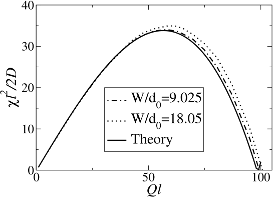
Figure 2: Comparison between the linear stability spectrum of a planar steady-state interface computed with the phase-field model for different interface thicknesses (dot-dashed and dotted lines) and the Mullins-Sekerka theory MS (solid line). Here, $\chi$ is the growth rate of a sinusoidal perturbation of wave number $Q$, and $l=2D/V_{p}$ is the diffusion length. The parameters are for an impure SCN alloy system described in the text with $V_{p}=32$ $\mu$m/sec and $G=140$ K/cm.

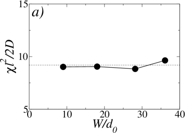
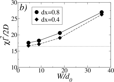
Figure 3: Convergence of the growth rate $\chi(Q)$ as a function of $W/d_{0}$ for: a) $Ql=10.5$, and b) $Ql=87.3$. The dotted lines are the predictions of the Mullins-Sekerka analysis.

We have numerically calculated the stability spectrum of a planar steady-state interface. To this end, the system was initialized with a planar interface at its steady-state position. The concentration in the liquid was set to the exponential steady-state solution of the free boundary problem. A small sinusoidal perturbation of amplitude $A\ll W$ and wave number $Q$ was then applied, and its time evolution was followed by extracting successive interface positions. It follows an exponential increase or decay, and the growth rate $\chi(Q)$ was extracted by a fit of the perturbation amplitude versus time.

In Fig. 2, we compare the results from the numerical simulations to the analytical solution for the Mullins-Sekerka stability spectrum of the free-boundary problem of Eqs. (74)–(76). The convergence is better for smaller wave numbers, which is perfectly reasonable since the ratio of perturbation wavelength to interface thickness scales with $Q$. For $W/d_{0}=9.025$, the phase field model gives a good agreement for almost the whole range of wave numbers, including the maximum, which is the most important part of the spectrum. In Fig. 3, we plot the growth rate $\chi(Q)$ of two selected modes versus the ratio $W/d_{0}$, which shows a fast convergence. For $\Delta x/W=0.4$, the results are fully converged to the theoretical value for $W/d_{0}=4.51$ even for the mode with high wavenumber. It can also be seen that the larger grid spacing of $\Delta x/W=0.8$ introduces slight corrections that are due to the lattice pinning effect (see Ref. KarRap ).

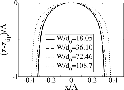
Figure 4: Convergence of the shape of steady-state deep cells as a function of interface thickness. Lengths are scaled by the cell spacing $\Lambda=22.5$ $\mu$m, $V_{p}=32$ $\mu$m/sec and $G=140$ K/cm.

V.2 Cell shapes

To asses the convergence of the models in the nonlinear regime, we have computed shapes of steady-state cells for various values of $W/d_{0}$. The simulation box contains half of a cell, with no-flux boundary conditions along the cell center and the groove. We have considered narrow cells of spacing $\Lambda=1732.8\times d_{0}=22.5$ $\mu$m, since we want to test the convergence of the model for small tip radii; in an extended system, these cells would be unstable to a cell-elimination instability that leads to a doubling of the cell spacing. As initial condition we set $c_{l}=c_{\infty}$, $c_{s}=kc_{l}$ (which, with the definition of Eq. (25) and using $c_{l}^{0}=c_{\infty}/k$, corresponds to $U\equiv-1$ in the whole system), and add a small sinusoidal perturbation to the interface, with a wavelength equal to the cell spacing and its maximum located on the boundary. After a transient where the interface recoils, it reaches steady state in the form of a half cell.

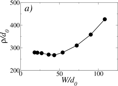
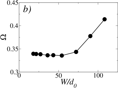
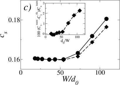
Figure 5: Convergence as a function of interface thickness of various quantities associated with steady-state cell shapes: a) tip radius $\rho$, b) dimensionless tip undercooling $\Omega$ and c) solid concentration in the center of the cell. The diamonds (dashed line) in c) correspond to the values calculated from the Gibbs-Thompson condition using the tip radius of the phase-field shape. The inset shows the relative error of the phase-field results with respect to the Gibbs-Thomson prediction.

The resulting shapes are shown in Fig. 4. For the cell shapes the convergence is faster than for the growth rate, and already simulations with $W/d_{0}\simeq 50$ are well converged. To show more clearly the difference in the speed of convergence, we plot in Fig. 5 the tip radius $\rho/d_{0}$, the tip undercooling $\Omega=1-z_{tip}/l_{T}$ (where $z=0$ corresponds to the position of the steady-state interface), and the solute concentration in the solid in the center of the cell. For the latter, we compare the values that are directly obtained from the simulations (that is, the value of the field $U$ in the center of the cell) to the value expected from the Gibbs-Thomson condition and partition relation at the interface, $c^{th}_{s}=k[k+(1-k)(\Omega-d_{0}/\rho)]$, where the values of $\Omega$ and $\rho$ are obtained from the numerical results (Figs. 5a-b.) Again, all the quantities are well converged for $W/d_{0}\simeq 50$, and even for the ratio $W/d_{0}=72.2$ (corresponding to $\rho/W\simeq 4$), the error in the tip radius for the phase field model is only about 15%, while the equilibrium solute concentration condition at the interface is satisfied within an error of about 1%. The error in this latter condition is small, even for the largest values of $W/d_{0}$ used (Fig. 5c). Since microsegregation is important for metallurgy, the precise calculation of the solute concentration in the solid is an important new feature of the present model.

VI Conclusions and perspectives

We have presented a detailed asymptotic analysis of the phase-field model for alloy solidification that was introduced in Ref. KarmaPRL , and we have simulated directional solidification of a dilute binary alloy. We have found a very good quantitative agreement with the Mullins-Sekerka stability spectrum of a planar interface for typical experimental control parameters. For solidification cells, we found that the solute concentration inside the solid agrees self-consistently with the prediction of the Gibbs-Thomson condition, in contrast to earlier models where the microsegregation was only qualitatively reproduced Warren95 .

This advance relies on a solution of the complete problem of canceling all relevant thin-interface corrections to the original free boundary problem. This opens the way for quantitative comparisons between experiments and simulations both in two and three dimensions, with the concomitant possibility of testing the theories and concepts used to interpret microstructural pattern formation, as was previously done for dendritic solidification.

The present work can be extended along several lines. For example, it has been demonstrated that the concept of the antitrapping current can be generalized to two-phase solidification, which makes it possible to study eutectic or peritectic composite growth with excellent precision Folch03 . Also, the present one-sided model can be combined with a symmetric thermal model to yield a quantitative thermosolutal model of solidification Beckermann . A small solute diffusivity in the solid can also be introduced without appreciable modifications of the present analysis. Finally, the antitrapping current, which was used here to restore the equilibrium partition relation, can also be used to obtain a non-vanishing, specified trapping. This is especially important to extend this model to the whole range of solidification velocity relevant for experiments. In addition, the present model should be applicable to model Hele-Shaw flows when the viscosity of one fluid is much smaller than that of the other.

From a broader perspective, this progress revives the hope of using the phase-field method as an efficient and fully predictive tool for other free boundary and interface growth problems where the dynamics of the two media are not necessarily symmetric, even outside the framework of systems described by a Lyapounov functional. A key element of this progress is the use of non-variational terms which provide additional freedom to obtain the correct mapping between a diffuse interface model and a desired free-boundary problem, such as the antitrapping current here, and other terms in other contexts Folchetal . It is important to emphasize that the interface is spatially diffuse and all interpolation functions are smooth in the present phase-field model. Hence, this model remains simple to implement numerically in comparison to other methods that combine sharp and diffuse interface ingredients Gold ; Amberg .

Let us conclude with a few remarks on the formulation of the model itself. The thermodynamic derivation presented here, which is an alternative to previous expositions of the same model encyclo , establishes new connections to other phase-field models of alloy solidification. As mentioned before, early phase-field models of alloy solidification were plagued by a dependence of the surface tension on the interface thickness that arose from the coupling between the phase-field and concentration equations Wheeler ; Caginalp93 . This problem was solved later by the introduction of two separate concentration fields, one for the solid and one for the liquid, and by interpreting the interface as a mixture of two phases Steinbach98 . The requirement of local equilibrium between the two phases then allows to eliminate one of the concentration fields Kim99 . The resulting model has a surface tension that is independent of the interface thickness and can be used for arbitrary phase diagrams; however, some thin-interface effects remain, in particular surface diffusion Kim99 .

In our derivation, we have succeeded in constructing a quantitative model for an ideal dilute binary alloy with a single concentration field, but two different interpolation functions of the phase field for entropy and internal energy density. This is appealing from a thermodynamic viewpoint, since it maintains the interpretation of the concentration as a local quantity rather than a two-phase mixture. An interesting task would be to generalize this approach to arbitrary phase diagrams and multi-phase solidification.

Appendix A Anomalous interface kinetics

We give here a more detailed discussion of the interface kinetics in a phase-field model without antitrapping current, and with source and diffusion functions given by $h(\phi)=\phi$ and $q(\phi)=(1-\phi)/2$. We will see that in this model, the interface kinetics has logarithmic corrections. This occurs whenever in the limit $\phi\to 1$ the ratio $(h-1)/q$ does not vanish (i.e., remains finite or diverges). Note that, in physical terms, the two functions describe the thermodynamic driving force for solute redistribution during the phase transformation and the diffusivity, respectively. If the latter vanishes faster than the former, the redistribution cannot be completely accomplished on the solid side of the interface, and trapping occurs. We will now analyze this effect in more detail.

Our starting point is Eq. (92) for the first-order diffusion field in the inner region. Without antitrapping current, its solution is

$$U_{1}={\bar{U}}_{1}+\frac{v_{n}}{2}\left[1+(1-k)U_{0}\right]\int_{0}^{\eta}\frac{\phi_{0}(\xi)-1}{q[\phi_{0}(\xi)]}\,d\xi,$$ (134)

which for the above choice of functions becomes

$$U_{1}={\bar{U}}_{1}-v_{n}\left[1+(1-k)U_{0}\right]\eta\,.$$ (135)

This solution, however, is not appropriate since it cannot be matched to the outer solution in the solid, which for a steady state is just a constant. The problem is that we have neglected terms in Eq. (92) that, for this solution, would not be small, which makes the calculation inconsistent. To see this, it is sufficient to remark that both the diffusion term (proportional to $q$) and the redistribution term (proportional to $h-1$) become exponentially small inside the solid. In contrast, for the above solution, the time derivative of $U_{1}$ (equivalent to $v_{n}\partial_{\eta}$ in the moving frame) gives a term of order $\epsilon$ in the equation for $U$, and hence becomes larger than the two mentioned terms far enough in the solid, which violates the counting of orders. In order to get a solution valid everywhere inside the solid, this term has to be included in the equation for $U_{1}$ which becomes

$$\partial_{\eta}[q(\phi_{0})\partial_{\eta}U_{1}]=\frac{v_{n}}{2}\left[1+(1-k)U_{0}\right]\partial_{\eta}\phi_{0}-\epsilon v_{n}\left(\frac{1+k}{2}-\frac{1-k}{2}\phi_{0}\right)\partial_{\eta}U_{1}\,.$$ (136)

By integrating once and using the boundary condition of vanishing current in the solid ($q(\phi_{0})\partial_{\eta}U_{1}\to 0$ for $\eta\to-\infty$), we find

$$q(\phi_{0})\partial_{\eta}U_{1}=\frac{v_{n}}{2}\left[1+(1-k)U_{0}\right](\phi_{0}-1)-\epsilon v_{n}\int_{-\infty}^{\eta}\left(\frac{1+k}{2}-\frac{1-k}{2}\phi_{0}(\xi)\right)\partial_{\xi}U_{1}(\xi)\,d\xi\,.$$ (137)

For the sake of simplicity, let us first discuss the case $k=1$, in which the integral on the right-hand side is simply equal to $U_{1}(\eta)-U_{1}(-\infty)$. It can be seen immediately that this equation admits a solution that has the right limit, $\partial_{\eta}U_{1}\to 0$ for $\eta\to-\infty$. We proceed by constructing an approximate solution by a matching procedure. First, remark that the left-hand side of Eq. (137) is the product of two functions that vanish in the limit $\eta\to-\infty$. Hence, it can be neglected in this limit, and the asymptotic solution is

$$U_{1}(\eta)=U_{1}(-\infty)+\frac{1+(1-k)U_{0}}{2\epsilon}(\phi_{0}-1)\,.$$ (138)

In contrast, in the region of the interface, the newly introduced term, being of order $\epsilon$, is small, which was precisely the reason to neglect it in the usual calculation. Therefore, in this region the solution of Eq. (135) applies. Finally, a matching between the two solutions is found by searching the coordinate $\eta^{\star}$ where their slopes are equal, which, using the fact that $\phi_{0}=-\tanh(\eta/\sqrt{2})$, yields

$$\eta^{\star}=-\sqrt{2}\cosh^{-1}\frac{1}{\sqrt{2\sqrt{2}\epsilon v_{n}}}\,.$$ (139)

In the limit of small velocity $v_{n}$, this simplifies to $\eta^{\star}=(1/\sqrt{2})\ln(\epsilon v_{n}/\sqrt{2})$. It can be checked that, in the matching region, the two terms (diffusion and time derivative) are of similar magnitude, which justifies the matching procedure.

We have hence constructed an approximate solution, which is equal to the one obtained from the standard procedure for $\eta>\eta^{\star}$, and becomes a decaying exponential for $\eta<\eta^{\star}$. Evaluating the solvability integrals with this solution, we find, for example,

$$F^{-}=U_{1}(-\infty)-U_{1}(0)=\frac{v_{n}}{2\sqrt{2}}\left[1+(1-k)U_{0}\right]\left[1-2\ln(\epsilon v_{n}/\sqrt{2})\right]\,.$$ (140)

Similar terms appear also in the integral $K$. Using the identity $\epsilon v_{n}=(W/d_{0})(V_{n}d_{0}/D)=p$, we find that the kinetic coefficient contains, in addition to the usual terms linear in $p$, corrections coming from $\epsilon F^{-}$ that scale as $p\ln p$. This constitutes, for small $p$, a logarithmic correction that makes convergence in $p$ very slow.

This calculation is an approximation, but the conclusion that there are nonlinear correction terms is general, and can be easily interpreted: the anomalous kinetics occurs because solute can escape only from a region of size $\eta^{\star}$ behind the interface, and this size scales logarithmically with $V_{n}$ (and hence $p$) in the limit of small $p$. In this limit, the case of arbitrary $k$ can be easily treated and yields corrections of the form $p\ln(kp)$. In the light of this conclusion, a physical sense can also be given to the condition used in the main body of the paper, namely that the “source function” must decay faster than the diffusivity: under this condition, all solute can escape the advancing interface. Note also that for a more realistic model in which the diffusivity becomes small but finite in the solid, the anomalous dependence of the kinetics on $v_{n}$ stops for $v_{n}<q(+1)$ since then, again, all solute can escape.

Appendix B Discretization

The phase-field and diffusion equations are discretized on a square grid of spacing $\Delta x$. We use standard finite-difference formulas, but a few details are worth mentioning.

For the Laplacian of the phase field, we use the maximally isotropic discretization,

$$\nabla^{2}\phi_{i,j} = \frac{2}{3}(\phi_{i+1,j}+\phi_{i-1,j}+\phi_{i,j+1}+\phi_{i,j-1})$$ (141)

$$+\frac{1}{3}(\phi_{i+1,j+1}+\phi_{i-1,j+1}+\phi_{i+1,j+1}+\phi_{i-1,j-1})-5\phi_{i,j}$$

which avoids the grid corrections to the anisotropy that are discussed in Ref. KarRap .

For the diffusion field $U$, we proceed by first calculating the current in each link, and then summing up all links around a site. On each link, the diffusion part, $j_{u}=-\phi\nabla U$ is calculated with the average of the phase-field according to $j_{u}=-(\phi_{i+1,j}+\phi_{i,j})(u_{i+1,j}-u_{i,j})/(2\Delta x)$ for the $x$ direction, and an analogous expression for the $y$ direction. The most delicate part is the antitrapping current, $j_{at}=a(\phi)W[1+(1-k)U]\hat{n}\partial_{t}\phi$, where $\hat{n}=-\vec{\nabla}\phi/|\vec{\nabla}\phi|$ is the unit normal vector pointing into the liquid. We first evaluate the components of $\vec{\nabla}\phi$. The computation of the component parallel to the link is straightforward. As for the component perpendicular to a link, for a link along the $x$ direction between sites $(i,j)$ and $(i+1,j)$ we use

$$\partial_{y}\phi=\frac{\phi_{i+1,j+1}-\phi_{i+1,j-1}+\phi_{i,j+1}-\phi_{i,j-1}}{4\Delta x},$$ (142)

and similarly for $\partial_{x}\phi$ on links along $y$. From the components of $\vec{\nabla}\phi$, we obtain $\hat{n}$. The product $a(\phi)[1+(1-k)U]\partial_{t}\phi$ is then evaluated at the two end points of the link, and its average value multiplied with the appropriate component of $\hat{n}$ to obtain the current.

References

- (1) L.-Q. Chen, Annu. Rev. Mater. Res. 32, 113 (2002); W. J. Boettinger, J. A. Warren, C. Beckermann, and A. Karma, ibid. 32, 163 (2002).
- (2) M. C. Cross and P. C. Hohenberg, Rev. Mod. Phys. 65, 851 (1993).
- (3) W. Kurz and D. J. Fisher, Fundamentals of Solidification (Trans Tech, Aedermannsdorf, Switzerland, 1992).
- (4) J. Q. Broughton, G. H. Gilmer, and K. A. Jackson, Phys. Rev. Lett. 49, 1496 (1982).
- (5) L. V. Mikheev and A. A. Chernov, J. Cryst. Growth 112, 591 (1991).
- (6) J. J. Hoyt, M. Asta, and A. Karma, Inter. Science 10, 149 (2002).
- (7) A. A. Wheeler, W. J. Boettinger, and G. B. McFadden, Phys. Rev. A45, 7424 (1992); Phys. Rev. E47, 1893 (1993).
- (8) G. Caginalp and W. Xie, Phys. Rev. E48, 1897 (1993).
- (9) A. Karma, in Encyclopedia of Materials: Science and Technology, edited by K. H. J. Buschow, R. W. Cahn, M. C. Flemings, B. Ilschner, E. J. Kramer, S. Mahajan, Volume 7, Elsevier, Oxford, pp. 6873-86 (2001); in Thermodynamics, Microstructures and Plasticity, edited by A. Finel et al., Kluwer Academic Publishers, North Holland, pp. 65-89 (2003).
- (10) J. Tiaden, B. Nestler, H.-J. Diepers, and I. Steinbach, Physica D 115, 73 (1998).
- (11) S. G. Kim, W. T. Kim, and T. Suzuki, Phys. Rev. E 60, 7186 (1999).
- (12) J. Bragard, A. Karma, Y. H. Lee, M. Plapp, Interface Science 10, 121 (2002).
- (13) A. Karma and W.-J. Rappel, Phys. Rev. E 53, R3017 (1996); Phys. Rev. E 57, 4323 (1998).
- (14) N. Provatas, N. Goldenfeld, and J. Dantzig, Phys. Rev. Lett. 80, 3308 (1998); J. Comp. Phys. 148, 265 (1999).
- (15) M. Plapp and A. Karma, Phys. Rev. Lett. 84, 1740 (2000); J. Comp. Phys. 165, 592 (2000).
- (16) A. Karma, Y. H. Lee, and M. Plapp, Phys. Rev. E61 3996 (1999).
- (17) J. A. Warren and W. J. Boettinger, Acta Metall. Mater. 43, 689 (1995).
- (18) R. F. Almgren, SIAM J. Appl. Math 59, 2086 (1999).
- (19) A. Karma, Phys. Rev. Lett. 87, 115701 (2001).
- (20) W. Kurz and D. J. Fisher, Fundamentals of solidification (Trans Tech, Aedermannsdorf, Switzerland, 1992).
- (21) M. J. Aziz, J. Appl. Phys. 53, 1158 (1982); N. A. Ahmad, A. A. Wheeler, W. J. Boettinger, and G. B. McFadden, Phys. Rev. E 58, 3436 (1998).
- (22) K. R. Elder, M. Grant, N. Provatas, and J. M. Kosterlitz, Phys. Rev. E 64, 021604 (2001).
- (23) G. B. McFadden, A. A. Wheeler, and D. M. Anderson, Physica D 144, 154 (2000).
- (24) W. W. Mullins and R. F. Sekerka, J. Appl. Phys. 35, 444 (1964).
- (25) S-L. Wang, R.F. Sekerka, A.A. Wheeler, B.T. Murray, S.R. Coriell, R.J. Braun, and G.B. McFadden, Physica D 69, 189 (1993).
- (26) R. Folch, J. Casademunt, A. Hernández-Machado, and L. Ramírez-Piscina, Phys. Rev. E 60, 1724 (1999); 60, 1734 (1999).
- (27) M. Georgelin and A. Pocheau, Phys. Rev. E 57, 3189 (1998); Eur. Phys. J B 4, 169 (1998).
- (28) R. Folch and M. Plapp, Phys. Rev. E 68, 010602R (2003).
- (29) J. C. Ramirez, C. Beckermann, A. Karma, and H.-J. Diepers, Phys. Rev. E 69, 051607 (2004).
- (30) Y.-T. Kim, N. Goldenfeld, and J. Dantzig, Phys. Rev. E 62, 2471 (2000).
- (31) G. Amberg, Phys. Rev. Lett. 91, 265505 (2003).