Electrostatic Contribution to the Persistence Length of a Semiflexible Dipolar Chain

Abstract

We investigate the electrostatic contribution to the persistence length of a semiflexible polymer chain whose segments interact via a screened Debye-Hückel dipolar interaction potential. We derive the expressions for the renormalized persistence length on the level of a $1/D$-expansion method already successfully used in other contexts of polyelectrolye physics. We investigate different limiting forms of the renormalized persistence length of the dipolar chain and show that in general it depends less strongly on the screening length than in the context of a monopolar chain. We show that for a dipolar chain the electrostatic persistence length in the same regime of the parameter phase space as the original Odijk-Skolnick-Fixman (OSF ) form for a monopolar chain depends logarithmically on the screening length rather than quadratically. This can be understood solely on the basis of a swifter decay of the dipolar interactions with separation compared to the monopolar electrostatic interactions. We comment also on the general contribution of higher multipoles to the electrostatic renormalization of the bending rigidity.

1 Introduction

Semiflexible polyelectrolytes are ubiquitous in biological context ranging from biopolymers such as DNA, filamentous $F$ actin, microtubules, and then all the way to molecular aggregates such as micelles or even whole organisms as in bacterial $fd$ viruses or the tobacco mosaic virus. In all these cases we are dealing with objects that at an appropriate scale behave as Euler-Kirchhoffian elastic filaments. The most important mechanical characteristics in these molecular systems is the persistence length stemming from the bending rigidity of the polymer that can exhibit enormous variation in magnitude bracketted by nm on the lower end and mm on the upper end.

The bending rigidity and thus the persistence length is a consequence of short range atomic and molecular interactions and is itself a mesoscopic property [1]. For charged semiflexible polymers the long range nature of the electrostatic interactions modifies the value of the persistence length as is well known from the seminal work of Odijk, Skolnick and Fixman (OSF) [2]. Recent detailed critical assessment of the OSF conjecture [3, 4, 5] confirmed the universality of the dependence of the persistence length on the parameters of the electrostatic interaction. It appears that the OSF behavior characterized by the inverse dependence of the persistence length on the ionic strength of the bathing medium is quite robust. One of the main ingredients of the OSF ideology is a complete lack of any atomic or molecular specificity in the interaction between charge segments along the polyelectrolyte. By assumption the mobile charges in solution and the fixed charges on the polyelectrolyte backbone interact only via generic (screened) Coulomb interaction. Though this assumption seems to be reasonable it would be appropriate to investigate what kind of behavior of persistence length is conferred by the effects of strong specificity as in e.g. the case of specific ion adsorption. Recent experiments also suggest that reevaluation of the basic assumptions in our understanding of counterion - backbone interactions in polyelectrolytes would be highly desirable [6].

In specific ion adsorption mobile charges from the bathing solution and fixed charges along the polyelectrolyte can combine, leading to the emergence of higher multipoles along the polyelectrolyte chain, the first one being a dipole stemming from the association of a negative fixed charge and a specifically adsorbed mobile positive charge from the bathing solution. The same situation though for different reasons, specifically due to the low dielectric constant envoronment, could be obtained also in the context of ionomers [7]. Similar consideration could apply also to electrorheological or ferrofluids in external fields.

Muthukumar [8] was the first to realize the importance and the extent of modifications wrought by the first higher multipole i.e. the dipole, on the behavior of a flexible polyelectrolyte described on the level of the Edwards Hamiltonian. He discovered the formation of localized aggregated structures along the chain that dominate the statistical behavior of the flexible polyelectrolyte chain. They are characterized by a different scaling of the size of the chain with respect to its length and depend continuously on the parameters of the dipolar interaction potential.

Chain flexibility as formalized by the Edwards Hamiltonian [9] is essential for emergence of this type of aggregated structures. Now assume a dipolar semiflexible chain, described as an Euler-Kirchhoffian filament with dipolar intersegment interactions. On top of that assume that the length of the chain is the largest length in the problem. This constitutes a complementary limit to be contrasted with the Muthukumar calculation. The analysis provided by Muthukumar and the one detailed below should thus brackett the behavior of any real polyelectrolyte chain with dipolar charges along its length.

The problem with dipolar interactions is that they depend on the local orientation of the polyelectrolyte segments. This complicates the evaluation of the partition function of the semiflexible chain in an essentail manner. In order to make this complicated problem tractable, we will invoke the $1/D$-expansion method [11] that has already been successfully applied to the problem of persistence length renormalization of a semiflexible polyelectrolyte chain [12] with monopolar charges. This will allow us to explicitly evaluate the electrostatic contribution to the persistence length of a dipolar chain. As a point of departure we will assume that the dipolar charges along the chain interact via a screened Coulombic interaction potential, the range of which is characterized by the Debye screening length [13]. We will derive the complete dependence of the electrostatic persistence length on the parameters of the dipolar interaction potential and show that it leads to a different behavior regarding its dependence on the ionic strength of the bathing solution then the standard OSF result. We find basically two different regimes for the bahavior of the electrostatic persistence length of a dipolar chain

• for small but non-vanishing values of the screening length $\lambda_{D}$ the electrostatic contribution to the persistence length behaves as

  $$L_{P}^{(R)}=L_{P}^{(0)}+const.\log{\lambda_{D}}$$

  where $L_{P}^{(0)}$ is the bare value of the persistence length. This expression would superseed the OSF $\lambda_{D}^{2}$ result valid for monopolar interactions. Obviously the dipolar electrostatic renormalization of the persistence length depends more gently on the screening length.

• for large values of the screening length $\lambda_{D}$ the electrostatic contribution to the persistence length behaves as

  $$L_{P}^{(R)}=const.{\lambda_{D}}^{\beta},$$

  where $\beta$ equals either $3/4$ or $3$, depending on the strength of the dipolar interaction. This result should be compared with various variational estimates of a sub-OSF behavior for a monopolar chain that lead to $\beta$ in the vicinity of $1$.

These two regimes stemm from two different limiting forms of a single equation giving the renormallized value of the persistence length as a function of the parameters describing the dipolar interactins along the chain. We also present complete numerical solutions of this equation in various regions of the parameter space.

The outline of the paper is as follows. In Section 1 we first rewrite the Hamiltonian of a semiflexible polymer chain with screened dipolar interactions, assumed to be composed of the Euler-Kirchhoff elastic energy and the interaction energy, in a form that allows for a straightforward application of the $1/D$-expansion ansatz. We assume that the dipoles of the polymer segments are oriented along the local tangent vectors of the chain. This effective Hamiltonian captures the elasticity of the chain, the inextensibility of the chain and the fact that electrostatic interactions depend on the position of the interacting segments as well as their orientation. Section 2 introduces all the important approximations in order to make the evaluation of the partition function of the chain tractable. A diagonalization ansatz is introduced for the orientational part of the Hamiltonian, a global inextensibility constraint is substituted for the local one and a saddle point evaluation is introduced for all the auxiliary fields that do not enter the Hamiltonian on a quadratic level. In section 3 the saddle point equations are solved explicitly by expanding all the Fourier components of different auxiliary fields to the fourth order. This is consistent with the semiflexible ansatz for the configuraional part of the Hamiltonian of the chain. Section 4 introduces explicit equations for the bending rigidity renormalization that follow from the saddle point equations of the previous section. These equations are solved numerically in the last section. Different limiting forms of the numeric solutions for limited regions of the parameter phase space are derived also analytically. We take a critical look at the results derived in this work and comment on the implied limitations of their validity and their connection with previous work on the electrostatic renormalization of the rigidity of semiflexible polymers.

2 The effective Hamiltonian

We investigate a semiflexible polymer chain with dipolar charges along the chain. The dipoles can be either structural or they can be a consequence of the specific adsorption of e.g. positive mobile charges from the bathing solution onto the fixed negative charges on the polyelectrolyte backbone. The total interaction energy of the chain is given by

$$\frac{1}{2}\int_{0}^{L}\!\!\!\int_{0}^{L}V({\bf r}(s),{\bf r}(s^{\prime}))dsds^{\prime}$$ (1)

where

$$V({\bf r}(s),{\bf r}(s^{\prime})) = \frac{e^{-\kappa|{\bf r}(s)-{\bf r}(s^{\prime})|}}{4\pi\epsilon\epsilon_{0}|{\bf r}(s)-{\bf r}(s^{\prime})|^{5}}\left(|{\bf r}(s)-{\bf r}(s^{\prime})|^{2}(1+\kappa|{\bf r}(s)-{\bf r}(s^{\prime})|)\mathbf{p}(s)\cdot\mathbf{p}(s^{\prime})-\right.$$ (2)

$$\left.-(3+3\kappa|{\bf r}(s)-{\bf r}(s^{\prime})|+(\kappa|{\bf r}(s)-{\bf r}(s^{\prime})|)^{2})(\mathbf{p}(s)\cdot({\bf r}(s)-{\bf r}(s^{\prime})))(\mathbf{p}(s^{\prime})\cdot({\bf r}(s)-{\bf r}(s^{\prime})))\right),$$

with $|{\bf r}(s)-{\bf r}(s^{\prime})|$ the separation between two segments located at ${\bf r}(s)$ and ${\bf r}(s^{\prime})$ along the chain, $s$ is the arclength of the chain, and $\mathbf{p}(s)$ and $\mathbf{p}(s^{\prime})$ are dipoles per unit length located at $s$ and $s^{\prime}$. The above form of the screened dipolar interaction follows straightforwardly from the second order multipole expansion of the screened Coulomb kernel [14] and reduces to the usual form of the dipolar interaction in the lim it of no screening. On the Debye - Hückel level $\kappa=\lambda_{D}^{-1}$ where $\lambda_{D}$ is the Debye screening length. We furthermore assume that the dipole per unit length along the chain is given by

$${\bf p}(s)=p_{0}\partial_{s}{\bf r}(s)$$ (3)

where $p_{0}$ is the strength of the dipolar moment per unit length of the segment and $\partial_{s}{\bf r}(s)=\dot{\bf r}(s)$ is the unit tangent vector. It is thus assumed that the dipoles point along the chain, and that the component of the dipoles perpendicular to the local axis of the chain is averaged out to zero. Or model is thus ”perpendicular” to ther case investigated in the context of protein folding [15]. The interactions along the chain are therefore described with a generic form of segment - segment interactions that can be cast into the form

$$V({\bf r}(s),{\bf r}(s^{\prime})) = V_{R}({\bf r}(s)-{\bf r}(s^{\prime}))\partial_{s}{\bf r}(s)\partial_{s^{\prime}}{\bf r}(s^{\prime})-$$

$$-V_{P}({\bf r}(s)-{\bf r}(s^{\prime}))\left(\partial_{s}{\bf r}(s)\cdot({\bf r}(s)-{\bf r}(s^{\prime}))\right)\left(\partial_{s^{\prime}}{\bf r}(s^{\prime})\cdot({\bf r}(s)-{\bf r}(s^{\prime}))\right),$$

(4)

with

$$V_{R}({\bf r}(s)-{\bf r}(s^{\prime})) = v_{0}\frac{e^{-\kappa|{\bf r}(s)-{\bf r}(s^{\prime})|}}{|{\bf r}(s)-{\bf r}(s^{\prime})|^{3}}\left(1+\kappa|{\bf r}(s)-{\bf r}(s^{\prime})|\right),$$

$$V_{P}({\bf r}(s)-{\bf r}(s^{\prime})) = v_{0}\frac{e^{-\kappa|{\bf r}(s)-{\bf r}(s^{\prime})|}}{|{\bf r}(s)-{\bf r}(s^{\prime})|^{5}}\left(3+3\kappa|{\bf r}(s)-{\bf r}(s^{\prime})|+\kappa^{2}|{\bf r}(s)-{\bf r}(s^{\prime})|^{2}\right),$$ (5)

Obiosuly the interaction Eq. 4 depends on the positions of the interacting segments as well as on their orientation. This is the fundamental difference between monopolar and dipolar interactions. We have defined

$$v_{0}=\frac{p_{0}^{2}}{4\pi\epsilon\epsilon_{0}}=k_{B}T~{}~{}\ell_{B}\left(\frac{p_{0}^{2}}{e_{0}^{2}}\right),$$ (6)

where $\ell_{B}$ is the Bjerrum length [13]. The units of $v_{0}$ are energy times length and are thus the same as the units of bending modulus of a semiflexible polymer chain.

The generic form of the interaction Eq. 4 together with the Euler-Kirchhoffian elastic conformational part of the mesoscopic free energy [16] can now be used to investigate the statistical behavior of a semiflexible dipolar chain. The mesoscopic Hamiltonian of the chain can be written canonically as

$${\cal H}[{\bf r}(s)]=\frac{1}{2}K_{C}\int_{0}^{L}ds\left(\partial^{2}_{s}{\bf r}(s)\right)^{2}+\frac{1}{2}\int_{0}^{L}\!\!\!\int_{0}^{L}dsds^{\prime}V({\bf r}(s),{\bf r}(s^{\prime})).$$ (7)

where the local curvature is

$$\partial^{2}_{s}{\bf r}(s)=\frac{\partial^{2}{\bf r}(s)}{\partial s^{2}}.$$ (8)

The bending rigidity $K_{C}$ is connected with the bare persistence length via $K_{C}=k_{B}T~{}L_{P}^{{(0)}}$. Since in what follows the chain is assumed to be inextensible an additional constraint of $\partial_{s}{\bf r}(s)\partial_{s}{\bf r}(s)=1$ should be taken into account. The partition function thus assumes the form

$$\Xi=\int{\cal D}[{\bf r}(s)]\Pi_{s}\delta^{3}\left((\partial_{s}{\bf r}(s))^{2}-1\right)~{}\exp{-\beta{\cal H}[{\bf r}(s)]}.$$ (9)

There are two difficult problems connected with this partition function: first of all we have the constraint of inextensibility that has to be enforced locally for every conformation of the chain, and on top of this there is the non-locality of the segment-segment interaction potential that couples different segments along the chain and depends also on their orientation. We will address both problems systematically by applying the method of Lagrange multipliers [12].

To this effect we will introduce two additional terms into the interaction Hamiltonian. The inextensibility constraint is dealt with via the Lagrange multiplier $\lambda(s)$, leading to an additional term in the Hamiltonian of the form

$$\delta{\cal H}_{1}=\frac{1}{2}\int ds\lambda(s)\left((\partial_{s}{\bf r}(s))^{2}-1\right),$$ (10)

together with an additional trace over $\lambda(s)$ in the expression for the partition function. In what follows we will assume that the inextensiblity constraint can be implemented globally instead of locally [17]. This automatically means that $\lambda(s)=\lambda$. The non-locality of the interaction potential is more difficult to deal with then in the case of a chain without orientationally dependent interactions. In order to pave the way for an approximate evaluation of the partition function we introduce two new Lagrange multipliers in the form of two tensorial auxiliary fields. First of all we define

$${\cal B}_{ik}(s,s^{\prime})=\left({\bf r}_{i}(s)-{\bf r}_{i}(s^{\prime})\right)\left({\bf r}_{k}(s)-{\bf r}_{k}(s^{\prime})\right)$$ (11)

and then

$${\cal T}_{ik}(s,s^{\prime})=\partial_{s}{\bf r}_{i}(s)\partial_{s}{\bf r}_{k}(s).$$ (12)

We notice immediately these two fundamental identities

$${\rm Tr}~{}{\cal B}_{ik}(s,s^{\prime})=\left({\bf r}(s)-{\bf r}(s^{\prime})\right)^{2}\quad{\rm and}\quad{\rm Tr}~{}{\cal T}_{ik}(s,s^{\prime})=\partial_{s}{\bf r}(s)\cdot\partial_{s}{\bf r}_{(}s).$$ (13)

We thus conclude that ${\rm Tr}~{}{\cal B}_{ik}(s,s^{\prime})$ is equivalent to ${\cal B}(s,s^{\prime})$ introduced in the context of orientationaly independent intrachain interactions [12]. Introducing furthermore the following two additional coupling terms

$$\delta{\cal H}_{2} = \frac{1}{2}\int\!\!\int dsds^{\prime}g_{ik}(s,s^{\prime})\left(\left({\bf r}_{i}(s)-{\bf r}_{i}(s^{\prime})\right)\left({\bf r}_{k}(s)-{\bf r}_{k}(s^{\prime})\right)-{\cal B}_{ik}(s,s^{\prime})\right)$$

$$\delta{\cal H}_{3} = \frac{1}{2}\int\!\!\int dsds^{\prime}p_{ik}(s,s^{\prime})\left(\partial_{s}{\bf r}_{i}(s)\partial_{s}{\bf r}_{k}(s)-{\cal T}_{ik}(s,s^{\prime})\right).$$ (14)

we can write the partition function in the following form

$$\Xi=\int{\cal D}[{\bf r}(s)]{\cal D}[\lambda(s)]{\cal D}[g_{ik}(s)]{\cal D}[{\cal B}_{ik}(s)]{\cal D}[p_{ik}(s)]{\cal D}[{\cal T}_{ik}(s)]~{}\exp{-\beta\overline{\cal H}[{\bf r}(s)]},$$ (15)

where the effective Hamiltonian $\overline{\cal H}[{\bf r}(s)]$ is given by

$$\overline{\cal H}[{\bf r}(s)]={\cal H}[{\bf r}(s)]+\delta{\cal H}_{1}[{\bf r}(s)]+\delta{\cal H}_{2}[{\bf r}(s)]+\delta{\cal H}_{3}[{\bf r}(s)].$$ (16)

The new auxiliary fields $g_{ik}(s,s^{\prime})$ and $p_{ik}(s,s^{\prime})$ thus act as tensorial Lagrange multipliers setting the constraints $\left({\bf r}_{i}(s)-{\bf r}_{i}(s^{\prime})\right)\left({\bf r}_{k}(s)-{\bf r}_{k}(s^{\prime})\right)-{\cal B}_{ik}(s,s^{\prime})=0$ and $\partial_{s}{\bf r}_{i}(s)\partial_{s}{\bf r}_{k}(s)-{\cal T}_{ik}(s,s^{\prime})=0$. In the new variable space the segment-segment interaction potential can be obtained in a more transparent form as

$$V({\bf r}(s),{\bf r}(s^{\prime})) = V_{R}({\rm Tr}~{}{\cal B}_{ik}(s,s^{\prime})){\rm Tr}~{}{\cal T}_{ik}(s,s^{\prime})-$$ (17)

$$-V_{P}({\rm Tr}~{}{\cal B}_{ik}(s,s^{\prime})){\cal B}_{ik}(s,s^{\prime}){\cal T}_{ik}(s,s^{\prime})=V\left({\cal B}_{ik}(s,s^{\prime}),{\cal T}_{ik}(s,s^{\prime})\right).$$

In order to arrive at a more transparetn form of the partition function we furthermore introduce the following two new variables

$$\lambda^{(c)}_{ik}(s,s^{\prime}) = \lambda~{}\delta_{ik}\delta(s-s^{\prime})+p_{ik}(s,s^{\prime})$$

$$g^{(c)}_{ik}(s,s^{\prime}) = \frac{1}{2}\delta(s-s^{\prime})\int ds"\left(g_{ik}(s,s")+g_{ik}(s",s^{\prime})\right)-g_{ik}(s,s^{\prime}).$$ (18)

With these new definitions the effective Hamiltonian can be finally reduced to this fairly complicated form

$$\overline{\cal H}[{\bf r}(s)] = \frac{1}{2}K_{C}\int ds(\partial^{2}_{s}{\bf r}(s))^{2}-\textstyle{\frac{1}{2}}\lambda\int ds+$$ (19)

$$+\frac{1}{2}\int\int dsds^{\prime}\lambda^{(c)}_{ik}(s,s^{\prime})\partial_{s}{\bf r}_{i}(s)\partial_{s}{\bf r}_{k}(s)+\frac{1}{2}\int\int dsds^{\prime}2g^{(c)}_{ik}(s,s^{\prime}){\bf r}_{i}(s){\bf r}_{k}(s)-$$

$$-\frac{1}{2}\int\int dsds^{\prime}g_{ik}(s,s^{\prime}){\cal B}_{ik}(s,s^{\prime})-\frac{1}{2}\int\int dsds^{\prime}p_{ik}(s,s^{\prime}){\cal T}_{ik}(s,s^{\prime})+$$

$$+\frac{1}{2}\int\int dsds^{\prime}V\left({\cal B}_{ik}(s,s^{\prime}),{\cal T}_{ik}(s,s^{\prime})\right).$$

The above form of the Hamiltonian together with Eq. 15 represents at this stage an exact expression for the partition function. This is the starting point of different approximations introduced below.

Though the above form of the effective Hamiltonian looks prohibitively complicated it can in fact be reduced to analytical quadratures provided one devises a powerfull enough approximation scheme. It was shown in recent work [12, 18, 19] that the $1/D$-expansion method, where $D$ here and below is the dimensionality of the embedding space, can be fruitfully applied to polymer problems of the above type and we will use our experience gained in the context of monopolar interactions [12] to tackle also the more complicated case of multipolar interactions as implied by the Hamiltonian Eq. 19.

3 The ansatz

Our rationale for writing the effective Hamiltonian in the form Eq. 19 is that it will be shown to be amenable to straightforward approximations leading to a closed form evaluation of the partition function. Similar methods have been already used successfully in the context of monopolar interactions. First of all we will introduce a diagonalization ansatz of the form

$$g_{ik}(s,s^{\prime}) = g(s,s^{\prime})\delta_{ik}$$

$$p_{ik}(s,s^{\prime}) = p(s,s^{\prime})\delta_{ik}.$$ (20)

Though this ansatz is not absolutely necessary in order to make progress in the evaluation of the partition function Eq. 15, it certainly makes the whole calculation manageable and controllable, reducing its overall complexity to a bare minimum. The above ansatz clearly implies also

$$g^{(c)}_{ik}(s,s^{\prime}) = g^{(c)}(s,s^{\prime})\delta_{ik}$$

$$\lambda^{(c)}_{ik}(s,s^{\prime}) = \lambda^{(c)}(s,s^{\prime})\delta_{ik}.$$ (21)

In order to be consistent we must also introduce the same type of diagonalization ansatz for the fields ${\cal B}_{ik}(s,s^{\prime})$ and ${\cal T}_{ik}(s,s^{\prime})$, which are conjugate to the fields $g_{ik}(s,s^{\prime})$ and $p_{ik}(s,s^{\prime})$. We formulate this as

$${\cal B}_{ik}(s,s^{\prime}) = \textstyle{\frac{1}{D}}{\cal B}(s,s^{\prime})\delta_{ik}$$

$${\cal T}_{ik}(s,s^{\prime}) = \textstyle{\frac{1}{D}}{\cal T}(s,s^{\prime})\delta_{ik}.$$ (22)

In this way we can write ${\rm Tr}~{}{\cal B}_{ik}(s,s^{\prime})={\cal B}(s,s^{\prime})$ and ${\rm Tr}~{}{\cal T}_{ik}(s,s^{\prime})={\cal T}(s,s^{\prime})$. Since we are not concerned here with explicit analysis of finite size effects we can assume overall that the $(s,s^{\prime})$ dependencies actually reduce to $(s-s^{\prime})$. Similarly to the case of orientationally independent intrachain interactions we see that the partition function is now quadratic in ${\bf r}(s)$ and its first and second derivatives. We can thus trace over these harmonic degrees of freedom [12]. Expanding the whole effective Hamiltonian around a reference configuration ${\bf r}_{0}(s)$ and introducing the Fourier components of different fields in the standard way we obtain after tracing out the harmonic degrees of freedom the following form of the effective Hamiltonian

$$\overline{\cal H}^{\prime} = \overline{\cal H}[{\bf r}_{0}(s)]+\textstyle{\frac{Dk_{B}T~{}}{2}}\sum_{Q}\log{{\cal G}(Q)}-\frac{1}{2}\lambda\int ds+$$ (23)

$$-\frac{1}{2}\int\int dsds^{\prime}g(s,s^{\prime}){\cal B}(s,s^{\prime})-\frac{1}{2}\int\int dsds^{\prime}p(s,s^{\prime}){\cal T}(s,s^{\prime})+$$

$$+\frac{1}{2}\int\int dsds^{\prime}V\left({\cal B}(s,s^{\prime}),{\cal T}(s,s^{\prime})\right),$$

where the self energy function ${\cal G}(Q)$ is given by

$${\cal G}(Q)=\left(K_{C}Q^{4}+\lambda^{(c)}(Q)Q^{2}+2g^{(c)}(Q)\right).$$ (24)

Here $\lambda^{(c)}(Q)$ and $g^{(c)}(Q)$ are of course the Fourier components of the fields $g^{(c)}(s-s^{\prime})$ and $\lambda^{(c)}(s-s^{\prime})$. The Hamiltonian of the reference configuration ${\bf r}_{0}(s)$ can be derived as

$$\overline{\cal H}[{\bf r}_{0}(s)] = \frac{1}{2}K_{C}\int ds(\partial^{2}_{s}{\bf r}_{0}(s))^{2}+\frac{1}{2}\int\!\!\!\int dsds^{\prime}\lambda^{(c)}(s-s^{\prime})\left(\partial_{s}{\bf r}_{0}(s)\cdot\partial_{s}{\bf r}_{0}(s)\right)+$$ (25)

$$+\frac{1}{2}\int\!\!\!\int dsds^{\prime}2g^{(c)}(s-s^{\prime})\left({\bf r}_{0}(s)\cdot{\bf r}_{0}(s)\right).$$

All along we disregard the finite (chain) size effects and assume that the chain is homogeneous and $s,s^{\prime}$ dependence is actually equivalent to $|s-s^{\prime}|$ dependence. This assumption furthermore implies that the length of the chain is the largest length in the problem. Thus with this line of reasoning

$$g^{(c)}(Q) = \int du\cos{Qu}~{}g^{(c)}(u)=g(Q)-g(Q=0)$$

$$\lambda^{(c)}(Q) = \int du\cos{Qu}~{}\lambda^{(c)}(u).$$ (26)

From here we can also straightforwardly conclude that we have the following identities for the functional derivatives

$$\frac{\delta g^{(c)}(Q)}{\delta g(s,s^{\prime})} = 1-\cos{Q(s-s^{\prime})}$$

$$\frac{\delta\lambda^{(c)}(Q)}{\delta\lambda(s,s^{\prime})} = \cos{Q(s-s^{\prime})}.$$ (27)

The next logical step in order to evaluate the partition function Eq. 15 would be to trace out the auxiliary fields $\lambda(s),g_{ik}(s),{\cal B}_{ik}(s),p_{ik}(s),{\cal T}_{ik}(s)$. Unfortunately these fields enter the effective Hamiltonian non-linearly and they can not be simply traced over. Thus we have to introduce a new approximation at this point: instead of integrating over the auxiliary fields we will simply evaluate the saddle - point of $\overline{\cal H}^{\prime}$ with respect to these fields. This is easier and most importantly it is feasible to do. It is thus at this juncture that a critical step in the derivation of the partition function has to be made that constitutes the essence of the $1/D$-expansion method as applied to the polymer problem. The details and ramifications of this step have been addressed in the previous work [12].

4 The saddle point equations

The saddle point of the effective Hamiltonian Eq. 23 w.r.t. the fields $\lambda(s,s^{\prime})$, ${\cal B}(s,s^{\prime})$, $g(s,s^{\prime})$, ${\cal T}(s,s^{\prime})$ and $p(s,s^{\prime})$ can be obtained straightforwardly in a standard fashion. For the saddle point in the $\lambda(s,s^{\prime})$ variable we obtain the following relation

$$1=\left(\partial_{s}{\bf r}_{0}(s)\cdot\partial_{s}{\bf r}_{0}(s)\right)+Dk_{B}T~{}\sum_{Q}{\cal G}^{-1}(Q)Q^{2},$$ (28)

The next saddle point that we evaluate is ${\cal B}(s,s^{\prime})$. It leads to the following equation

$$g^{(c)}(Q)=\int ds(1-\cos{Qs})\frac{\partial V({\cal B}(s),{\cal T}(s))}{\partial{\cal B}(s)}.$$ (29)

Then follows the saddle point in $g(s,s^{\prime})$, giving rise to

$${\cal B}(s,s^{\prime})=\left({\bf r}_{0}(s)-{\bf r}_{0}(s^{\prime})\right)^{2}+2Dk_{B}T~{}\sum_{Q}{\cal G}^{-1}(Q)(1-\cos{Q(s-s^{\prime})}).$$ (30)

Furthermore the saddle point in the variable ${\cal T}(s,s^{\prime})$ leads to

$$p(Q)=\int ds\cos{Qs}\frac{\partial V({\cal B}(s),{\cal T}(s))}{\partial{\cal T}(s)},$$ (31)

and finally the saddle point in $p(s,s^{\prime})$ gives rise to

$${\cal T}(s,s^{\prime})=\left(\partial_{s}{\bf r}_{0}(s)\cdot\partial_{s}{\bf r}_{0}(s)\right)+Dk_{B}T~{}\sum_{Q}{\cal G}^{-1}(Q)Q^{2}\cos{Q(s-s^{\prime})}.$$ (32)

We now assume that we can retain only terms up to the fourth order in $Q$ for the functions $\lambda^{(c)}(Q)$ and $g^{(c)}(Q)$. This is consistent with the fact that the original non-interaction part of the Hamiltonian contains only Euler-Kirchhoffian elasticity and is thus at most of fourth order in the $Q$ space. In this way we obtain the following expansion

$$\lambda^{(c)}(Q)=\lambda+p(Q)=\lambda+\int ds\frac{\partial V({\cal B}(s),{\cal T}(s))}{\partial{\cal T}(s)}-\frac{Q^{2}}{2}\int dss^{2}\frac{\partial V({\cal B}(s),{\cal T}(s))}{\partial{\cal T}(s)}+\dots,$$ (33)

as well as

$$2g^{(c)}(Q)=Q^{2}\int dss^{2}\frac{\partial V({\cal B}(s),{\cal T}(s))}{\partial{\cal B}(s)}-\frac{Q^{4}}{12}\int dss^{4}\frac{\partial V({\cal B}(s),{\cal T}(s))}{\partial{\cal B}(s)}+\dots.$$ (34)

Thus we have basically derived an expansion also for the self-energy Eq. 24 which can now be cast into the form

$${\cal G}(Q)=\left(\lambda+\delta\lambda\right)Q^{2}+\left(K_{C}+\delta K_{C}\right)Q^{4}+\dots=\lambda^{(R)}Q^{2}+K^{(R)}_{C}Q^{4}+\dots.$$ (35)

The expansion in $Q$ to the fourth order thus allows us to introduce the renormalized values of the parameters $\lambda$ and $K_{C}$ via

$$\lambda^{(R)}=\lambda+\delta\lambda\qquad K^{(R)}_{C}=K_{C}+\delta K_{C},$$ (36)

where we introduced the following two abbreviations

$$\delta\lambda = \int ds\frac{\partial V({\cal B}(s),{\cal T}(s))}{\partial{\cal T}(s)}+\int ds~{}s^{2}\frac{\partial V({\cal B}(s),{\cal T}(s))}{\partial{\cal B}(s)}$$

$$\delta K_{C} = -\textstyle{\frac{1}{2}}\int ds~{}s^{2}\frac{\partial V({\cal B}(s),{\cal T}(s))}{\partial{\cal T}(s)}-\textstyle{\frac{1}{12}}\int ds~{}s^{4}\frac{\partial V({\cal B}(s),{\cal T}(s))}{\partial{\cal B}(s)}.$$ (37)

At this point we are in a position to evaluate all the $Q$ integrals in the saddle point equations. Thus instead of Eqs. 28, 30 and 32 we remain with

$$1 = \left(\partial_{s}{\bf r}_{0}(s)\cdot\partial_{s}{\bf r}_{0}(s)\right)+\frac{Dk_{B}T~{}}{4\sqrt{\lambda^{(R)}K^{(R)}_{C}}},$$

$${\cal B}(s,s^{\prime}) = \left({\bf r}_{0}(s)-{\bf r}_{0}(s^{\prime})\right)^{2}+\frac{Dk_{B}T~{}}{2\lambda^{(R)}}\left((s-s^{\prime})+\sqrt{\frac{K^{(R)}_{C}}{\lambda^{(R)}}}(e^{-\sqrt{\frac{\lambda^{(R)}}{K^{(R)}_{C}}}(s-s^{\prime})}-1)\right)$$

$${\cal T}(s,s^{\prime}) = \left(\partial_{s}{\bf r}_{0}(s)\cdot\partial_{s}{\bf r}_{0}(s)\right)+\frac{Dk_{B}T~{}}{4\sqrt{\lambda^{(R)}K^{(R)}_{C}}}e^{-\sqrt{\frac{\lambda^{(R)}}{K^{(R)}_{C}}}(s-s^{\prime})}.$$ (38)

Finally we have to address the question of the reference state. Assuming with sufficient generality that the reference configuration of the chain is a straight line, thus ${\bf r}_{0}(s)=\zeta s{\bf e}$, where ${\bf e}$ is a constant vector [12]. At this point we can investigate also the saddle point of $\overline{\cal H}[{\bf r}_{0}(s)]$ with respect to $\zeta$, the new variable, which reduces to the following two equations

$$\frac{\partial{\cal G}(Q)}{\partial Q^{2}}=0\quad{\rm or}\quad\zeta=0.$$ (39)

On general grounds $\zeta$ can be non-zero only at zero temperature, when there are no fluctuations and the chain can indeed exhibit straight configurations. For any finite temperature straight configurations are not feasible without external constraints and we should rather have $\zeta=0$. Taking this into account and solving the first of the above equations i.e. we obtain

$$1=\frac{dk_{B}T~{}}{4\sqrt{\lambda^{(R)}K^{(R)}_{C}}}$$ (40)

Let us now introduce a new parameter

$$\xi=\frac{4K^{(R)}_{C}}{Dk_{B}T~{}}.$$ (41)

In $D=4$ $\xi$ would be simply equal the renormalized persistence length. The factor $4/3$ obtained for $D=3$ is a consequence of the $1/D$ ansatz, i.e. is a consequence of the approximate nature of the evaluation of the partition function. We do not attribute much importance to this discrepancy. With the introduction of $\xi$ equations Eqs. 38 can be reduced to a rather tame set of formulas

$${\cal B}(s) = 2\xi\left(s+\xi(e^{-s/\xi}-1)\right)$$

$${\cal T}(s) = e^{-s/\xi}.$$ (42)

These two formulas deserve some interpretation. The first of the above two equations obviously represents the average size of the chain of contour length $s-s^{\prime}$ since at the saddle point ${\cal B}(s-s^{\prime})=\mathopen{<}\left({\bf r}(s)-{\bf r}(s^{\prime})\right)^{2}\mathclose{>}$. It is equal to the usual Kratky - Porod expression for the average end-end distance squared of a semiflexible chain. The second equation simply expresses the fact, that for a semiflexible chain the orientational correlation function, which at the saddle point equals ${\cal T}(s-s^{\prime})=\mathopen{<}\partial_{s}{\bf r}(s)\cdot\partial_{s^{\prime}}{\bf r}(s^{\prime})\mathclose{>}$, is exponentially decaying with a characteristic length equal to the persistence length. This again is completely consistent with the Kratky - Porod result for a semiflexible chain [10].

5 Renormalized bending rigidity

The above developments now allow us to analyze the explicit form of the bending rigidity renormalization. Taking first of all into account the definition of ${\cal B}(s,s^{\prime})$ and ${\cal T}(s,s^{\prime})$ we can write the dipolar interaction potential on the saddle point diagonalized level in the following form

$$V({\cal B}(s,s^{\prime}),{\cal T}(s,s^{\prime}))=V_{R}({\cal B}(s,s^{\prime})){\cal T}(s,s^{\prime})-V_{P}({\cal B}(s,s^{\prime})){\cal B}(s,s^{\prime}){\cal T}(s,s^{\prime}),$$ (43)

allowing us to evaluate $\delta\delta K_{C}$ as a function of the parameters of this interaction potential. We obtain

$$\delta K_{C} = -\frac{1}{2}\int ds~{}s^{2}~{}\left(V_{R}({\cal B}(s))-V_{P}({\cal B}(s)){\cal B}(s)\right)-$$ (44)

$$-{\frac{1}{12}}\int ds~{}s^{4}~{}\left(\left(\frac{\partial V_{R}({\cal B}(s))}{\partial{\cal B}(s)}-V_{P}({\cal B}(s))\right){\cal T}(s)-\frac{\partial V_{P}({\cal B}(s))}{\partial{\cal B}(s)}{\cal B}(s){\cal T}(s)\right).$$

It is instructive to compare this with the analogous formulation of the problem for monopolar interactions [12]. There it was derived that

$$\delta K_{C}=-{\frac{1}{12}}\int ds~{}s^{4}~{}\frac{\partial V_{R}({\cal B}(s))}{\partial{\cal B}(s)}.$$ (45)

In view of this, it seems that a possible interpretation of Eq. 44 would be that the orientational part of the interaction potential averaged over chain conformational fluctuations leads to effective intersegment attractions with a repulsive as well as attractive components.

An exact evaluation of the highly non-linear Eq. 44, note that $\delta K_{C}$ is on the l.h.s. of this equation as well as on the r.h.s., hidden in $\xi$ of the definitions Eq. 42, is not feasible and we have to investigate the properties of its solution numerically. First of all we break the evaluation of the integral Eq. 44 into two parts $\delta K_{C}=\delta K_{C}^{(1)}+\delta K_{C}^{(2)}$, defined as

$$\delta K_{C}^{(1)} = -\frac{1}{2}\int_{a}^{\infty}ds~{}s^{2}~{}\left(V_{R}(\kappa\sqrt{{\cal B}(s)})-V_{P}(\kappa\sqrt{{\cal B}(s)}){\cal B}(s)\right)$$

$$\delta K_{C}^{(2)} = -{\frac{1}{12}}\int_{a}^{\infty}ds~{}s^{4}~{}\left(\frac{\partial V_{R}(\kappa\sqrt{{\cal B}(s)})}{\partial{\cal B}(s)}-V_{P}(\kappa\sqrt{{\cal B}(s)})-\frac{\partial V_{P}(\kappa\sqrt{{\cal B}(s)})}{\partial{\cal B}(s)}{\cal B}(s)\right){\cal T}(s),$$

(46)

where we have taken into account that the interaction potential can be written as a function of the argument $\kappa|{\bf r}(s)-{\bf r}(s^{\prime})|$. Furthermore the lower cutoff was set equal to $a$, of the order of the thickness of the chain, whose numerical value was taken as $a=1nm$. This cutoff stemms from the breakdown of the continuum elasticity at small lengthscales. Contrary to the monopolar case [12], this cutoff is essential and reflects the faster decay of the dipolar interactions with respect to the separation compared to the monopolar case. The next step is to write above relations in the form suitable for numerical evaluation.

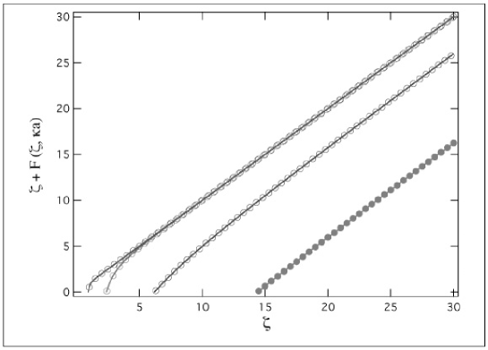
Figure 1: The $\zeta+F(\zeta)$ Eq. 57 for four different values of $\kappa a$, viz. $\kappa a=100,10,1$ and $0.1$ (from left to right). The dimensionless strength of the dipolar interaction $\left(\kappa\ell_{B}\right)\left(\frac{p_{0}}{e_{0}}\right)^{2}$ was taken as $1$. At large values of $\zeta$ the dependence is obviously linear.

Let us first of all introduce the following notation for the interaction potential

$$V_{R}(r) = \frac{p_{0}^{2}}{4\pi\epsilon\epsilon_{0}}\frac{e^{-\kappa r}}{r^{3}}(1+\kappa r)=v_{0}\kappa^{3}f_{R}(\kappa r)$$

$$V_{P}(r) = \frac{p_{0}^{2}}{4\pi\epsilon\epsilon_{0}}\frac{e^{-\kappa r}}{r^{5}}(3+3\kappa r+(\kappa r)^{2}))=v_{0}\kappa^{5}f_{P}(\kappa r),$$ (47)

where $f_{R,P}(u)$ are obviously defined as

$$f_{R}(u)=\frac{e^{-u}}{u^{3}}(1+u)$$

$$f_{P}(u)=\frac{e^{-u}}{u^{5}}(3+3u+u^{2}).$$ (48)

Introducing furthermore

$$\overline{\cal B}(z)=z-1+e^{-z}\quad{\rm with}\quad z=\frac{s}{\xi},$$ (49)

and setting

$$\overline{\xi}=1/(\sqrt{2}\kappa\xi),$$ (50)

we can derive the following form for $\delta K_{C}^{(1)}$

$$\delta K_{C}^{(1)}=-{\frac{v_{0}}{2}}(\kappa\xi)^{3}\int_{a/\xi}^{\infty}dzz^{2}\left(f_{R}\left(\sqrt{\overline{\cal B}(z)}/\overline{\xi}\right)-f_{P}\left(\sqrt{\overline{\cal B}(z)}/\overline{\xi}\right)\frac{\overline{\cal B}(z)}{\overline{\xi}^{2}}\right).$$ (51)

and for $\delta K_{C}^{(2)}$

$$\delta K_{C}^{(2)}=-\frac{v_{0}}{12}(\kappa\xi)^{5}\int_{a/\xi}^{\infty}dzz^{4}\left(f^{\prime}_{R}\left(\sqrt{\overline{\cal B}(z)}/\overline{\xi}\right)-f_{P}\left(\sqrt{\overline{\cal B}(z)}/\overline{\xi}\right)-f^{\prime}_{P}\left(\sqrt{\overline{\cal B}(z)}/\overline{\xi}\right)\frac{\overline{\cal B}(z)}{\overline{\xi}^{2}}\right)~{}e^{-z},$$ (52)

where the derivative in $f^{\prime}_{R}$ and $f^{\prime}_{P}$ stands for $f^{\prime}=\frac{\partial f(\sqrt{u})}{\partial u}$ and thus we have

$$f^{\prime}_{R}(u) = -\frac{e^{-u}}{2u^{5}}(3+3u+u^{2})$$

$$f^{\prime}_{P}(u) = -\frac{e^{-u}}{2u^{7}}(15+15u+6u^{2}+u^{3}).$$ (53)

We should again note here that the equations for the renormalized bending modulus Eqs. 51 and 52 are essentially non-linear, since $\delta K_{C}$ is also hidden in the variable $\overline{\xi}=dk_{B}T~{}/(4\sqrt{2}\kappa(K_{C}+\delta K_{C}))$.

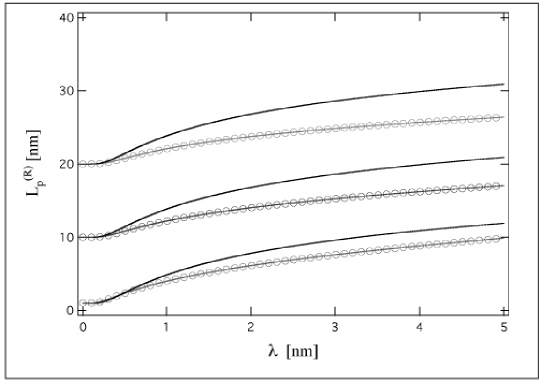
Figure 2: Renormalized persistence length Eq. 59 for three different values of $L_{p}^{(0)}=20,10$ and $1$nm (upper, middle, lower curves), circles. Also shown are the approximate solutions obtained from the expansion Eq. 63. The strength of the dipolar interaction $\ell_{B}\left(\frac{p_{0}}{e_{0}}\right)^{2}$ was taken as $1$ nm.

Let us finally introduce a new variable $\zeta$ defined as

$$\zeta=\overline{\xi}^{-1}=\sqrt{2}\kappa\xi=\frac{(4\sqrt{2}\kappa K_{C}^{(R)})}{3k_{B}T~{}}=\frac{4\sqrt{2}}{3}\frac{L_{p}^{(R)}}{\lambda_{D}},$$ (54)

where $\lambda_{D}=1/\kappa$ is the Debye screening length. $\zeta$ is nothing but the inverse reduced screeing length as introduced by Everaers et al. [3]. Furthermore if

$$\zeta^{(0)}=\frac{4\sqrt{2}\kappa K_{C}}{dk_{B}T~{}}\qquad{\rm and}\qquad\delta\zeta=\frac{4\sqrt{2}\kappa~{}\delta K_{C}}{dk_{B}T~{}}.$$ (55)

then the definition of the renormalized bending rigidity $K_{C}^{(R)}=K_{C}+\delta K_{C}$ can be cast into the form

$$\zeta=\zeta^{(0)}-\frac{\kappa v_{0}}{Dk_{B}T~{}}\zeta^{3}\left(F^{(1)}(\zeta)+\frac{\zeta^{2}}{12}F^{(2)}(\zeta)\right).$$ (56)

Because of Eq. 6 we can furthermore write in 3 dimensions

$$\zeta+F(\zeta)=\zeta+\textstyle{\frac{1}{3}}\left(\kappa\ell_{B}\right)\left(\frac{p_{0}}{e_{0}}\right)^{2}\zeta^{3}\left(F^{(1)}(\zeta)+{\textstyle{\frac{1}{12}}}\zeta^{2}F^{(2)}(\zeta)\right)=\zeta^{(0)}.$$ (57)

This equation gives the functional dependence of $\zeta$ on the parameters of the dipolar interaction, most notably $\lambda_{D}$. From the definition of $\zeta$ Eq. 54 the solution of the above equation immediately leads to the renormalized value of the persistence length. The functions $F^{(i)}(\zeta)$ have obviously been defined as

$$F^{(1)}(\zeta) = \int_{\sqrt{2}(\kappa a)/\zeta}^{\infty}dz~{}z^{2}\left(f_{R}\left(\zeta\sqrt{\overline{\cal B}(z)}\right)-f_{P}\left(\zeta\sqrt{\overline{\cal B}(z)}\right)\zeta^{2}\overline{\cal B}(z)\right)$$

$$F^{(2)}(\zeta) = \int_{\sqrt{2}(\kappa a)/\zeta}^{\infty}dz~{}z^{4}\left(f^{\prime}_{R}\left(\zeta\sqrt{\overline{\cal B}(z)}\right)-f_{P}\left(\zeta\sqrt{\overline{\cal B}(z)}\right)-f^{\prime}_{P}\left(\zeta\sqrt{\overline{\cal B}(z)}\right)\zeta^{2}\overline{\cal B}(z)\right)~{}e^{-z}.$$

(58)

Fig. 1 shows the dependence of $\zeta+F(\zeta)$ on $\zeta$ for four different values of $(\kappa a)$ that enters the definition of $F(\zeta)$ via the lower bound of the integrals Eq. 58. The solution of Eq. 57 is obtained from Fig. 1 by simply looking at the intersection between the curves on the figure with a line parallel to the $\zeta$ axis at $\zeta^{(0)}$.

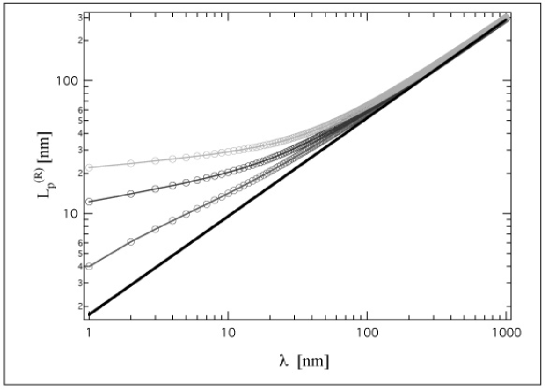
Figure 3: Fit (bold line)) of the renormalized persistence length to a power of $\lambda^{\alpha}$ for three different values of $L_{p}^{(0)}=1,10$ and $20$ nm (lower, middle and upper circles). The scaling exponent obtained from the fit is $\alpha=0.75$. The strength of the dipolar interaction $\ell_{B}\left(\frac{p_{0}}{e_{0}}\right)^{2}$ was taken as $1$ nm.

A more transparent form of these equations that will be solved numerically can be obtained if we go back to the original variables and can thus write for the renormalized persistence length

$$L_{p}^{(R)}=L_{p}^{(0)}-\frac{\ell_{B}}{4\sqrt{2}}\left(\frac{p_{o}}{e_{0}}\right)^{2}\left(\frac{4\sqrt{2}}{3}\frac{L_{p}^{(R)}}{\lambda_{D}}\right)^{3}\left(F^{(1)}\left(\frac{4\sqrt{2}}{3}\frac{L_{p}^{(R)}}{\lambda_{D}}\right)+{\textstyle{\frac{1}{12}}}\left(\frac{4\sqrt{2}}{3}\frac{L_{p}^{(R)}}{\lambda_{D}}\right)^{2}F^{(2)}\left(\frac{4\sqrt{2}}{3}\frac{L_{p}^{(R)}}{\lambda_{D}}\right)\right).$$ (59)

This equation is the main result of our paper. Its solution gives the renormalized value of the bending rigidity or equivalently the persistence length as a function of the dipolar interaction parameters. In general it can only be solved numerically but simplified analytic solutions can be obtained in limited regions of the paramater phase space.

It is instructive to compare these results with those derived for a polyelectrolyte chain with simple screened Debye - Hückel monopolar electrostatic interactions along the chain, where the fixed charges are at separation $A$ along the chain. If we formulate the results derived in in the same language as used above, we get

$$\zeta=\zeta^{(0)}+\frac{\sqrt{2}\kappa\ell_{B}}{12~{}2^{3}(A\kappa)^{2}}\zeta^{2}F(\zeta),$$ (60)

where in this case

$$F(\zeta)=\int_{0}^{\infty}dzz^{4}\left(1+\zeta\sqrt{\overline{\cal B}(z)}\right)\frac{e^{-\zeta}\sqrt{\overline{\cal B}(z)}}{{\overline{\cal B}(z)}^{{3/2}}}.$$ (61)

The analysis of these equations (though written in a somewhat different, yet completely equivalent form) has already been performed before and we direct the reader to that work [12].

6 Results

We noted already that the basic equations derived for the renormalization of the persistence length of a semiflexible dipolar chain have no simple analytic solution. Figures 2 and 3 thus present numerical solutions of Eq. 59 for some values of parameters $L_{p}^{(0)}$, $\lambda_{D}$, while we always consider the case $\frac{\ell_{B}}{2}\left(\frac{p_{o}}{e_{0}}\right)^{2}=1nm^{-1}$. This last parameter sets the overall scale of the renormalization and is not crucially significant so we do not study its variation in detail. Two universal behaviors seem to emerge. For small values of the screenenig length $\lambda_{D}$ the behavior is given in Fig. 2. For large values of the screening length an altogether different type of behavior is seen Fig. 3. Numerical solutions of Eq. 59 do not show any indications of a possible phase transition to an ordered phase at non-zero temperatures though due to the attractive component of the dipolar interactions one might expect them to. This is completely consistent with the behavior of the flexible chain [8].

Let us investigate if we can understand the two types of behavior depicted on Figs. 2 and 3 with simple analytical arguments. What we basically need to figure out is what would be the typical contributions to the integrals Eq. 58 that enter the equation for the renormalized bending rigidity Eq. 59. It is instructive to consider first the case of small screening lengths. Here the main contribution to the integrals Eq. 58 along the polyelectrolyte comes from short length scales. In this limit one derives that ${\cal B}(s)\simeq{s^{2}}$ and locally the chain thus behaves in the Kratky - Porod style [10]. This leads to the following approximate form of $F(\zeta)$

$$F(\zeta)=\zeta^{3}\left(F^{(1)}(\zeta)+\frac{\zeta^{2}}{12}F^{(2)}(\zeta)\right)=2\sqrt{2}\int_{\sqrt{2}(\kappa a)/\zeta}^{\sqrt{2}/\zeta}\frac{dz}{z}\left(-18-18\frac{\zeta z}{\sqrt{2}}-9\left(\frac{\zeta z}{\sqrt{2}}\right)^{2}+\left(\frac{\zeta z}{\sqrt{2}}\right)^{3}\right).$$ (62)

Eq. 59 in this very same limit then assumes the form

$$L_{p}^{(R)}=L_{p}^{(0)}-\frac{\ell_{B}}{2}\left(\frac{p_{o}}{e_{0}}\right)^{2}\left(\frac{(-25-7(\kappa a)+(\kappa a)^{2})e^{-(\kappa a)}}{12}-\frac{3}{2}E_{1}(\kappa a)\right),$$ (63)

where $E_{1}(u)$ is the standard exponential integral with a limiting form of $\lim_{u\longrightarrow 0}E_{1}(u)=-\gamma-\log{u}+{\cal O}(u)$. Except for very small values of the screening length where obviously $L_{p}^{(R)}\approx L_{p}^{(0)}$, a valid approximation of Eq. 63 capturing its dominant features would be

$$L_{p}^{(R)}\approx L_{p}^{(0)}+\frac{3\ell_{B}}{4}\left(\frac{p_{o}}{e_{0}}\right)^{2}\log{\frac{\lambda_{D}}{a}}.$$ (64)

This result could be seen as the dipolar chain equivalent of the Odijk - Skolnick - Fixman [2] result for the monopolar chain. In that case the behavior of the persistence length at small values of the screening length is $L_{p}^{(R)}\sim\lambda_{D}^{2}$. The difference between this result and Eq. 64 is purely due to the swifter decay of the dipolar interaction potential vs. separation, $r$, in monopolar case $r^{-1}$ and in dipolar case $r^{-3}$. This can be seen crudely as follows: since the interaction potential for the dipolar chain falls off twice as fast as the monopolar potential the OSF reasoning should give for the electrostatic persistence length $\lambda_{D}^{2}\times\lambda_{D}^{-2}=\lambda_{D}^{0}$. The zero in the exponent translates as usual into the $log$, which is exactly Eq. 64. The way the approximate result Eq. 63 fares when compared with the full numerical solution of Eq. 59 is shown on Fig. 2. Obviously the approximaton is not bad for small enough screening length but becomes progressively worse for larger bare persistence lengths and larger screening. The same reasoning applied to the general multipole of order $n$ would lead to the electrostatic persistence length with scaling $\lambda_{D}^{-(n-2)}$. One can thus hardly expect any electrostatic renormalisation effects above dipolar.

Next we consider the case of large(er) screening lengths. Here the main contribution to the integrals Eq. 58 along the polyelectrolyte comes from large(er) length scales. In this case the local properties of the chain are characterized by an essentially free flight behavior [10] of the chain, leading to ${\cal B}(s)\simeq 2\xi s$. Here we can derive

$$F(\zeta)=\zeta^{3}\left(F^{(1)}(\zeta)+\frac{\zeta^{2}}{12}F^{(2)}(\zeta)\right)=-\int_{\sqrt{2}(\kappa a)/\zeta}^{1/\zeta^{2}}dzz^{1/2}\left(2+2\zeta\sqrt{z}+\zeta^{2}z\right)=-\frac{41}{15}\zeta^{-3},$$ (65)

which leads to the following approximate form of Eq. 59

$$L_{p}^{(R)}\approx L_{p}^{(0)}+\frac{\ell_{B}}{4\sqrt{2}}\left(\frac{p_{o}}{e_{0}}\right)^{2}\frac{41}{15}\left(\frac{4\sqrt{2}}{3}\frac{L_{p}^{(R)}}{\lambda_{D}}\right)^{-3}=L_{p}^{(0)}+0.07~{}\ell_{B}\left(\frac{p_{o}}{e_{0}}\right)^{2}\left(\frac{\lambda_{D}}{L_{p}^{(R)}}\right)^{3}.$$ (66)

This equation can have two possible solutions depending on the magnitude of $L_{p}^{(0)}$. First of all if $L_{p}^{(R)}\gg L_{p}^{(0)}$, meaning that the value of the persistence length is determined mostly by the electrostatic interactions along the chain, we have

$$L_{p}^{(R)}=0.07^{1/4}\left(\ell_{B}\left(\frac{p_{o}}{e_{0}}\right)^{2}\right)^{1/4}\lambda_{D}^{3/4}.$$ (67)

This approximate result is nicely exhibited also on Fig. 3 where it is seen how the exact numerical solutions of Eq. 59 approach the above scaling limit for sufficiently large values of the screening length with the scaling exponent exactly equal to the above prediction. The form Eq. 67 is thus a limiting law for the electrostatic part of the persistence length valid universally for large screening lengths. One should be however aware, that in the above calculation by assumption the length of the chain is always the largest length in the system.

In the other case with a predominant contribution of the bare persistence length, i.e. $L_{p}^{(R)}\sim L_{p}^{(0)}$, thus in the limit where the strength of the dipolar interaction is very small, we end up with the following limiting form

$$L_{p}^{(R)}=L_{p}^{(0)}+0.07~{}\ell_{B}\left(\frac{p_{o}}{e_{0}}\right)^{2}\left(\frac{\lambda_{D}}{L_{p}^{(0)}}\right)^{3}.$$ (68)

The latter is only valid for small enough strength of the dipolar interaction and is difficult to discern in the numerical solution. Since all our numerical investigations on Figs. 2, 3 are based on the assumption of a fairly large strength of the dipolar interactions, this regime is not distinguishable on the graphs.

These last two results could again be compared with the expressions valid for the monopolar chain in the same regions of the parameter space and derived within the same theoretical framework [12]. In that case the behavior of the persistence length at large values of the screening length would be $L_{p}^{(R)}\sim\lambda_{D}^{\beta}$, where $\beta$ is either $7/6$ or $7$, depending on whether $L_{p}^{(R)}/L_{p}^{(0)}$ is either large or small. Again the difference between these results and Eqs. 67 and 68 is purely due to the swifter decay of the dipolar interaction potential vs. separation; monopolar case $r^{-1}$ and dipolar case $r^{-3}$. This difference introduces an additional factor of $\lambda_{D}^{-2}~{}\left(\frac{\lambda_{D}}{L_{p}^{(R)}}\right)^{-2}$ into the second term of Eq. 66, wherefrom the exponents $\beta=3/4$ or $3$ can be derived straightforwardly. It is thus clear that the behavior of the electrostatic part of the persistence length of a monopolar and dipolar chain are intimately related in both relevant limits of weak and strong screening. Applying again the same reasoning to the general multipole of order $n$ would lead to the electrostatic persistence length with scaling $\beta=(7-2n)$ or $\beta=(7-2n)/(6-n)$. Again electrostatic renormalisation effects above dipolar are very small.

The remaining question in this context would be how robust are the two regimes derived above that lead to the approximate forms Eqs. 64 and 67? In assessing the range of validity of these different approximations we can invoke a related situation already encountered in the case of a monopolar chain [12]. In that system extensive simulations [3, 4, 5] left no doubt that the OSF regime, corresponding in the context of the dipolar chain to Eq. 64, is very robust and extends over a broad region of the parameter phase space. The sub-OSF laws for the electrostatic renormalization of the persistence length giving $\beta$ in the vicinity of $1$ were effectively ruled out. Translating this into the context of the dipolar chain would make the range of validity fo Eq. 66 fairly narrow. But these are all conjectures since we are aware of no detailed simulations for semiflexible dipolar chains, setting aside the extensive work by Muthukumar on the flexible chain [8], that would match the superb work perfomed recently in the context of the monopolar chain [3, 4, 5].

7 Conclusions

We presented an analysis of the electrostatic contribution to the persistence length of a semiflexible screened-dipolar chain. The formal context of our analysis is provided by the $1/D$-expansion method that has been already successfully applied to different problems of polymer physics [12, 18, 19]. $1/D$-expansion is closely related to different variational schemes that have been amply applied to the problem of electrostatic rigidity of charged polymers [20, 21, 22, 23, 24]. What singles out our approach is the fact that we work consistently with a semiflexible Hamiltonian and enforce the inextensibility constraint on a global level. This leads to some discrepancies between variational formulations and $1/D$-expansion method. However the robustness of the OSF regime transpires quite clearly from the $1/D$-expansion in the context of a monopolar polyelectrolyte, giving us some confidence that an analogous result for a dipolar chain would have the same range of validity.

The main step in our formulism was to find an appropriate way to treat the orientational dependence of the intersegment interaction potential. This has been accomplished by introducing additional auxiliary fields that in their turn lead to new saddle-point equations. Though the derivation of the renormalized elasticity is as a consequence more complicated, it leads to manageable and transparent results. The main conclusion based on these results would be that the dependence of the electrostatic persistence length on the screening length for a dipolar chain is much less pronounced then for a monopolar chain. This is clearly seen in the case of large as well as small screening. Also it appears that a semiflexible chain does not give rise to any localized structures as those described by Muthukumar [8] in the context of a flexible chain. This is indeed not surprising since the chain elasticity is obviously strong enough to prevent extensive looping of the chain that would lead to local aggregation of the chain based on the attractive component of the dipolar interaction. This attractive component is also not strong enough to lead to any type of phase transition to an ordered state at non-zero temperatures. This conclusion is just as valid for a semiflexible as it is for a flexible chain.

Eventually the conclusions arrived at in this work would have to be tested against extensive simulations just as they were in the case of a monopolar charged chain. As for the experimental situation where repeated claims of a sub-OSF regime have been voiced [25, 26], one wonders if they could in fact be a consequence of a specific association of the mobile counterions with fixed charges on the polyelectrolyte backbone producing a system not far from the model dipolar chain analyzed in this work. In order to test this hypothesis one would have to estimate independently the effective dipole moments of the chain segments. The results presented in this work could then serve as a guideline to differentiate between monopolar and dipolar OSF-like behavior.

Acknowledgment I would like to thank Per Lyngs Hansen for numerous discussions regarding polyelectrolytes and their theoretical description.

References

- [1] Yamakawa H, Helical Wormlike Chains in Polymer Solutions (Springer Verlag: New York) 1997.
- [2] Odijk, T. J. Polym. Sci. 15 (1977) 477-483.. Skolnick J, Fixman M Macromolecules 10 (1977) 944-948.
- [3] Everaers R, Milchev A, Yamakov V Eur Phys J E 8 (2002) 3-14.
- [4] Ullner M J Phys Chem B 107 (2003) 8097-8110.
- [5] Nguyen TT and Shklovskii BI Phys Rev E 66 (2002) 021801.
- [6] Popov A, Hoagland DA (2004) personal communication.
- [7] Eisenberg A, Kim J-S, Introduction to Ionomers (Wiley-Interscience; 1 edition) 1998.
- [8] Muthukumar M J Chem Phys 104 (1996) 691-700.
- [9] Lodge TP, Muthukumar M J Phys Chem 100 (1996) 13275-13292.
- [10] Rubinshtein M and Colby RH, Polymer Physics (Oxford University Press, Oxford) 2003.
- [11] Polyakov AM, Gauge Fields and Strings (Contemporary Concepts in Physics, Vol 3) ( Taylor and Francis) 1987.
- [12] Hansen PL and Podgornik R J Chem Phys 114 (2001) 8637-8648.
- [13] Barrat, J-L, Joanny, J-F Adv. Chem. Phys 94 (1996) 1-66.
- [14] Schwinger JS, Deraad LL, Milton KA, Tsai WY Classical Electrodynamics (Perseus Books Group) 1998.
- [15] Pitard E, Garel T, Orland H Journal de Physique I 7 (1997) 1201-1210.
- [16] Kamien RD Reviews of Modern Physics 74 (2002) 953-971.
- [17] Gupta AM, Edwards SF J Chem Phys 98 (1993) 1588-1596.
- [18] Podgornik R, Hansen PL, Parsegian VA J Chem Phys 113 (2000) 9343-9350.
- [19] Hansen PL, Svensek D, Parsegian VA, , Podgornik R Phys Rev E 60 (1999) 1956-1966.
- [20] Podgornik R J Chem Phys 99 (1993) 7221-7231.
- [21] Bratko D, Dawson KA J Chem Phys 99 (1993) 5352-5361.
- [22] Li H, Witten TA Macomol 28 5921-5927.
- [23] Netz RR, Orland H Eur Phys J B 8 (1999) 81-98.
- [24] Ha BY, Thirumalai D Macromol 36 (2003) 9658-9666.
- [25] Reed WF, Ghosh S, Medjahdi G, Francois J Macromol 24 (1991) 6189-6198.
- [26] Beer M, Schmidt M, Muthukumar M Macromol 30 (1997) 8375-8385.