Accelerated dynamics with the dynamical activation-relaxation technique

Abstract

The dynamics of many atomic systems is controlled by activated events taking place on a time scale which is long compared to that associated with thermal vibrations. This often places problems of interest outside the range of standard simulation methods such as molecular dynamics. We present here an algorithm, the dynamical activation-relaxation technique (DART), which slows down thermal vibrations, while leaving untouched the activated processes which constitute the long-time dynamics. As an example, we show that it is possible to accelerate considerably the dynamics of self-defects in a 1000-atom cell of c-Si over a wide range of temperatures.

Developing algorithms that stretch the time scale accessible to computer simulations has been a major challenge in computational physics, chemistry and biology. Standard techniques such as molecular dynamics are strongly constrained by the presence of high-frequency modes in dense materials and must therefore use an integration time step on the order of a femtosecond, limiting the simulation length to microseconds at best. Over the years, a number of accelerated algorithms have been proposed for discrete systems where it is possible to enumerate, in advance, all the possible barriers. The original ideas for these algorithms are due to Bortz, Kalos and Lebowitz Bortz et al. (1975). They were first applied to MBE growth in 1986 by Voter Voter (1986). This method and many variants are now common simulation techniques in surface science.

Algorithmic progress has been much slower for systems in which either the number of pathways, or their activation energies, change all the time. Many methods have been proposed for sampling events efficiently  Barkema and Mousseau (1996); Mousseau and Barkema (1998); Malek and Mousseau (2000); Doye and Wales (1997); Henkelman and Jónsson (1999); Iannuzzi et al. (2003); Bolhuis et al. (2000); Mousseau and Barkema (2004) but only a few of these can provide a time scale: hyper-molecular dynamics and related approches Voter (1997); Miron and Fichthorn (2003) as well as temperature-assisted dynamics, introduced by Sorensen and Voter Sorensen and Voter (2000), are limited to systems with a relatively narrow distribution of barriers and cannot be used easily at high temperatures or on generic problems. Other methods, such as a kinetic Monte Carlo scheme with on-the-fly calculation of the barriers Henkelman and Jónsson (2001) generate impressive acceleration. However, their application is limited to relatively simple systems, and entropic effects are not fully included, hence detailed balance cannot be ensured.

In this paper, we present an algorithm, the dynamical activation-relaxation technique (DART), with a self-correcting accelerating factor that can reach a few orders of magnitude at physically relevant temperatures while overcoming some of the limitations of these accelerated methods. It is based on the thermodynamically-weighted activation-relaxation technique (THWART) which we introduced recently Mousseau and Barkema (2004), and combines molecular dynamics with Monte Carlo methods to reach a dynamically correct acceleration of the slow processes in complex materials. In order to assess the efficiency of DART, we apply the method to the diffusion of vacancies and interstitials in c-Si.

The energy landscape of systems with dynamics controlled by rare events can be divided into two types of subregions, as shown in Fig. 1: the basins, closed regions of the energy landscape, in which the system is confined for extended periods and which can contain many local minima, and the “activated part of phase space”, sampled only when a rare fluctuation pushes the system from one basin to another. Following THWART, we delineate the basins based on the value of the lowest local curvature of the energy landscape (i.e., the lowest eigenvalue of the hessian matrix); any configuration with a lowest curvature below the threshold is considered to be in the saddle region. The exact threshold value depends on the system studied as well as on the simulation temperature.

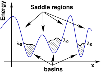
Figure 1: The energy landscape of systems with a long-time dynamics determined by activated events.

The simulation starts with standard molecular dynamics in a microcanonical ensemble. After equilibration, the MD run is pursued but with regular evaluation of the lowest local curvature $\lambda_{0}$. As long as $\lambda_{0}$ remains above a threshold value $\lambda_{t}$, the system is considered to reside in the original basin. As soon as this threshold is reached, however, the activation phase of THWART is launched: the MD simulation is stopped, the current velocities stored and the system is moved from one basin to another. The step is designed to bring the configuration from the edge of a basin to that of a neighboring one, in a fully reversible manner and at constant potential energy in order to respect detailed balance; it is identical to that used in THWART. Each activation move consists of a sequence of small steps with size $\Delta x$, defined as follows:

$$\vec{x}_{i+1}=\vec{x}_{i}+\frac{\Delta x}{2}\left(\vec{h}_{i+1}+\vec{h}_{i}\right)+c\left(\vec{F}^{\perp}_{i+1}+\vec{F}^{\perp}_{i}\right),$$ (1)

where $\vec{h}$ is the direction of lowest curvature and $\vec{F}^{\perp}$ is the force perpendicular to this vector; $c$ is a scalar tuned at each step to keep the total configurational energy constant. The orientation of $\vec{h}_{0}$ is chosen away from the basin, while successive orientations are chosen such that $\vec{h}_{i+1}\cdot\vec{h}_{i}>0$. This step is repeated until the lowest curvature of the energy landscape reaches again the threshold value $\lambda_{t}$. Note that each individual step, and hence the whole trajectory, is fully reversible. Since each activation move connects two points in phase space with the same potential energy and since the Jacobian of transformation is equal to one Mousseau and Barkema (2004), detailed balance is fully respected. Within THWART, activated moves are always accepted; the MD is therefore continued from the end of the activation path using the stored velocities, ready for a new activation.

THWART ensures a proper thermodynamical sampling of the phase space; the THWART trajectory, however, does not follow the real dynamics. In particular, it crosses highly activated pathways as easily as those with a low activation barrier. In order to recover the actual dynamics, it is necessary to first determine the height of the barriers crossed. By construction, activation pathways have constant energy and the deformation energy stored in the degrees of freedom not directly involved in the activation process is used as a bath to enforce this constraint. It is nevertheless straightforward to to determine the energy associated with the diffusion path: the total force is split into a component parallel to the direction of lowest curvature ($\vec{F}^{\parallel}$) and a component perpendicular to this direction ($\vec{F}^{\perp}$), at each step along the activation trajectory; using the first component, the change in total energy due to the parallel displacement is written

$$\Delta E^{\parallel}\equiv-\int\vec{F}^{\parallel}\cdot d\vec{R}.$$ (2)

The activation energy barrier (from the edge of the basin) is then defined as the change in energy from the edge of the basin to the maximum energy change projected along this path.

The probability that the kinetic energy at the beginning of the activation trajectory suffices to bring the configuration over the barrier through this highest point is given by $\exp(-\beta\max(\Delta E^{\parallel}))$, with inverse temperature $\beta=1/(k_{b}T)$. Assuming around each first-order saddle point a quadratic behavior of the energy in the transition plane, the energy at the nearest saddle point will on average be $\frac{1}{2}k_{b}T$ lower. We therefore take for the activation barrier, faced from the basin boundary:

$$\Delta E_{\rm act}=\max(\Delta E^{\parallel})-\frac{1}{2}k_{b}T.$$ (3)

To retrieve the dynamics in a statistically correct manner, we should accept the activation move with probability $\exp(-\beta\Delta E_{\rm act})$, and otherwise continue in the original basin. Typically in a system with activated dynamics, these acceptance probabilities are rather small, and the system will bounce back and forth in the basin many times before eventually escaping from it; hence the slow dynamics. However, the speed of the simulation can be enhanced by a (constant) nominal boost factor $X_{b}$ reducing the number of such bounces. The acceptance probability for an activation pathway then becomes

$$P_{\rm cross}=\min\left[1,X_{b}\exp\left(-\beta\Delta E_{\rm act}\right)\right].$$ (4)

If, on top of boosting the acceptance probabilities by a factor of $X_{b}$, the time scale is stretched by the same factor, the long-time dynamics is untouched, provided it is indeed determined by activated processes with barriers exceeding $\ln(X_{b})k_{b}T$, while the suppression of the in-basin dynamics (by a factor $X_{b}$) as well as the suppression of less activated processes (by a smaller factor) does not affect the long-time dynamics. Once barriers below $\ln(X_{b})k_{b}T$ are encountered, inevitably some distortion of the dynamics occurs. To alleviate the distortion somewhat, if we encounter such a low barrier, we stretch the time scale since the previous event by an on-the-fly corrected boost factor

$$X_{\rm eff}=P_{\rm cross}\cdot\exp(\beta\Delta E_{\rm act}),$$ (5)

rather than the nominal boost factor $X_{b}$; this recovers correct dynamics for systems in which the activation energy is constant, even if the chosen nominal boost factor is too large.

A DART simulation proceeds in the following sequence: (1) at time $t=0$, a microcanonical molecular dynamics simulation is launched and the value of the lowest local curvature $\lambda_{0}$ is monitored at regular intervals (typically, every 50 steps); (2) when $\lambda_{0}$ reaches the threshold value $\lambda_{t}$, the molecular dynamics is stopped and the velocities are saved; (3) following Eq. (1) iteratively, the configuration is brought into a new basin and the activation energy $\Delta E_{\rm act}$ is computed along the activated pathway; (4) the event is accepted with probability $P_{\rm cross}$; (5) if the event is accepted, the time is incremented by $\Delta t=t_{\rm MD}\cdot X_{\rm eff}$, in which $t_{\rm MD}$ is the time spent doing molecular dynamics since the previous accepted event, and the molecular dynamics simulation is continued starting at the new edge with the same velocities. If it is rejected, the molecular dynamics simulation is simply continued from the initial edge.

To demonstrate the efficiency of DART, we consider the diffusion of vacancies and interstitials in c-Si, described by the Stillinger-Weber potential. Both types of defects have been well characterized previously Maroudas and Brown (1993); Nastar et al. (1996). Vacancy diffusion is associated with a single activation barrier of 0.43 eV Maroudas and Brown (1993). An interstitial can take four different stable topologies: tetrahedral, hexagonal, bond-centered and split or dumbbell. It diffuses through many mechanisms with activation barriers between 0.65 and 1.62 eV Nastar et al. (1996). Therefore, these two defects provide us with various levels of complexity to test DART.

Figure  2 shows an Arrhenius plot of the diffusion rates obtained by MD and by DART with various boost factors. We characterize the diffusion rates by the hopping rates of the defects, which gives better statistics than the mean squared displacements per unit of time. As can be seen, an excellent agreement between the two methods is achieved for both the vacancy, characterized by a single energy barrier, and for the interstitial, which shows a more complex behavior.

As mentioned above, DART adjusts automatically for barriers lower than $\ln(X_{b})k_{b}T$. Table  1 gives the nominal and effective boost factors for the various DART simulations plotted in Fig.  2. As expected, the gain in efficiency increases rapidly with decreasing temperature. From a factor of 1 at about 1100K (not shown), the effective boost for interstitial diffusion reaches 10 at 900 K, 74 at 750 K and almost 150 at 600 K, an experimentally relevant temperature. The extra computational effort in DART is largely due to the computation of the lowest curvature, both at regular intervals and during the THWART events. Averaged over the whole simulation, with an evaluation at every 50 MD steps, a DART time step costs slightly less than two MD time steps.

Figure 2: Diffusion rate as a function of inverse temperature for vacancy (top) and the interstitial (bottom) diffusion in Si. The open circles represent MD results and the squares DART results. Error bars are obtained from the square root of the total number of events. The nominal and averaged effective boost factors for these simulations are given in Table  1.

Table 1: Details of the various DART simulations

Defect	Temperature	$\lambda_{0}$	Boost
	(K)	(eV/ Å2)	Nominal	Effective
Vacancy	900	-5	6	3.6
	900	-5	30	6.7
	600	-5	6	5.4
	600	-5	30	19
	450	-5	600	271
Interstitial	900	-7	60	10
	750	-7	600	74
	600	-7	1200	148

In conclusion, we have presented here an accelerated molecular dynamical method – the dynamical activation-relaxation method (DART). This algorithm provides a tunable acceleration parameter that can be adjusted to suit the specific problems studied. In addition to providing a significant acceleration over MD, DART has numerous advantages: (1) the algorithm is not very sensitive to the various parameters - it can automatically correct for boost factors an order of magnitude or more too large; (2) it computes relaxation trajectories and activation barriers on the fly, leading to a very low overhead (on average, a DART time step is less than twice the cost of an MD time step); (3) DART is not slowed down by the local rearrangements which take place in the basin (i.e, below threshold) — contrary to other accelerated methods, it is therefore possible to use DART to accelerate the dynamics of more complex systems such as glasses and proteins; (4) since the events are easily labeled, it is possible to use various tricks to avoid repeating the same event over and over again – this can lead to a large increase in efficiency; finally, (5) the limits of DART are well behaved: a zero-boost reduces DART to standard MD, while an infinite boost factor recovers THWART and still ensures proper thermodynamical sampling.

Tests on a vacancy and an interstitial in c-Si have shown that this method remains accurate dynamically with an increased computational efficiency of two or more orders of magnitude, at temperatures as high as 450 K for the vacancies or 600 K for interstitial diffusion. As mentioned above, however, this method can also be applied to much more complex situations where current accelerated algorithms fail.

Acknowledgements. NM is supported in part by FQRNT and NSERC. We are grateful to the RQCHP for generous allocation of computer resources. NM is a Cottrell Scholar of the Research Corporation.

References

- Bortz et al. (1975) A. Bortz, M. H. Kalos, and J. Lebowitz, J. Comp. Phys. 17, 10 (1975).
- Voter (1986) A. F. Voter, Phys. Rev. B 34, 6819 (1986).
- Barkema and Mousseau (1996) G. T. Barkema and N. Mousseau, Phys. Rev. Lett. 77, 4358 (1996).
- Mousseau and Barkema (1998) N. Mousseau and G. T. Barkema, Phys. Rev. E 57, 2419 (1998).
- Malek and Mousseau (2000) R. Malek and N. Mousseau, Phys. Rev. E 62, 7723 (2000).
- Doye and Wales (1997) J. Doye and D. Wales, Z. Phys. D Atom. Mol. Cl. 40, 194 (1997).
- Henkelman and Jónsson (1999) G. Henkelman and H. Jónsson, J. Chem. Phys 111, 7010 (1999).
- Iannuzzi et al. (2003) M. Iannuzzi, A. Laio, and M. Parrinello, Phys. Rev. Lett. 90, 238302 (2003).
- Bolhuis et al. (2000) P. G. Bolhuis, C. Dellago, P. L. Geissler, and D. Chandler, J. Phys. Cond. Matt. 12, A147 (2000).
- Mousseau and Barkema (2004) N. Mousseau and G. T. Barkema, submitted to Phys. Rev. Lett. (2004).
- Voter (1997) A. F. Voter, Phys. Rev. Lett. 78, 3908 (1997).
- Miron and Fichthorn (2003) R. A. Miron and K. A. Fichthorn, J. Chem. Phys 119, 6210 (2003).
- Sorensen and Voter (2000) M. Sorensen and A. F. Voter, J. Chem. Phys. 112, 9599 (2000).
- Henkelman and Jónsson (2001) G. Henkelman and H. Jónsson, J. Chem. Phys 115, 9657 (2001).
- Maroudas and Brown (1993) D. Maroudas and R. A. Brown, Phys. Rev. B 47, 15562 (1993).
- Nastar et al. (1996) M. Nastar, V. V. Bulatov, and S. Yip, Phys. Rev. B 53, 13521 (1996).