Spectroscopy of Superfluid Pairing in Atomic Fermi Gases

Abstract

We study the dynamic structure factor for density and spin within the crossover from BCS superfluidity of atomic fermions to the Bose-Einstein condensation of molecules. Both structure factors are experimentally accessible via Bragg spectroscopy, and allow for the identification of the pairing mechanism: the spin structure factor allows for the determination of the two particle gap, while the collective sound mode in the density structure reveals the superfluid state.

Atomic fermions have attracted a lot of interest as current cooling techniques allow for the creation of molecular condensates Jochim et al. (2003); Greiner et al. (2003); Zwierlein et al. (2003); Salomon (2003). These superfluids behave very much like standard Bose-Einstein condensates (BEC): the condensate may be inferred from the momentum distribution measured in a time of flight experiment. The tunability of the interaction through a Feshbach resonance then offers the possibility to explore the crossover from BEC of tightly bound molecules to the BCS superfluid state, where Cooper pairs only exist due to many body effects Nozières and Schmitt-Rink (1985); Randeria and Shieh (1990); Haussmann (1993); Pistolesi and Strinati (1994); Holland et al. (2001); Ohashi and Griffin (2002). Recent experiments have entered this regime Regal et al. (2004); bla (2004); Bartenstein et al. (2004), however, clear signatures for extended Cooper pairs in a BCS like ground state are missing so far. In this letter, we present a generalization of available spectroscopic tools to measure the dynamic structure factor for density and spin, which reveal important information on the pairing mechanism within the BEC-BCS crossover.

In conventional superconductors, the main characteristic properties are dissipation free transport and the Meissner-Ochsenfeld effect, which reveal themselves in the current response; density fluctuations are suppressed due to long-range Coulomb interactions Schrieffer (1964) (see Ref. Pistolesi and Strinati (1994) for the current response in the BEC-BCS crossover). In contrast, for uncharged atomic gases transport measurements are not readily accessible due to the trapping potential. Then, the dynamic structure factors for density and spin are suitable quantities for the characterization of the superfluid ground state within the BEC-BCS crossover. Both quantities are accessible in traps: recent experiments measured the dynamic structure factor in interacting Bose gases via Bragg spectroscopy Stamper-Kurn et al. (1999); Steinhauer et al. (2002); Stöferle et al. (2003), while the dynamic spin susceptibility may be inferred by measuring the spin flip rate in stimulated Raman transitions Törmä and Zoller (2000); Grimm and Chin (private discussion). In this paper, we analyze the dynamic structure factor $S_{\rm\scriptscriptstyle C}$ and the dynamic spin structure factor $S_{\rm\scriptscriptstyle S}$ within the BEC-BCS crossover. We find, that the dynamic spin structure factor is dominated by processes which break paired fermions into two single particles and therefore reveals the many-body excitation gap. Furthermore, it provides the density of states, which signals the BCS pairing mechanism via the the appearance of a van Hove singularity. The observation of this singularity was a fundamental indication for the validity of BCS theory in conventional superconductors Schrieffer (1964). In turn, the superfluid transition is characterized by the appearance of a collective sound mode in the dynamic structure factor; this collective mode has recently been studied Minguzzi et al. (2001); Ohashi and Griffin (2002); hofstetter (2002).

An interacting atomic gas of fermions with density $n_{\rm\scriptscriptstyle F}=k_{\rm\scriptscriptstyle F}^{3}/3\pi^{2}$ and two different spin states is characterized by the scattering length $a_{\rm\scriptscriptstyle F}$ allowing to tune the BEC-BCS crossover via the dimensionless parameter $1/(k_{\rm\scriptscriptstyle F}a_{\rm\scriptscriptstyle F})$. As shown by Nozières and Schmitt-Rink Nozières and Schmitt-Rink (1985), the BCS wave function becomes exact in the BCS limit ($1/(k_{\rm\scriptscriptstyle F}a_{\rm\scriptscriptstyle F})\ll-1$) and the BEC limit ($1/(k_{\rm\scriptscriptstyle F}a_{\rm\scriptscriptstyle F})\gg 1$). In the following, we use this BCS wave function to determine the dynamic structure factor $S_{\rm\scriptscriptstyle C}$ from the density response function $\chi_{\rm\scriptscriptstyle C}$, and the dynamic spin structure factor $S_{\rm\scriptscriptstyle S}$ from the spin susceptibility $\chi_{\rm\scriptscriptstyle S}$. This wave function accounts for the pairing between two fermions, while the residual interaction between unbound fermions providing particle-hole scattering is neglected. The interaction between molecules (Cooper pairs) is accounted for within Born approximation Randeria and Shieh (1990) (it is not necessary to introduce a molecular field as done in Ref. Ohashi and Griffin (2002)). Within the BCS variational wave function, the fermionic normal Green’s function $\mathcal{G}$ and the anomalous Green’s function $\mathcal{F}^{+}=-\mathcal{F}$ take the standard form Schrieffer (1964)

$$\mathcal{G}(\Omega_{s},{\bf k})\!=\!\frac{i\Omega_{s}\!+\!\epsilon_{\bf k}}{(i\Omega_{s})^{2}\!-\!E_{\bf k}^{2}},\hskip 15.0pt\mathcal{F}^{+}(\Omega_{s},{\bf k})\!=\!\frac{-i\Delta}{(i\Omega_{s})^{2}\!-\!E_{\bf k}^{2}}.$$

Here, $E_{\bf k}=\sqrt{\epsilon_{\bf k}^{2}+\Delta^{2}}$ denotes the single-particle excitation energy with $\epsilon_{\bf k}=\hbar^{2}{\bf k}^{2}/2m-\mu$ the free fermionic dispersion relation, while $\Omega_{s}=\pi T(2s+1)$ denotes fermionic Matsubara frequencies. The presence of a condensate and superfluid response in the ground state is encoded in a finite BCS gap $\Delta$. The gap $\Delta$ is determined by the scattering length $a_{\rm\scriptscriptstyle F}$ via the gap equation, and the chemical potential is fixed by the particle density $n_{\rm\scriptscriptstyle F}$ Randeria and Shieh (1990),

$$-1 = \frac{4\pi\hbar^{2}a_{\rm\scriptscriptstyle F}}{m}\int\frac{d{\bf q}}{(2\pi)^{3}}\left[\frac{\tanh\left(\beta E_{\bf q}\right/2)}{2E_{\bf q}}-\frac{m}{\hbar^{2}{\bf q}^{2}}\right],$$ (1)

$$n_{\rm\scriptscriptstyle F} = 2\int\frac{d{\bf q}}{(2\pi)^{3}}\left[\frac{1}{1+e^{\beta E_{\bf q}}}\frac{\epsilon_{\bf q}}{E_{\bf q}}+\frac{E_{\bf q}-\epsilon_{\bf q}}{2E_{\bf q}}\right].$$ (2)

In the BCS limit at low temperatures ($T=0$), these relations give the chemical potential $\mu=\epsilon_{\rm\scriptscriptstyle F}$ and the gap $\Delta=\epsilon_{\rm\scriptscriptstyle F}(8/e^{2})\exp\big{(}\pi/2k_{\rm\scriptscriptstyle F}a_{\rm\scriptscriptstyle F}\big{)}$ with $\epsilon_{\rm\scriptscriptstyle F}$ the Fermi energy. In turn, in the BEC limit the appearance of a two particle bound state with binding energy $\epsilon_{0}=\hbar^{2}/(ma_{\rm\scriptscriptstyle F}^{2})$ and internal wave function $\phi_{\bf k}=(2n_{\rm\scriptscriptstyle F})^{-1/2}\Delta/E_{\bf k}$ modifies the chemical potential $\mu=-\epsilon_{0}/2$ and the gap $\Delta=\epsilon_{0}\sqrt{4\pi n_{\rm\scriptscriptstyle F}a_{\rm\scriptscriptstyle F}^{3}}$. Within the crossover regime, we solve Eq. (1) and (2) numerically to determine $\Delta(k_{\rm\scriptscriptstyle F}a_{\rm\scriptscriptstyle F})$ and $\mu(k_{\rm\scriptscriptstyle F}a_{\rm\scriptscriptstyle F})$. Note, that in general the BCS gap $\Delta$ differs from the two particle excitation gap $\Delta_{\rm\scriptscriptstyle S}=\min_{\rm\scriptscriptstyle{\bf k}}2E_{\bf k}$.

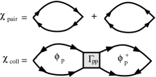
Figure 1: Diagrams contributing to the density response function and the spin susceptibility; $\chi_{\rm\scriptscriptstyle pair}$ accounts for particle-hole excitations, while the diagrams in $\chi_{\rm\scriptscriptstyle coll}$ describe collective sound excitations.

In the following, we calculate the dynamic structure factor $S_{\rm\scriptscriptstyle C}=-{\rm Im}\chi_{\rm\scriptscriptstyle C}/\pi$ and the dynamic spin structure factor $S_{\rm\scriptscriptstyle S}=-{\rm Im}\chi_{\rm\scriptscriptstyle S}/\pi$ via their relations to the density response function and the spin susceptibility, respectively. The density response $\delta\rho_{\rm\scriptscriptstyle C}(\omega,{\bf k})$ to a small external drive $\delta V_{\rm\scriptscriptstyle C}(\omega,{\bf k})$ follows from $\delta\rho_{\rm\scriptscriptstyle C}(\omega,{\bf k})=\chi_{\rm\scriptscriptstyle C}(\omega,{\bf q})\delta V_{\rm\scriptscriptstyle C}(\omega,{\bf k})$ with the linear response function (in real space)

$$\chi_{\rm\scriptscriptstyle C}(t,{\bf x})=-i\Theta(t)\langle\left[\rho_{\rm\scriptscriptstyle C}(t,{\bf x}),\rho_{\rm\scriptscriptstyle C}(0,0)\right]\rangle.$$ (3)

Here, $\langle\ldots\rangle$ denotes the quantum statistical average at fixed temperature $T$ and chemical potential $\mu$, while the density operator is defined by $\rho_{\rm\scriptscriptstyle C}=\psi^{+}_{\uparrow}\psi_{\uparrow}+\psi^{+}_{\downarrow}\psi_{\downarrow}$. The analogous definition applies for the spin susceptibility with the density $\rho{\rm\scriptscriptstyle C}$ replaced by the spin density $\rho_{\rm\scriptscriptstyle S}=\psi^{+}_{\uparrow}\psi_{\uparrow}-\psi^{+}_{\downarrow}\psi_{\downarrow}$. The diagrams contributing to the response functions $\chi_{\rm\scriptscriptstyle C}$ and $\chi_{\rm\scriptscriptstyle S}$ are shown in Fig. 1. Note, that each diagram has to be weighted by a nontrivial factor $\pm 1$. These factors differ for the response function $\chi_{\rm\scriptscriptstyle C}$ and the spin susceptibility $\chi_{\rm\scriptscriptstyle S}$, and provide different cancellations between diagrams. We distinguish between two types of diagrams: The first type of diagrams $\chi_{\rm\scriptscriptstyle pair}$ involve only normal and anomalous Green’s function and describe two particle excitations, while the second type of diagrams $\chi_{\rm\scriptscriptstyle coll}$ involve the vertex operator $\Gamma_{\alpha\beta}$ and account for collective excitations. The BCS wave function neglects particle-hole scattering and $\Gamma$ accounts only for particle-particle (hole-hole) scattering. Then, $\alpha,\beta\in\{p,\overline{p}\}$ describe the incoming and outgoing type of particles; $p$ accounts for particles and $\overline{p}$ for holes. The vertex operator $\Gamma$ has to be calculated with the help of the BCS wave function, see below. Note, that Fig. 1 shows only the diagram involving $\Gamma_{pp}$, while the other diagrams exhibit a similar structure. In the following, we are mainly interested in the zero temperature limit $T=0$ and in the low momentum regime $k\ll 1/\xi=\Delta/\hbar c_{s}$ (the energy of the collective modes is below the two particle gap $\omega<\Delta_{\rm\scriptscriptstyle S}$). Here, $c_{s}$ denotes the macroscopic sound velocity and $\xi$ the size of the pairs with $\xi\sim\hbar v_{\rm\scriptscriptstyle F}/\Delta$ in the BCS limit and $\xi\sim a_{\rm\scriptscriptstyle F}$ in the BEC limit. For typical experimental setups, the scale $\xi$ is small compared to the trap size $R$, and we can safely assume the condition $1/R<k<1/\xi$. Then, the trapping potential plays a minor role as has been shown in the measurement of the dynamic structure factor and the tunnelling probability, see Ref. Stamper-Kurn et al. (1999); Steinhauer et al. (2002); Grimm and Chin (private discussion). Therefore, we ignore the influence of a trapping potential in the following analysis.

First, we focus on the spin susceptibility $\chi_{\rm\scriptscriptstyle S}$. At zero momentum, the spin susceptibility $\chi_{\rm\scriptscriptstyle S}(\omega,0)$ is equivalent to the response driven by the spin flip Hamiltonian $H=\lambda(t)\int d{\bf x}\big{[}\psi^{+}_{\uparrow}\psi_{\downarrow}+\psi^{+}_{\downarrow}\psi_{\uparrow}\big{]}$. A perturbation of this form is realized experimentally by driving a stimulated Raman transition between the two hyperfine states of the two component Fermi gas Grimm and Chin (private discussion). Within the diagrammatic expansion of $\chi_{\rm\scriptscriptstyle S}$, the diagrams in $\chi_{\rm\scriptscriptstyle coll}$ cancel each other and only pair excitations $\chi_{\rm\scriptscriptstyle pair}$ survive; their contribution takes the form

$$\chi_{\rm\scriptscriptstyle S}(\Omega_{s},{\bf k})\!\!\! = \!\!-2T\sum_{t\in{\bf Z}}\int\frac{d{\bf q}}{(2\pi)^{3}}\Big{[}\mathcal{G}(\Omega_{t},{\bf q})\mathcal{G}(\Omega_{s+t},{\bf q+k})$$ (4)

$$\hskip 40.0pt+\mathcal{F}^{+}(\Omega_{t},{\bf q})\mathcal{F}(\Omega_{s+t},{\bf q+k})\Big{]}$$

(Note, that for the density response function $\chi_{\rm\scriptscriptstyle C}$ the $+$ sign between the two terms is replaced by a $-$ sign Schrieffer (1964).) The integration in (4) involves standard methods, and we present here only the final result for the spin structure factor in the low momentum limit $k\ll 1/\xi$, see Fig. 2,

$$S_{\rm\scriptscriptstyle S}(\omega)\!=\!\frac{3}{4}\frac{(n_{\rm\scriptscriptstyle F}/\epsilon_{\rm\scriptscriptstyle F})\Delta^{2}}{\omega\sqrt{\left(\hbar\omega/2\right)^{2}\!-\!\Delta^{2}}}\left[\frac{\sqrt{\left(\hbar\omega/2\right)^{2}\!-\!\Delta^{2}}\!+\!\mu}{\epsilon_{\rm\scriptscriptstyle F}}\right]^{1/2}.$$ (5)

The spin structure factor exhibits a gap $\Delta_{\rm\scriptscriptstyle S}=2\min_{\rm\scriptscriptstyle{\bf k}}E_{\bf k}$, i.e., for positive $\mu$ the spin gap $\Delta_{\rm\scriptscriptstyle S}=2\Delta$ is determined by the BCS gap, while for $\mu<0$, it is given by the binding energy $\Delta_{\rm\scriptscriptstyle S}=2\sqrt{\mu^{2}+\Delta^{2}}$ approaching $\epsilon_{0}$ in the BEC limit. The shape of the spin structure factor differs in the two limiting regimes: the shape exhibits the characteristic $1/\sqrt{\omega-2\Delta}$ singularity of the density of states for the BCS pairing mechanism, while in the BEC regime $S_{\rm\scriptscriptstyle S}$ exhibits a maximum. In the crossover regime, Eq. (5) smoothly interpolates between these two limits. Next, we analyze the modifications of the spin structure factor for temperatures above the superfluid transition temperature $T_{c}$. Then, Eq. (1) implies $\Delta=0$, and the spin structure factor in the BCS limit reduces to that of a Fermi gas. In turn, the presence of bound fermion pairs dominate the spin structure factor even above $T_{c}$ ($T<T^{*}$) and $S_{\rm\scriptscriptstyle S}$ exhibits a pseudo gap $\sim\Delta_{\rm\scriptscriptstyle S}\approx\epsilon_{0}$ with dissociated fermion pairs providing a small but finite weight within the gap. The pseudo gap finally disappears above the pairing temperature $T>T^{*}$ via a smooth crossover. Therefore, the measurement of the spin structure factor provides a suitable tool for the characterization of the pairing temperature $T^{*}$ and the spin gap $\Delta_{\rm\scriptscriptstyle S}$.

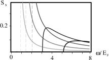
Figure 2: Spin structure factor $S_{\rm\scriptscriptstyle S}(\omega)$ in units $\hbar n_{\rm\scriptscriptstyle F}/E_{\rm\scriptscriptstyle F}$ for different scattering lengths $1/(a_{\rm\scriptscriptstyle F}k_{\rm\scriptscriptstyle F})=-0.5,-0.25,0,0.25,0.5$. The spin structure is quenched below the spin gap $\omega<\Delta_{\rm\scriptscriptstyle S}$, and exhibits a characteristic singularity in the BCS limit.

In contrast, the dynamic density structure factor $S_{\rm\scriptscriptstyle C}$ in superfluids is dominated by a collective sound excitation representing the Goldstone mode of the broken symmetry (in conventional superconductors, Coulomb interactions lift this mode to the plasma frequency). The dynamic structure factor at low momenta $k\ll 1/\xi$ takes the form

$$S_{\rm\scriptscriptstyle C}(\omega,{\bf k})=n_{\rm\scriptscriptstyle F}\frac{\hbar k}{2mc_{\rm\scriptscriptstyle s}}\delta\left(\omega-c_{\rm\scriptscriptstyle s}k\right)$$ (6)

exhausting the $f$-sum rule and compressibility sum rule,

$$\int_{0}^{\infty}d\omega\hbar\omega S_{\rm\scriptscriptstyle C}(\omega,{\bf k}) = n_{\rm\scriptscriptstyle F}\frac{\hbar^{2}{\bf k}^{2}}{2m},$$ (7)

$$\lim_{k\rightarrow 0}\int_{0}^{\infty}d\omega\frac{S_{\rm\scriptscriptstyle C}(\omega,{\bf k})}{\hbar\omega} = \frac{n_{\rm\scriptscriptstyle F}}{2mc_{s}^{2}}.$$ (8)

The determination of the sound velocity within the BEC-BCS crossover requires the calculation of the diagrams $\chi_{\rm\scriptscriptstyle coll}$ in Fig. 1; its contribution exhausts the sum rules (7) and (8) at small momenta $k\ll 1/\xi$ and frequencies $\hbar\omega<\Delta_{\rm\scriptscriptstyle S}$ i.e., a cancellation appears between $\chi_{\rm\scriptscriptstyle pair}$ and $\chi_{\rm\scriptscriptstyle coll}$ at frequencies $\omega>\Delta_{\rm\scriptscriptstyle S}$. The diagrams in $\chi_{\rm\scriptscriptstyle coll}$ provide the response function

$$\chi_{\rm\scriptscriptstyle C}(\omega,{\bf k})=4\sum_{\alpha,\beta}\phi_{\alpha}^{*}(\omega,{\bf k})\Gamma_{\alpha,\beta}(\omega,{\bf k})\phi_{\beta}(\omega,{\bf k}),$$ (9)

where one factor 2 accounts for summation of spin indices, while the second factor 2 appears as each vertex operator $\Gamma_{\alpha\beta}$ contributes to two diagrams. Using the microscopic approach by Haussmann Haussmann (1993), the vertex operator $\Gamma_{\alpha\beta}$ takes the form

$$(\Gamma_{\alpha\beta})^{-1}=\left[\frac{m}{4\pi\hbar^{2}a_{\rm\scriptscriptstyle F}}-\int\frac{d{\bf k}}{(2\pi)^{3}}\frac{m}{\hbar^{2}{\bf k}^{2}}\right]\delta_{\alpha\beta}+M_{\alpha\beta}$$ (10)

with

$$M_{pp}(\Omega_{s},{\bf k}) \!=\! T\sum_{t\in{\rm Z}}\int{\frac{d{\bf q}}{(2\pi)^{3}}}\left[\mathcal{G}(\Omega_{s-t},{\bf q\!+\!k})\mathcal{G}(\Omega_{t},-{\bf q})\right]\!,$$

$$M_{p\overline{p}}(\Omega_{s},{\bf k}) \!=\! T\sum_{t\in{\rm Z}}\int{\frac{d{\bf q}}{(2\pi)^{3}}}\left[\mathcal{F}(\Omega_{s-t},{\bf q\!+\!k})\mathcal{F}(\Omega_{t},-{\bf q})\right]\!,$$

with $M_{pp}=M_{\overline{p}\overline{p}}^{*}$ and $M_{p\overline{p}}=M_{\overline{p}p}^{*}$. The propagators $\phi^{*}_{p}$ ($\phi_{p}$) account for the creation (destruction) of a fermion pair from the condensate, and take the form

$$\phi_{p}=T\sum_{t}\int\frac{d{\bf q}}{(2\pi)^{3}}\mathcal{G}(\Omega_{t},{\bf q})\mathcal{F}(\Omega_{t+s},{\bf q+k}).$$ (11)

Solving the above equations in the limit of small frequency $\omega\ll\Delta_{\rm\scriptscriptstyle S}$ and momenta $k\ll 1/\xi$ provides the collective sound mode with sound velocity $c_{s}$; the result is shown in Fig. 3.

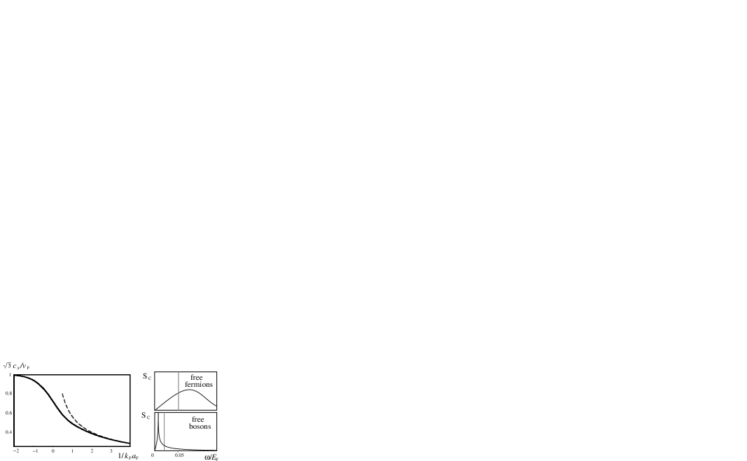
Figure 3: Left: Sound velocity $c_{s}$ in the BEC-BCS crossover in units $v_{\rm\scriptscriptstyle F}/\sqrt{3}$. The dashed line is the Bogoliubov sound velocity. Right: Structure factor $S_{\rm\scriptscriptstyle C}(\omega)$ of weakly interacting fermions and bosons above the superfluid transition temperature $T=\epsilon_{\rm\scriptscriptstyle F}/2>T_{c}$ and $k=\sqrt{3}k_{\rm\scriptscriptstyle F}/40$. The gray line denotes the peak of the sound mode below the superfluid transition.

Within the BCS limit, the collective excitations (9) provide the Bogoliubov-Anderson sound mode for a neutral superconductor with $c_{s}=v_{\rm\scriptscriptstyle F}/\sqrt{3}$ Anderson (1958). The particle-hole contributions, dominating the structure factor for a weakly interacting Fermi gas, are quenched due to the opening of the excitation gap. Note, that the leading correction to the sound velocity $c_{s}=v_{\rm\scriptscriptstyle F}/\sqrt{3}[1-8k_{\rm\scriptscriptstyle F}a_{\rm\scriptscriptstyle F}/\pi]$ derives from particle-hole scattering Anderson (1958); such scattering processes are not contained in our approach. In turn, within the BEC limit Eq. (9) gives the structure factor $S^{\rm\scriptscriptstyle BEC}_{\rm\scriptscriptstyle C}(\omega,{\bf k})=2n_{\rm\scriptscriptstyle F}\delta\big{(}\omega-\hbar{\bf k}^{2}/4m\big{)}$. The variational BCS wave function approach provides the zeroth order result describing a noninteracting Bose gas of molecules with density $n_{\rm\scriptscriptstyle B}=n_{\rm\scriptscriptstyle F}/2$ and mass $m_{\rm\scriptscriptstyle B}=m/2$. The structure factor becomes 4 times the structure factor of an ideal Bose gas. This factor 4 appears as the external potential drives the fermionic density operator instead of the bosonic density operator; the structure factor satisfies the $f$-sum rule for fermions with $n_{\rm\scriptscriptstyle F}/m=4n_{\rm\scriptscriptstyle B}/m_{\rm\scriptscriptstyle B}$. Going beyond leading order, the above equations also incorporate the repulsion between the bound pairs, and provide the structure factor $S^{\rm\scriptscriptstyle BEC}_{\rm\scriptscriptstyle C}(\omega,{\bf k})=2n_{\rm\scriptscriptstyle F}\tilde{\epsilon}_{\bf k}/\tilde{E}_{\bf k}\delta\big{(}\omega-\tilde{E}_{\bf k}/\hbar\big{)}$ with $\tilde{\epsilon}=\hbar^{2}{\bf k}^{2}/2m_{\rm\scriptscriptstyle B}$ and the Bogoliubov excitation spectrum $\tilde{E}^{2}_{\bf k}=\tilde{\epsilon}_{\bf k}^{2}+2\mu_{\rm\scriptscriptstyle B}\tilde{\epsilon}_{\bf k}$. The structure factor describes a weakly interacting Bose gas with sound velocity $c_{\rm\scriptscriptstyle s}=\sqrt{\mu_{\rm\scriptscriptstyle B}/m_{\rm\scriptscriptstyle B}}$. Here, $\mu_{\rm\scriptscriptstyle B}=4\pi\hbar^{2}a_{\rm\scriptscriptstyle B}n_{\rm\scriptscriptstyle B}/m_{\rm\scriptscriptstyle B}$ denotes the bosonic chemical potential accounting for the scattering length $a_{\rm\scriptscriptstyle B}=2a_{\rm\scriptscriptstyle F}$ within Born approximation; its exact value $a_{\rm\scriptscriptstyle B}\approx 0.6$ has recently been derived Petrov et al. (2003).

Next, we focus on the dynamic structure factor above the superfluid transition temperature $T>T_{c}$ and compare it with the structure factor Eq. (6). We first focus on the collisionless regime $\omega\tau>1$ with $\tau$ the collision time; this limit is naturally achieved for weakly interacting atomic gases ($|k_{\rm\scriptscriptstyle F}a_{\rm\scriptscriptstyle F}|<1$) and frequencies $\omega$ above the trapping frequency Pitaevskii and Stringari (2002). Within the BCS limit, the system reduces to a Fermi liquid with a weak attractive interaction. The structure factor exhibits the particle-hole excitation spectrum of a weakly interacting Fermi gas at finite temperature (interactions only renormalize the Fermi velocity $v_{\rm\scriptscriptstyle F}$), while the zero sound mode is overdamped for attractive fermions; the structure factor is shown in Fig. 3. In turn, in the BEC limit the system above the critical temperature $T_{c}$ reduces to a gas of bosonic molecules. The structure factor of a degenerate Bose gas with temperatures above the superfluid transition temperature derives from the bosonic Lindhard function; the structure at low momenta is shown in Fig. 3. Comparing these structure factors with Eq. (6), we find that the superfluid state is characterized by the appearance of a collective sound mode. However, for the system in the hydrodynamic regime $\omega\tau<1$, the structure factor is exhausted by the hydrodynamic sound mode (first sound) even above the superfluid transition. Therefore, the identification of the superfluid transition from the density response requires to be in the collisionless regime, which is reached for sufficiently weak interactions.

Within recent experiments Greiner et al. (2003); Bartenstein et al. (2004), the molecular binding energy in the BEC limit was determined by a r.f. pulse breaking the molecules and exciting a fermion into a different hyperfine state. This method has the disadvantage that the interactions between the fermions in different hyperfine states produces non-trivial energy shifts. In turn, the structure factors presented here, produce excitations within the same hyperfine states. However, the two hyperfine states are separated by an energy $\hbar\omega_{\uparrow\downarrow}$ due to Zeeman splitting. Using a driving field at frequency $\omega_{\uparrow\downarrow}$ with an additional superimposed modulation frequency $\omega$, i.e., $\lambda(t)\sim\cos(\omega_{\uparrow\downarrow}t)\cos(\omega t)$, then probes the structure factors $S_{\rm\scriptscriptstyle S}(\omega)$ with the number of particles in each hyperfine state conserved. Such a procedure avoids non-trivial energy shifts induced by a change in particle number or excitation of particles into different hyperfine state, and therefore represents a suitable setup for a determination of the two particle excitation gap $\Delta_{\rm\scriptscriptstyle S}$. The measurement of the structure factors can be achieved in two different ways: First, the energy transfer $W$ to the system satisfies $W=\gamma\omega S(\omega,{\bf k})$ with $\gamma$ determined by the driving field alone and allows for the determination of $S$ from the heating of the system Stamper-Kurn et al. (1999); Steinhauer et al. (2002). For ⁶Li, the characteristic parameters at the Feshbach resonance are given by $\Delta_{\rm\scriptscriptstyle S}\sim E_{\rm\scriptscriptstyle F}\sim 1\mu{\rm K}$ and $\omega_{\uparrow,\downarrow}\sim 80{\rm MHz}$, i.e., the structure factor is accessbile via Raman transitions or r.f. pulses as and shown in recent experiments Greiner et al. (2003); Bartenstein et al. (2004); Grimm and Chin (private discussion). Second, the interaction between the driving field and the fermions leads to the absorbtion and emission of photons with a rate determined by the structure factor $S(\omega,{\bf k})$. Therefore, an analysis of the counting statistic of the probing laser field allows for an in-situ measurement of the structure factors.