Integration of Langevin Equations with Multiplicative Noise and the Viability of Field Theories for Absorbing Phase Transitions

Abstract

Efficient and accurate integration of stochastic (partial) differential equations with multiplicative noise can be obtained through a split-step scheme, which separates the integration of the deterministic part from that of the stochastic part, the latter being performed by sampling exactly the solution of the associated Fokker-Planck equation. We demonstrate the computational power of this method by applying it to most absorbing phase transitions for which Langevin equations have been proposed. This provides precise estimates of the associated scaling exponents, clarifying the classification of these nonequilibrium problems, and confirms or refutes some existing theories.

Stochastic differential equations are ubiquitous in the description of phenomena in the natural sciences and beyond Gardiner . The coarse-graining of fast degrees of freedom often leads to effective Langevin equations where the noise term involves the mesoscopic variables of interest in a multiplicative fashion. Examples range from nonlinear quantum optics, synchronization of oscillators, or wetting phenomena, to theoretical population dynamics studies and autocatalytic chemical reactions Gardiner ; Review_MN ; Review_Haye .

An important case in nonequilibrium statistical physics is the stochastic partial differential equation governing a single, positive, concentration field $\rho=\rho({\bf r},t)$:

$${\partial_{t}}\rho({\bf r},t)=D\,\nabla^{2}\rho+a\rho-b\rho^{2}+\sigma\sqrt{\rho}\,\eta({\bf r},t),$$ (1)

where $\eta$ is a Gaussian (zero-mean) white noise (that is with correlations $\langle\eta({\bf r},t)\eta({\bf r}^{\prime},t^{\prime})\rangle=\delta({\bf r}-{\bf r}^{\prime})\delta(t-t^{\prime})$). For instance, for the reaction-diffusion process $A\to 2A$, $2A\to 0$, Eq. (1) can be obtained in a variety of ways, either from phenomelogical considerations or through more rigorous transformations Mapping . Also named “Reggeon field theory” for historical reasons, Eq. (1) describes the most prominent class of absorbing phase transitions (APT), the directed percolation (DP) class Review_Haye . Indeed, interpreted in the Itô (prepoint) sense, the unique, homogeneous $\rho=0$ solution does not evolve: it is an absorbing state. Although a wealth of models have been found to exhibit a DP transition, this class does not encompass all possible cases, and the classification of APTs is currently a very active field Review_Haye ; Review_Odor . Not only such an endeavor is of importance for conceptual reasons, but it should also yield a better understanding of the key ingredients which have impeded so far clear-cut experimental realizations of even the DP transition.

Following this line of thought, stochastic equations similar to (1) have been proposed as candidate field theories for related problems (see below). Their analyses are notoriously difficult, and mostly rely on the perturbative renormalization group machinery in the vicinity of the corresponding upper critical dimension, one of the few exceptions being a recent non-perturbative treatment of Eq. (1) in delamotte_nprg_prl03 . Given this analytical bottleneck, it is tempting, with ever-improving numerical resources, to directly integrate such stochastic equations in order to check whether they at least exhibit the universal properties they are supposed to represent. However, standard schemes either immediately run into severe difficulties. For instance, even for the zero-dimensional version of Eq. (1), a first-order explicit Euler method, viz. $\rho(t+\Delta t)=\rho(t)+\Delta t[a\rho(t)-b\rho^{2}(t)]+\sigma\sqrt{\Delta t\rho(t)}N(0,1)$, where $N(0,1)$ is a normal random variate, will ineluctably produce unphysical negative values for $\rho(t+\Delta t)$, and all the more so when $\rho\to 0$, the regime of interest for the APT. Another route, which would first trade the square-root noise for a less singular one through some change of variables (e.g., $\rho\to\psi^{2}$, or a Cole-Hopf transformation $\rho\to e^{\pm 2\phi}$), is also numerically unbearable since it generates pathological deterministic terms as the original variable $\rho\to 0$. Faced with this problem in the same context, Dickman proposed Dickman_scheme , somewhat ironically, to also discretize $\rho$, yielding a scheme consistent to the order ${\cal{O}}(\sqrt{\Delta t})$ in the limit $\Delta t\to 0$. This approach has been used with some success Dickman_scheme ; Munoz_pdemany97 ; Munozetal_fes_num , but one can legitimately wonder to what extent one is truly simulating the original, continuous equation. In this respect, that the associated results are affected by the same long transients as those observed in microscopic models is also worrisome.

In this Letter, elaborating upon a method pioneered by Pechenik and Levine in the somewhat distant context of front selection mechanisms in microscopic reaction-diffusion models PL , we overcome the above hurdles. We first demonstrate the power of this approach on Eq. (1) before applying it to most related APTs for which a Langevin equation has been proposed, including the voter critical point with its two symmetric absorbing states Voter_dickman ; Voter_us . Our results are particularly worthy in the context of the current debate about APTs occurring when $\rho$ is coupled to an auxiliary field $\psi$: when $\psi$ is static and conserved (Manna sandpile model, conserved-DP, or fixed energy sandpiles class) FvW ; Alexv_PRL ; Alexv_PRE ; Fes_PRL ; Munozetal_fes_num ; JK_HC_PRL2 we obtain the best numerical estimates for the critical indices. When $\psi$ is conserved but diffuses KSS ; WOH ; WOH_JSP ; Freitas00 ; Janssen01 ; Freitas01 ; Janssen04 , our results suggest that, at least in low spatial dimensions, the Langevin equations postulated or derived (approximately) as candidate field theories are not viable.

The idea underlying the approach of PL (of which we become aware while this paper was upon completion) is a general and rather natural one, since it consists in integrating the fast degrees of freedom. An Itô stochastic differential equation of the form $\frac{{\rm d}\rho}{{\rm d}t}=f(\rho)+\sigma g(\rho)\eta(t)$ is dealt with the so-called operator-splitting scheme: the stochastic part $\sigma g(\rho)\eta(t)$ is integrated first, not by using a Gaussian random number, but by directly sampling the time-dependent solution of the associated Fokker-Planck equation (FPE). Namely, one generates a random number $\rho^{*}$ distributed according to the conditional transition probability density function (p.d.f.) ${\rm Proba.}\{\rho(t+\Delta t)=\rho^{*}|\rho(t)=\rho_{0}\}$, and then use $\rho^{*}$ for evolving the deterministic part $f(\rho)$ with any standard numerical method for ordinary differential equations. Since the integration of the stochastic part is accomplished through the exact solution of the FPE, which is first-order in time, the overall precision of the scheme, ${\cal{O}}(\Delta t)$, is already significantly superior to that of a naive Euler method (anyhow flawed for Eq.(1)), or to Dickman’s approach.

Now, for the square-root noise case, i.e., $g(\rho)\equiv\sqrt{\rho}$, the closed form solution $P(\rho,t)={\rm Proba.}\{\rho(t)=\rho|\rho(0)=\rho_{0}\}$ of the associated FPE $\partial_{t}P(\rho,t)=\frac{\sigma^{2}}{2}\partial^{2}_{\rho}[\rho P(\rho,t)]$, has been known in the mathematical literature for more than half a century Feller (see also PL ):

$$P(\rho,t)=\delta(\rho)e^{-\frac{2\rho_{0}}{\sigma^{2}t}}+\frac{2e^{-\frac{2(\rho_{0}+\rho)}{\sigma^{2}t}}}{\sigma^{2}t}\sqrt{\frac{\rho_{0}}{\rho}}I_{1}\left(\frac{4\sqrt{\rho_{0}\rho}}{\sigma^{2}t}\right),$$ (2)

($I_{1}$ is the modified Bessel function of the first kind of order 1). When, further, the deterministic part is linear, i.e. $f(\rho)=\alpha+\beta\rho$, with $\alpha>0$, the exact conditional transition p.d.f. of the full equation $\frac{{\rm d}\rho}{{\rm d}t}=\alpha+\beta\rho+\sigma\sqrt{\rho}\eta$ has also been determined Feller :

$$P(\rho,t)=\lambda e^{-\lambda(\rho_{0}e^{\beta t}+\rho)}\left[\frac{\rho}{\rho_{0}e^{\beta t}}\right]^{\frac{\mu}{2}}I_{\mu}\left(2\lambda\sqrt{\rho_{0}\rho e^{\beta t}}\right),$$ (3)

($I_{\mu}$ being a Bessel function of order $\mu$) where, to condense notations, we have set $\lambda=\frac{2\beta}{\sigma^{2}(e^{\beta t}-1)}$, and $\mu=-1+\frac{2\alpha}{\sigma^{2}}$.

The scheme we have used to integrate Eq.(1) and its siblings relies on the latter results. After discretizing the Laplacian $\nabla^{2}\rho$ over the $2d$ nearest-neighbors ${\bf r}+{\bf e}_{v}$ of site ${\bf r}$ on a $d$-dimensional hypercubic lattice of mesh size $\Delta x$, we first sample, between $t$ and $t+\Delta t$, the solution of the FPE associated to each local linear equation $\frac{{\rm d}\rho}{{\rm d}t}=\alpha+\beta\rho+\sigma\sqrt{\rho}\eta$ using Eq.(6) with $\beta=a-\frac{2dD}{(\Delta x)^{2}}$ and

$$\alpha=\alpha({\bf r},t)=\frac{D}{(\Delta x)^{2}}\sum_{v=1}^{2d}\rho({\bf r}+{\bf e}_{v},t).$$ (4)

The value $\rho^{*}$ coming from the stochastic sampling step is, by construction, automatically non-negative, and serves as the initial condition for the remaining part of Eq.(1), i.e. $\partial_{t}\rho({\bf r},t)=-b\rho^{2}({\bf r},t)$, which can be trivially integrated to yield $\rho({\bf r},t+\Delta t)=\frac{\rho^{*}}{1+\rho^{*}b\Delta t}$. Given that $b>0$, the non-negativity of $\rho({\bf r},t)$ will be preserved at all times if, initially, $\rho({\bf r})\geq 0$ everywhere, since $\alpha$ given by Eq.(4) will also be non-negative and Eq.(6) can be used.

It remains to sample the above p.d.f., Eq.(2) or Eq.(3). Instead of using a table method, as the authors of PL , we remark that, with the help of the Taylor-series expansion of the Bessel function, Eq.(3) can be rewritten as

$$P(\rho,t)=\sum_{n=0}^{\infty}\frac{\left(\lambda\rho_{0}e^{\beta t}\right)^{n}e^{-\lambda\rho_{0}e^{\beta t}}}{n!}\frac{\lambda e^{-\lambda\rho}(\lambda\rho)^{n+\mu}}{\Gamma(n+\mu+1)}.$$ (5)

In other words, one has the following mixture Devroye :

$$\rho^{*}={\rm Gamma}[\mu+1+{\rm Poisson}[\lambda\rho_{0}e^{\beta t}]]/\lambda,$$ (6)

where ${\rm Prob.}\{{\rm Poisson}[\lambda\rho_{0}e^{\beta t}]=n\}=\frac{\left(\lambda\rho_{0}e^{\beta t}\right)^{n}e^{-\lambda\rho_{0}e^{\beta t}}}{n!}$, and ${\rm Prob.}\{{\rm Gamma}[\omega]=v\}=\frac{e^{-v}v^{\omega-1}}{\Gamma(\omega)}$. This procedure will reconstitute, on average, all the terms of Eq.(5) with their correct probability, and gives us — since standard and uniformly fast generators of Poisson and Gamma random numbers are available — a means of sampling in a “numerically exact” way these p.d.f. NOTE .

Typical results for Eq.(1) in one dimension are shown in Fig. 1, along with data obtained using Dickman’s method. Except for the (weak) linear stability requirement coming from the discretized Laplacian, there is no limitation on $\Delta t$ with the former method, so that the computational gain is of several orders of magnitude, together with an unusually clean algebraic decay of $\langle\rho\rangle$, with an exponent $\theta=0.1595(2)$ matching to the fourth decimal the series-expansion result Review_Haye ; Review_Odor . In fact, even if $\Delta t=0.25$ for this run, the threshold $a=a_{c}(\Delta t)$ is within one percent off its extrapolated limit value as $\Delta t\to 0$, suggesting that the continuous limit of Eq.(1) is already resolved. One of the reasons for the particular efficiency of this scheme even with such a large timestep is that it automatically takes into account, and in a self-adaptive fashion through the locally varying value of $\alpha$ (Eq.(4)), the strongly non-Gaussian modifications undergone by the instantaneous, conditional p.d.f., Eq.(2) or Eq.(3), as one gets closer and closer to the absorbing barrier.

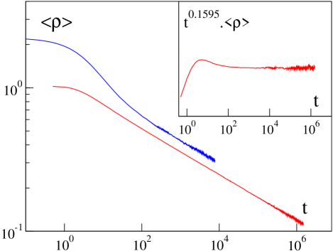
Figure 1: (Color online) Density decay $\langle\rho\rangle=\langle\rho({\bf r},t)\rangle_{\bf r}\sim t^{-\theta}$ at criticality for Eq.(1) in $d=1$. Lower curve: using our scheme ($\Delta t=0.25$, $\Delta x=1$, $a=a_{\rm c}=1.75623(2)$, $b=1$, $D=0.25$, $\sigma^{2}=2$, single run for a system of $2^{22}$ sites with $\rho=1$ everywhere initially); a least-square fit gives $\theta=0.1595(2)$. Upper curve: using Dickman’s method (similar conditions, but $\Delta t=10^{-3}$). Inset: Plateau of the local exponent.

We now present some of our most salient results obtained for Langevin equations similar to (1), deferring a more detailed account of our investigations to TBP .

DP coupled to a non-conserved, non-diffusing field. To account for reaction-diffusion processes such as $2A\to 3A$, $2A\to A$ where single particles do not move (such as the prototypical pair-contact process PCP ) and which thus possess infinitely-many absorbing states, it has been proposed that Eq.(1) be supplemented by the non-Markovian term $c\exp[-w\int_{0}^{t}{\rm d}s\,\rho({\bf r},s)]$ to account for the memory effect introduced by immobile particles DP_manyabs . The impact of this term is however unclear, with early simulations Munoz_pdemany97 using Dickman’s method suggesting that continuously-varying spreading exponents arise, in agreement with results obtained on microscopic models PCP , but in contradiction with the study of infinite-memory spreading processes inf_mem , which support stretched-exponential behavior. Simulations with our scheme, in one dimension, reveal power-laws for small $|c|$, but curvature appears at late times for large, negative $c$ values (Fig. 2a). To be fully conclusive, these results will have to be improved by using enrichment methods enabling to explore rare events, but they already indicate that the conclusions of inf_mem probably hold asymptotically. We finally mention that in two dimensions (and for $c>0$, $b=0$) we obtain dynamical percolation spreading exponents as predicted by the standard theory DP_manyabs .

DP coupled to a conserved, non-diffusing field. Reaction processes such as $A+B\to 2A$, $A\to B$ where $A$ particles diffuse and $B$ are static, are similar to the case above, but the number of particles is (locally) conserved Alexv_PRL . This conservation law leads to couple $\rho$ to a conserved field $\phi$ in the following system Alexv_PRE ; Fes_PRL :

$$\begin{array}[]{lll}\partial_{t}\rho&=&D\,\nabla^{2}\rho+a\rho-b\rho^{2}+\omega\rho\phi+\sigma\sqrt{\rho}\,\eta({\bf r},t)\\ \partial_{t}\phi&=&D_{\rho}\,\nabla^{2}\rho\end{array}$$ (7)

Microscopic models leading to (7) also include so-called fixed energy sandpiles such as the Manna model, establishing a link between APTs and self-organized criticality Fes_PRL . The conservation law influences even the static exponents but definite estimates are currently not available (see Munozetal_fes_num and references therein). Data from microscopic models, as well as simulations of (7) using Dickman’s method are plagued by long transients/corrections to scaling. Our scheme leads, again, to clean power-laws which provide us with the best estimates for the scaling exponents of this class of APT. In Fig. 2b, we show a typical result for critical decay in $d=1$, leading to $\theta=0.125(2)$, unambiguously distinct from the DP value 0.1595(1). Critical decay exponents obtained in higher dimensions, $\theta_{2d}=0.509(5)$ and $\theta_{3d}=0.81(1)$ TBP , differ also significantly from their DP counterparts.

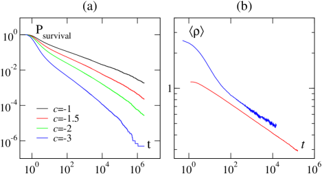
Figure 2: (Color online) (a): Survival probability of an initial seed at ${\bf r}={\bf 0}$ evolving under Eq.(1) with the extra term $c\exp[-w\int_{0}^{t}{\rm d}s\,\rho({\bf r},s)]$. Same parameters as in Fig. 1 and various $c$ values (about $10^{7}$ trials). (b): Same as Fig. 1 but for Eqs.(7). Lower curve: with our scheme ($\Delta t=0.1$, $\Delta x=1$, $a=a_{\rm c}=0.86455(5)$, $b=\omega=1$, $D=D_{\rho}=0.25$, $\sigma^{2}=2$, $\rho=\phi=1$ everywhere initially); A least-square fit gives $\theta=0.124(1)$. Upper curve: with Dickman’s method ($\Delta t=0.0025$).

DP coupled to a conserved, diffusing field. If, for the reaction processes above, both species are diffusing, the situation changes again, if only because one has now a single, dynamic absorbing state (where $B$ particles diffuse in the absence of $A$s). This case was studied both analytically KSS ; WOH ; WOH_JSP ; Janssen01 ; Janssen04 and numerically Freitas00 ; Freitas01 with continuous APT predicted and observed for $0<D_{\phi}\leq D$, but with conflicting estimates of scaling exponents Janssen01 ; Freitas01 . The corresponding Langevin equation is usually cast WOH_JSP ; Janssen04 as Eqs.(7) complemented by the self-diffusion of the auxiliary field and a conserved noise term. Performing with our scheme critical decay experiments in spatial dimensions $d=1,2$ we find the exponent $\theta$ to be undistinguishable from the DP values. Because this differs from both analytical predictions KSS ; WOH ; Janssen01 and estimates from microscopic models Freitas01 , this indicates that the truncation of the full action of the field theory needed to arrive at the corresponding Langevin equations is not legitimate.

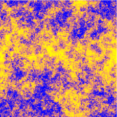
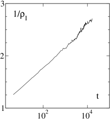
Figure 3: (Color online) Voter coarsening process for a continuous field evolving under Eq.(8) ($\Delta x=1$, $\Delta t=0.25$, $D=1$, $\sigma^{2}=0.5$, zero-mean random initial conditions) Left: snapshot of $\rho$ at $t=2500$ ($512^{2}$ sites). Right: decay of interface density ($4096^{2}$ sites) $\rho_{I}=1-\langle\rho({\bf r},t)\rho({\bf r}+{\bf e}_{v},t)\rangle\propto 1/\ln t$.

The voter critical point. The universality class of the voter model is characterized by two symmetric absorbing states Voter_us . The following field theory has been proposed —but never tested— to describe its critical point Voter_dickman ; Janssen04 :

$$\partial_{t}\rho=D\,\nabla^{2}\rho+\sigma\sqrt{1-\rho^{2}}\,\eta({\bf r},t)$$ (8)

The FPE associated to the sole stochastic part can be solved through an eigenfunction expansion, leading to a complicated expression for the conditional transition p.d.f., involving a continuous part and two delta peaks at the barriers $\rho=\pm 1$ PL ; TBP . Although this distribution can be sampled TBP , it is both much simpler and more efficient to replace in the noise term the piece $\sqrt{1-\rho^{2}}$ by $\Theta(\rho)\sqrt{1-\rho}+(\rho\leftrightarrow-\rho)$, thereby taking into account just the closest DP barrier. This way our scheme can be applied and, one observes in two dimensions phase ordering patterns typical of the marginal voter coarsening process, and, for the first time with continuous variables, the expected $1/\ln t$ decay of the density of interfaces (Fig. 3).

This completes our (not-exhaustive) inspection of Langevin equations proposed as field theories of absorbing phase transitions. Pending more comprehensive studies (higher dimensions, other scaling exponents), the results already obtained demonstrate that the method presented above enables faithful and efficient simulations of such stochastic equations. This approach will remain particularly useful as long as no major analytical progress is made, and also to test future theoretical predictions.

M. A. M. acknowledges financial support from the Spanish MCyT (FEDER) under project BFM2001-2841.

References

- (1) W.C. Gardiner, Handbook of Stochastic Methods for Physics, Chemistry and the Natural Sciences (Springer, 3rd edition, 2004).
- (2) M. A. Muñoz, in Advances in Condensed Matter and Statistical Mechanics, E. Korutcheva and R. Cuerno eds. (Nova Science Publ., 2003), and references therein.
- (3) H. Hinrichsen, Adv. Phys. 49, 815 (2000).
- (4) G. Ódor, Rev. Mod. Phys. 76, 663 (2004).
- (5) M. Doi, J. Phys. A 9, 1479 (1976); P. Grassberger and M. Scheunert, Fortschr. Phys. 28, 547 (1980); L. Peliti, J. Phys. (Paris) 46, 1469 (1984);
- (6) L. Canet et al., Phys. Rev. Lett. 92, 195703 (2004).
- (7) R. Dickman, Phys. Rev. E 50, 4404 (1994).
- (8) C. López and M.A. Muñoz, Phys. Rev. E 56, 4864 (1997).
- (9) J. J. Ramasco, M. A. Muñoz, and C. A. da Silva Santos, Phys. Rev. E 69, 045105 (2004).
- (10) L. Pechenik and H. Levine, Phys. Rev. E 59, 3893 (1999).
- (11) R. Dickman and A. Yu. Tretyakov, Phys. Rev. E 52, 3218 (1995).
- (12) I. Dornic et al., Phys. Rev. Lett. 87, 045701 (2001).
- (13) F. van Wijland, Phys. Rev. Lett. 89, 190602 (2002); Braz. J. Phys. 33, 551 (2003).
- (14) M. Rossi, R. Pastor-Satorras, and A. Vespignani, Phys. Rev. Lett. 85, 1803 (2000).
- (15) R. Pastor-Satorras and A. Vespignani, Phys. Rev. E 62, R5875 (2000).
- (16) A. Vespignani et al., Phys. Rev. Lett. 81, 5676 (1998). R. Dickman, et al., Braz. J. of Phys. 30, 27 (2000).
- (17) J. Kockelkoren and H. Chaté, cond-mat/0306039.
- (18) R. Kree, B. Schaub, and B. Schmittmann, Phys. Rev. A 39, 2214 (1989).
- (19) F. van Wijland, K. Oerding, and H. J. Hilhorst, Physica A 251, 179 (1998).
- (20) K. Oerding et al., J. Stat. Phys. 99, 1365 (2000).
- (21) H. K. Janssen, cond-mat/0304631v2.
- (22) J. E. de Freitas et al., Phys. Rev. E 61, 6330 (2000).
- (23) H.-K. Janssen, Phys. Rev. E 64, 058101 (2001).
- (24) J. E. de Freitas et al., Phys. Rev. E 64, 058102 (2001).
- (25) W. Feller, Ann. Math. 54, 173 (1951).
- (26) L. Devroye, Non-Uniform Random Variate Generation, Springer (New York), 1986.
- (27) By continuity, Eq.(6) can also be used to sample Eq.(2), with the (natural) convention .
- (28) I. Dornic, H. Chaté, and M. A. Muñoz, in preparation.
- (29) I. Jensen, Phys. Rev. Lett. 70, 1465 (1993).
- (30) M. A. Muñoz et al., Phys. Rev. Lett. 76, 451 (1996); M. A. Muñoz, G. Grinstein, and R. Dickman, J. Stat. Phys. 91, 541 (1998).
- (31) P. Grassberger, H. Chaté, and G. Rousseau, Phys. Rev. E 55, 2488 (1997); A. Jiménez-Dalmaroni and H. Hinrichsen, Phys. Rev. E 68, 036103 (2003).