The American put and European options near expiry, under Lévy processes

Abstract.

We derive explicit formulas for time decay, $\theta$, for the European call and put options at expiry, and use them to calculate analytical approximations to the price of the American put and early exercise boundary near expiry. We show that for many families of non-Gaussian processes used in empirical studies of financial markets, the early exercise boundary for the American put without dividends is separated from the strike price by a non-vanishing margin on the interval $[0,T)$. As the riskless rate vanishes and the drift decreases accordingly so that the stock remains a martingale, the optimal exercise price goes to zero uniformly over the interval $[0,T)$. The implications for parameters’ fitting are discussed.

Department of Economics, The University of Texas at Austin, 1 University Station C3100, Austin, TX 78712-0301, U.S.A. (e-mail: leven@eco.utexas.edu)

Key words: Lévy processes, early exercise boundary

JEL Classification:  D81, C61

Mathematics Subject Classification (1991):  90A09, 60H30, 60G44

1 Introduction

By now, jump-diffusion processes and more general Lévy processes or Lévy driven processes are widely used in models of the stock dynamics and term structure models, under both historic and risk neutral measure. However, only discrete time series of empirical data are available, therefore the problem of identification of the jump and diffusion components is a non-trivial task. The problem of the identification of the diffusion component was considered in detail in Aıt-Sahalia (2002, 2003); in the present paper, the focus is on the jump component. Clearly, the presence of jumps is most prominent in prices of contingent claims near expiry, especially for out-of-the money options, and therefore it is natural to extract information about the jump part of the process by using empirical data for out-of-the-money European options. Carr and Wu (2003) showed that in the presence of jumps, the prices of out-of-the-money European options near expiry are of order $\tau$, where $\tau$ is the time to expiry, and use this observation to test for the presence of jumps. However, the results in Carr and Wu (2003) are qualitative rather than quantitative.

The principal aim of the present paper is to derive simple analytical formulas which can be used for the identification of the jump part of a Lévy process (under a risk-neutral measure chosen by the market); the straightforward generalizations to mean-reverting processes driven by Lévy processes (the Ornstein-Uhlenbeck type processes), stochastic volatility models with jumps and Lévy-driven term structure models will be published elsewhere. The first group of results of the present paper are formulas for $\theta$, or time decay, of out-of-the money European call and put options on a stock, at expiry. Contrary to the Gaussian case, $\theta$ for the former (resp., the latter) is shown to be negative if there are positive (resp., negative) jumps. In other words, we prove that near expiry, these prices are linear functions of time to expiry (up to relatively small errors), and calculate the coefficients. The results are explicit analytical expressions in terms of the parameters which characterize the process. By using these formulas and empirical data for options near expiry as in Carr and Wu (2003), it is possible to identify the jump part of a particular Lévy model. After that, by using the data for options far from expiry, one can identify the first instantaneous moment of the process, and calculate the diffusion coefficient by subtracting the second instantaneous moment of the jump part of the process. This gives a new identification method for the diffusion component.

By using the formulas for the $\theta$’s for the European put and call, we obtain approximations for the American put price and early exercise boundary near expiry. The pricing of American options in the Gaussian case is well understood – see e.g. Musiela and Rutkowski (1997), Karatzas and Shreve (1998), Carr and Faguet (1994), Carr (1998), Longstaff and Schwartz (2001), Clément et al. (2002), and the bibliography therein. In the infinite horizon case, explicit analytical formulas are obtained, and in the finite horizon case, a number of efficient numerical methods are developed. Although explicit formulas are not available in the finite horizon case, several general results are proved for this case as well. Consider the American put with the strike price $K$ and maturity $T$, on a non-dividend paying stock; the riskless rate $r>0$ is constant. Let $H(t)=H(r,K,T;t)$ be the optimal exercise price of the American put. If the stock log-price $X_{t}=\log S_{t}$ follows the Brownian motion, then the asymptotic behavior of $H(r,K,T;t)$ is known both near expiry:

$$\log(H(r,K,T;t)/K)\sim-\sigma\sqrt{(t-T)\ln(T-t)},$$ (1.1)

as $t\to T-0$ (see, e.g., Barles et al. (1995) and Lamberton (1995); an asymptotic formula for the put price is also available), and for small values of $r$: for any $t<T$,

$$H(r,K,T;t)\to 0,\quad{\rm as}\ r\to+0$$ (1.2)

(see, e.g. Musiela and Rutkowski (1997); (1.2) is formulated as follows: if the riskless interest rate is zero, then the early exercise of the American put is not optimal). Notice that (1.1) implies that

$$\lim_{t\to T}H(r,K,T;t)=K,$$ (1.3)

and that (1.3) and (1.2) do not agree well when both the riskless interest rate and time to expiry vanish.

In Levendorskiǐ (2003), a variant of Carr’s randomization method was developed for wide families of Lévy processes, and as a by-product, it was shown that for many families of non-Gaussian processes used in empirical studies of financial markets, the analogs of (1.3) and (1.2) agree much better. Namely,

$$\lim_{t\to T}H(r,K,T;t)=H_{T}(r,K),$$ (1.4)

where $H_{T}(r,K)$ depends on some of parameters which characterize the price process, and is smaller than the strike price, $K$. Moreover, it was proved that $H_{T}(r,K)$ vanishes with $r$, and therefore,

$$H(r,K,T;t)\to 0,\quad{\rm as}\ r\to 0,\hskip 5.69046ptuniformly\ in\hskip 5.69046ptt\in[0,T).$$ (1.5)

Notice that (1.5) looks more natural than (1.2), and may be of some importance in today’s almost deflationary world. Further, if the difference $K-H_{T}(r,K)$ is sizable, then any numerical procedure or parameters’ fitting procedure which does not take this fact into account, may produce significant errors near expiry and strike. Hence, the non-standard behavior of the early exercise boundary has practical implications for the parameters’ fitting and development of accurate numerical methods.

However, the proof in Levendorskiǐ (2003) has three disadvantages, which stem from the use of the Wiener-Hopf method. First, the non-standard behavior of the early exercise boundary results from long calculations without clear intuition. Next, the approximate formulas for the put price are expressed in terms of the factors in the Wiener-Hopf factorization formula, hence, they are complicated for practical use, and finally, the method in Levendorskiǐ (2003) is not directly applicable to a popular class of Variance Gamma Processes, which was used in Carr et al (2002), Madan and Hirsa (2003), and Carr and Hirsa (2003) for pricing of American put. The generalization of the method for more general classes of processes seems impossible.

Here we prove (1.4) and (1.5) by using a much simpler argument. We obtain an efficient approximation for the put price near expiry, and formulate the result about the non-standard behavior of the early exercise boundary in a more meaningful form. Also, we extend the result in Levendorskiǐ (2003) to Variance Gamma Processes, and in addition, we find a condition on a process which ensures that the behavior of the boundary is even more regular than in the Gaussian case: there exists a negative constant $h^{0}$ s.t.

$$H(r,K,T;t)-K\sim h^{0}\cdot(T-t)<0,\quad{\rm as}\ t\to T.$$ (1.6)

We prove that the limit of the boundary at expiry is located where $-\theta$ of the European call is equal to the riskless rate. (If the $-\theta$ of the European call at expiry is less than the riskless rate for all spot prices less than the strike, then the limit is the strike.) When the corresponding equation is solved, one can use the formulas for $\theta$’s of the European call and put and obtain an efficient approximation to the put price near expiry. The formulas are fairly simple and can be used for parameters’ fitting purposes near expiry, both for the European options and American put. They also can be used to improve performance of numerical methods: when using the backward induction, one can start not at expiry, where the value function is most irregular but close to it, and use the analytical approximation as the basis for the backward induction.

We demonstrate how large the deviations from the standard behavior of the early exercise boundary and put price can be by using the empirical data for the American put documented in Carr et al. (2002). We found that the non-standard behavior should be observed for reasonable values of the riskless rate: typically, the margin between the strike and boundary is 10% or more, and for the spot price in the 5%–interval around the strike, the “jump premium” in the put price over the pay-off is $0.5\tau$ or more, where $\tau$ is the time to expiry (with the normalization $\tau=1$ for a business year).

The last aim of the paper is to describe the restrictions on the log-price process under an EMM, which should be satisfied if the non-standard behavior of the early exercise boundary is observed. As (1.3), (1.4) and (1.6) imply, various types of the behavior of $H(r,K,T;t)$ near expiry are possible. However, for many families of processes used in empirical studies of financial markets, namely, Hyperbolic Processes, Normal Inverse Gaussian processes (NIG), and Truncated Lévy Processes of the extended Koponen’s family (a.k.a. KoBoL processes, a.k.a. CGMY model) of order $\nu\in(1,2)$, the behavior of the early exercise boundary is non-standard for all parameters’ values. This means that if in the empirical studies, the early exercise boundary for put options on a particular stock exhibits the standard behavior near expiry, then the use of any of the processes above to model the log-price dynamics under a risk-neutral measure chosen by the market is inconsistent with the data. Normal Inverse Gaussian processes, Hyperbolic Processes and KoBoL processes of order greater than 1 are processes with sample paths of infinite variation. Notice that the non-standard behavior of the early exercise boundary is proved for much wider classes of infinite variation Lévy processes as well. For processes with finite variation jump component, the prominent examples being Variance Gamma Processes and KoBoL processes of order less than 1, both the non-standard behavior (1.4) and “super-regular” behavior (1.6) of the early exercise boundary are possible, depending on parameters of the process; there are also borderline cases, when we are able only to prove that (1.3) holds. According to a recent empirical study in Carr et al. (2002), finite variation processes fit empirical data better.

Even for a finite variation process, if we fix all the parameters of a process except for the drift $\mu$, let $r\to 0$ and change $\mu$ accordingly so that the stock remains a martingale, then below a certain critical value of $r$ (depending on the parameters of the process), the non-standard behavior is observed, and as $r$ decreases further, the optimal exercise price goes to zero uniformly over the interval $[0,T)$.

It is natural to ask how robust the result about the non-standard behavior of the early exercise boundary is. In Levendorskiǐ (2003) and the present paper, it is assumed that dynamics of log-prices $X_{t}=\log S_{t}$ follows a non-Gaussian Lévy process under a risk-neutral measure chosen by the market. This simplest choice of a non-Gaussian risk-neutral measure for pricing of the American put was employed in Carr et al (2002), Madan and Hirsa (2003), Carr and Hirsa (2003), where parameters’ fitting and computational issues where addressed. Better fit can be achieved with stochastic volatility models with jumps but the method in Levendorskiǐ (2003) cannot be generalized for stochastic volatility models. The method of the present paper can be applied to stochastic volatility models (and term structure models), and under certain parameter restrictions, the margin between the early exercise boundary and strike can be derived. Further, in Levendorskiǐ (2003) and the present paper, the formulas for the margin are derived in two different approximate models, and in cases which were considered in the both papers, the formulas for the margin are the same. The identical results in two approximations allows one to hope that the margin in the continuous time model is the same. As a proven theorem, we can only claim that the margin in the approximate model is not less than in the continuous time model.

The rest of the paper is organized as follows. In Section 2, we recall the definition of Lévy processes, and give examples of several families of Lévy processes used in empirical studies of financial markets. In Section 3, $\theta$’s of out-of-the-money European put and call options are calculated, and in Section 4, the approximate formulas for the American put price and early exercise boundary near expiry are derived. In Section 5, we consider several families of Lévy processes used (and suggested for use) in empirical studies of financial markets, and discuss the implications of non-standard behavior of prices and early exercise boundary for the choice of a family of processes, and parameters’ fitting in more detail. In Section 6, we derive properties of the early exercise boundary for KoBoL processes, for parameters’ values documented in Carr et al. (2002), and show that the margin between the strike price and early exercise boundary can be significant indeed: more than 10%. In the appendix, the technical proofs are given.

2 Lévy processes

Recall that a Lévy process is a process with stationary independent increments (for general definitions, see e.g. Sato (1999)). A Lévy process may have a Gaussian component and/or pure jump component. The latter is characterized by the density of jumps, which is called the Lévy density. We denote it by $F(dx)$. Also, a Lévy process can be completely specified by its characteristic exponent, $\psi$, definable from the equality $E\left[e^{i\xi X(t)}\right]=e^{-t\psi(\xi)}$ (we confine ourselves to the one-dimensional case). If $X_{t}$ is a Lévy process with finite variation jump component, then the characteristic exponent is given by

$$\psi(\xi)=-i\mu\xi+\frac{\sigma^{2}}{2}\xi^{2}+\int_{-\infty}^{+\infty}(1-e^{i\xi y})F(dy),$$ (2.1)

where $\sigma^{2}$ and $\mu$ are the variance and drift coefficient of the Gaussian component, and $F(dy)$ satisfies

$$\int_{{\bf R}\setminus\{0\}}\min\{1,|y|\}F(dy)<+\infty.$$

Equation (2.1) is a special case of the Lévy-Khintchine formula; for the general case, see e.g. Sato (1999).

Wide families of jump-diffusion processes used in the theoretical and empirical studies of financial markets are Lévy processes with finite variation jump component.

Example 2.1. Let $X$ be a Lévy process with the Lévy density

$$F(dx)=c_{+}{\lambda_{+}}e^{{\lambda_{+}}x}{\bf 1}_{(-\infty,0)}(x)dx+c_{-}(-{\lambda_{-}})e^{{\lambda_{-}}x}{\bf 1}_{(0,+\infty)}(x)dx,$$ (2.2)

where ${\lambda_{+}}>0>{\lambda_{-}}$, and $c_{\pm}>0$. Then

$$\psi(\xi)=\frac{\sigma^{2}}{2}\xi^{2}-i\mu\xi+\frac{ic_{+}\xi}{{\lambda_{+}}+i\xi}+\frac{ic_{-}\xi}{{\lambda_{-}}+i\xi},$$ (2.3)

where $\sigma^{2}>0$ and $\mu\in{\bf R}$ are the variance and drift of the Gaussian component. The $\psi(\xi)$ is holomorphic in the strip $\Im\xi\in({\lambda_{-}},{\lambda_{+}})$. In order that $E[e^{X_{t}}]$ be finite, we need to impose an additional condition ${\lambda_{-}}<-1$. For the sake of brevity, we will consider below the exponential jump-diffusions with the characteristic exponent of the form (2.3). The generalization to the case of Lévy densities given by general exponential polynomials on positive and negative half-axis is straightforward.

Example 2.2. Variance Gamma Processes (VGP) have been developed and used by Madan and co-authors in a series of papers during 90th (see Madan et al. (1998) and the bibliography there). The characteristic exponent of a VGP without the diffusion component can be represented in the form

$$\psi(\xi)=-i\mu\xi+c[\ln({\lambda_{+}}+i\xi)-\ln{\lambda_{+}}+\ln(-{\lambda_{-}}-i\xi)-\ln(-{\lambda_{-}})],$$ (2.4)

where ${\lambda_{+}}>0>{\lambda_{-}},c>0$ and $\mu\in{\bf R}$. The condition $E[e^{X_{t}}]<+\infty$ imposes an additional restriction ${\lambda_{-}}<-1$.

Example 2.3. Truncated Lévy Processes (TLP) constructed by Koponen (1995) were used for modeling in real financial markets in Bouchaud and Potters (1997), Cont et al. (1997) and Matacz (2000); a generalization of this family was constructed in Boyarchenko and Levendorskiǐ (1999, 2000) and called the extended Koponen family of TLP processes. Later, this generalization was used in Carr et al. (2002) under the name CGMY-model. As A.N. Shiryaev remarked, the name TLP was misleading, and so starting with Boyarchenko and Levendorskiǐ (2002a-2002c), we use the name KoBoL processes.

The characteristic exponent of a KoBoL process is of the form

$$\psi(\xi)=-i\mu\xi+c\Gamma(-\nu)[{\lambda_{+}}^{\nu}-({\lambda_{+}}+i\xi)^{\nu}+(-{\lambda_{-}})^{\nu}-(-{\lambda_{-}}-i\xi)^{\nu}],$$ (2.5)

where $\nu\in(0,2),\nu\neq 1,c>0,{\lambda_{-}}<0<{\lambda_{+}}$, and $\mu\in{\bf R}$. The condition $E[e^{X_{t}}]<+\infty$ imposes an additional restriction ${\lambda_{-}}\leq-1$. (In Boyarchenko and Levendorskiǐ (1999, 2000, 2002b), the reader can also find a formula for the KoBoL process of order $\nu=1$).

For $\nu\in(0,1)$, the equation (2.5) is obtained from (2.1) with the Lévy density given by

$$F(dx)=c{\lambda_{+}}e^{{\lambda_{+}}x}{\bf 1}_{(-\infty,0)}(x)|x|^{-\nu-1}dx+c(-{\lambda_{-}})e^{{\lambda_{-}}x}{\bf 1}_{(0,+\infty)}(x)x^{-\nu-1}dx,$$ (2.6)

and $\sigma=0$ (that is, there is no Gaussian component). In the case $\nu\in(1,2)$, instead of (2.1), the general form of the Lévy-Khintchine formula is needed (see Sato (1999) and Boyarchenko and Levendorskiǐ (2002b)). KoBoL processes of order $\nu\in(0,1)$ are finite-variation processes, and the ones of order $\nu\in(1,2)$ are infinite-variation processes.

Other examples of infinite variation processes are Hyperbolic Processes (HP), Normal Inverse Gaussian processes (NIG) and Normal Tempered Stable (NTS) Lévy processes of order $\nu\in(1,2)$; in the general classification of Boyarchenko and Levendorskiǐ (1999, 2000, 2002a-2002c), HP and NIG are processes of order 1. Hyperbolic Processes were constructed and used by Eberlein and co-authors (see e.g. Eberlein and Keller (1995), Eberlein et al. (1998), Eberlein and Raible (1999)); hyperbolic distributions were constructed in Barndorff-Nielsen (1977). Normal Inverse Gaussian processes (NIG) were introduced in Barndorff-Nielsen (1998) and used to model German stocks in Barndorff-Nielsen and Jiang (1998); generalization of the class NIG, namely, the class of Normal Tempered Stable (NTS) Lévy Processes, was constructed in Barndorff-Nielsen and Levendorskiǐ (2001) and Barndorff-Nielsen and Shephard (2001). As KoBoL processes, NTSLP can be of any order between 0 and 2.

Example 2.4. The characteristic exponent of an NTS Lévy process is of the form

$$\psi(\xi)=-i\mu\xi+\delta[(\alpha^{2}-(\beta+i\xi)^{2})^{\nu/2}-(\alpha^{2}-\beta^{2})^{\nu/2}],$$ (2.7)

where $\delta>0,$ $\alpha>|\beta|$, and $\nu\in(0,2)$. The condition $E[e^{X_{t}}]<+\infty$ imposes an additional restriction $-\alpha+\beta\leq-1$. With $\nu=1$, we obtain the characteristic exponent of NIG processes.

Remark 2.1. For the explicit calculations in the next two sections, it is important that the characteristic exponent of any of Lévy processes considered above admit the analytic continuation into the complex plane with cuts $(-i\infty,i{\lambda_{-}}],[i{\lambda_{+}},+i\infty)$, where ${\lambda_{-}}\leq-1$ and ${\lambda_{+}}>0$, and the analytic continuation is defined by the same formula (in Example 2.4, ${\lambda_{-}}=-\alpha+\beta$ and ${\lambda_{+}}=\alpha-\beta$, and in Example 2.1, the characteristic exponent is analytic in the complex plane with two poles at $i{\lambda_{-}}$ and $i{\lambda_{+}}$). This property is unnecessary if we want to obtain only qualitative results. For instance, the existence of a non-vanishing margin between the strike and early exercise boundary will be proved for more general class of Lévy processes with the jump part of infinite variation.

3 Time decay of out-of-the-money European call and put options, at expiry

To simplify the presentation, we normalize the strike price to 1. Let $X_{t}$ be a Lévy process of any class considered above. Let ${\mathcal{C}}(x,\tau)$ and ${\mathcal{P}}(x,\tau)$ be the price of the European call and put option, respectively, at time $t=T-\tau$, and the spot price $S_{t}=e^{x}$. Denote by ${\mathcal{C}}(x),x<0$, and ${\mathcal{P}}(x),x>0$, the opposite to the $\theta=\theta(x,0)$ of the out-of-the-money European call and put options, respectively, at expiry (the option’s $\theta$ is the derivative of the option price with respect to time): for $x<0$,

$${\mathcal{C}}(x):=\lim_{\tau\to+0}\frac{{\mathcal{C}}(x,\tau)}{\tau},$$ (3.1)

and for $x>0$,

$${\mathcal{P}}(x):=\lim_{\tau\to+0}\frac{{\mathcal{P}}(x,\tau)}{\tau}.$$ (3.2)

If the process is Gaussian, then the prices of out-of-the-money European call, ${\mathcal{C}}(x,\tau),x<0$, and put, ${\mathcal{P}}(x,\tau),x>0$, vanish faster than any power of $\tau$, as $\tau\to+0$, hence the limits (3.1) and (3.2) equal 0. The next theorem and lemma show that in the case of non-Gaussian Lévy processes which we consider, both ${\mathcal{C}}(x),x<0,$ and ${\mathcal{P}}(x),x>0$, exist and do not vanish. The intuition is that when the jumps are present, the value of waiting of a positive (respectively, negative) movement in the price is larger than in the Gaussian case.

Theorem 3.1.

Let $X_{t}$ be any of Lévy processes considered above. Then a) for $x<0$, the limit (3.1) exists, and it is positive; b) for $x>0$, the limit (3.2) exists, and it is positive; c) the time decay at expiry, of out-of-the money European call, ${\mathcal{C}}(x),$ $x<0,$ and put, ${\mathcal{P}}(x),x>0$, depends only on the positive and negative jump parts of the process, respectively, but not on the drift and Gaussian component.

Proof.

Notice that the intuition behind the independence of the time decay at expiry of the Gaussian component is simple: the movements caused by the latter are of order $\tau^{1/2}$, on average, and therefore the main contribution to the price of an out-of-the-money option, (almost) at expiry, can come from the jumps in the corresponding direction only (for a rigorous proof, see the appendix). We start with the simplest case of a pure jump process (Example 2.1 with $\sigma=0$). Let $L$ be the infinitesimal generator of $X$. Then the price $f(X_{t},t)$ of a contingent claim with the terminal pay-off $g(X_{T})$ can be represented in the form

$$f(x,t)=\exp[-\tau(r-L)]g(x+\mu\tau).$$ (3.3)

For the pure jump process, $L$ acts as follows:

$$Lf(x)=\int_{-\infty}^{+\infty}(f(x+y)-f(x))F(dy),$$

and since $\int_{-\infty}^{+\infty}F(dy)<+\infty$ for processes in Example 1.1, we conclude that $L$ is a bounded operator in $L_{\infty}({\bf R})$. Hence, if $g$ is bounded (the case of the put option: $g(x)=(1-e^{x})^{+}$), we can write (3.3) in the form

$$f(x,t)=\sum_{j=0}^{\infty}\frac{\tau^{j}}{j!}(L-r)^{j}g(x+\mu\tau).$$ (3.4)

If the put option is out-of-the-money, that is, $x>0$, then for small $\tau$, $g(x+\mu\tau)=0$, hence the zero-order term in (3.4) is zero, and

$$f(x,t) = \tau(L-r)g(x+\mu\tau)+o(\tau)$$

$$= \tau Lg(x)+o(\tau).$$

By dividing by $\tau>0$ and passing to the limit, we obtain

$${\mathcal{P}}(x)=Lg(x).$$

It remains to calculate $Lg(x)$ at $x>0$. We have

$$Lg(x) = \int_{-\infty}^{+\infty}((1-e^{x+y})^{+}-(1-e^{x})^{+})F(dy)$$

$$= \int_{-\infty}^{+\infty}(1-e^{x+y})^{+}F(dy)$$

$$= \int_{-\infty}^{0}(1-e^{y})c_{+}{\lambda_{+}}e^{-{\lambda_{+}}x+{\lambda_{+}}y}dy,$$

and by calculating the integral, we obtain

$${\mathcal{P}}(x)=\frac{c_{+}e^{-x{\lambda_{+}}}}{1+{\lambda_{+}}},\quad x>0.$$ (3.5)

The case of the call option requires essentially the same calculations but $L$ should be regarded as a bounded operator in a space of continuous functions, which grow as $e^{x}$ as $x\to+\infty$ (for details, see Boyarchenko and Levendorskiǐ (2002b)), and the result is

$${\mathcal{C}}(x)=\frac{c_{-}e^{-x{\lambda_{-}}}}{-1-{\lambda_{-}}},\quad x<0.$$ (3.6)

Similarly, ${\mathcal{C}}(x)$ and ${\mathcal{P}}(x)$ for more general exponential jump-diffusions can be calculated. Moreover, the proof above gives

$${\mathcal{C}}(x)=\int_{-\infty}^{+\infty}(e^{x+y}-1)^{+}F(dy),\quad x<0,$$ (3.7)

and

$${\mathcal{P}}(x)=\int_{-\infty}^{+\infty}(1-e^{x+y})^{+}F(dy),\quad x>0,$$ (3.8)

provided $\int_{-\infty}^{1}F(dy)<+\infty$ and

$$\int_{1}^{+\infty}e^{y}F(dy)<+\infty,$$ (3.9)

(the latter condition is necessary for the stock to be priced). We conjecture that (3.7) and (3.8) are valid for any Lévy process satisfying (3.9). However, we were unable to prove (3.1)–(3.2) in the full generality, and so in the proof of Theorem 3.1 for the other families of Lévy processes listed above, we calculate the limits ${\mathcal{C}}(x)$ and ${\mathcal{P}}(x)$ directly, by using the formulas for the characteristic exponents. In the case of NTS Lévy processes and NIG, set ${\lambda_{-}}=-\alpha+\beta,{\lambda_{+}}=\alpha+\beta$. Now, for any $X_{t}$ of KoBoL, NTS, and VGP classes, and for $z<{\lambda_{-}}$ and $z>{\lambda_{+}}$, define

$$\Psi(z)=i[\psi(iz+0)-\psi(iz-0)].$$

Lemma 3.2.

Let $X_{t}$ be a VGP, KoBoL, or NTS Lévy process.

Then for $x<0$,

$${\mathcal{C}}(x)=(2\pi)^{-1}\int_{-\infty}^{\lambda_{-}}\frac{e^{-xz}\Psi(z)}{z(1+z)}dz,$$ (3.10)

and for $x>0$,

$${\mathcal{P}}(x)=(2\pi)^{-1}\int^{+\infty}_{\lambda_{+}}\frac{-e^{-xz}\Psi(z)}{z(1+z)}dz.$$ (3.11)

Proof.

In the appendix. ∎

In the Gaussian case, $\Psi(z)=0,\ \forall\ z$, and since $\Psi$ depends linearly on $\psi$, we conclude that $\Psi$ depends on the jump component of the process only. Hence, ${\mathcal{C}}(x),x<0$, and ${\mathcal{P}}(x),x>0$, depend on the jump component only. The fact that the former depends on the positive jumps only, and the latter on the negative ones, follows by inspection of the Lévy-Khintchine formula: for $z>{\lambda_{+}}$ (resp., $z<{\lambda_{-}}$), $\Psi(z)$ is independent of the density of negative (resp., positive) jumps.

In the appendix, we will calculate $\Psi(z)$ for each family of processes, and derive from (3.10)–(3.11) the following formulas:

1) for KoBoL processes of order $\nu\in(0,2),\nu\neq 1$:

$${\mathcal{C}}(x) = -\frac{c\Gamma(-\nu)\sin\pi\nu}{\pi}\int_{-\infty}^{{\lambda_{-}}}\frac{e^{-xz}(-z+{\lambda_{-}})^{\nu}}{z(z+1)}dz,\quad x<0;$$ (3.12)

$${\mathcal{P}}(x) = -\frac{c\Gamma(-\nu)\sin\pi\nu}{\pi}\int^{+\infty}_{{\lambda_{+}}}\frac{e^{-xz}(z-{\lambda_{+}})^{\nu}}{z(z+1)}dz,\quad x>0;$$ (3.13)

the integrals converge since ${\lambda_{-}}\leq-1<0<{\lambda_{+}}$ and $\nu>0$;

2) for VGP:

$${\mathcal{C}}(x) = c\int_{-\infty}^{{\lambda_{-}}}\frac{e^{-xz}}{z(1+z)}dz,\quad x<0;$$ (3.14)

$${\mathcal{P}}(x) = c\int^{+\infty}_{{\lambda_{+}}}\frac{e^{-xz}}{z(1+z)}dz,\quad x>0;$$ (3.15)

the integrals converge since ${\lambda_{-}}<-1<0<{\lambda_{+}}$;

3) for NTS Lévy processes

$${\mathcal{C}}(x) = \frac{\delta}{\pi}\sin\frac{\pi\nu}{2}\int_{-\infty}^{-\alpha+\beta}\frac{e^{-xz}[(z-\beta)^{2}-\alpha^{2}]^{\nu/2}}{z(z+1)}dz,\quad x<0;$$ (3.16)

$${\mathcal{P}}(x) = \frac{\delta}{\pi}\sin\frac{\pi\nu}{2}\int^{+\infty}_{\alpha+\beta}\frac{e^{-xz}[(z-\beta)^{2}-\alpha^{2}]^{\nu/2}}{z(z+1)}dz,\quad x>0;$$ (3.17)

with $\nu=1$, formulas for NIG processes obtain. The integrals converge since $-\alpha+\beta\leq-1$, $\alpha+\beta>0$, and $\nu>0$. ∎

By direct inspection of formulas (3.12)–(3.17), we conclude that with $x=0$, the integrands decay as $|z|^{\nu-2}$ as $z\to\pm\infty$ for processes of order $\nu\in(0,2)$; if $X_{t}$ is a VGP or exponential jump-diffusion, then the integrands decay faster than $|z|^{\epsilon-2}$, for any $\epsilon>0$. Therefore, with $x=0$, the integrals diverge if and only if the jump component of $X_{t}$ is a process of order $\nu\in[1,2)$. Further, the integrands are positive monotone continuous functions of $x$. By using the Monotone Convergence Theorem, we deduce

Theorem 3.3.

a) For processes of order $\nu\in(0,1)$, VGP, and exponential jump-diffusion processes in Example 2.1, there exist finite limits

$${\mathcal{C}}(-0): = \lim_{x\to-0}{\mathcal{C}}(x),$$ (3.18)

$${\mathcal{P}}(+0): = \lim_{x\to+0}{\mathcal{P}}(x).$$ (3.19)

b) For NIG, and KoBoL and NTS Lévy processes of order $\nu\in(1,2)$, the limits ${\mathcal{C}}(-0)$ and ${\mathcal{P}}(+0)$ exist but are infinite.

c) ${\mathcal{C}}$ is an increasing continuous function, which maps $(-\infty,0)$ onto $(0,{\mathcal{C}}(-0))$, and ${\mathcal{P}}$ is a decreasing continuous function, which maps $(0,+\infty)$ onto $({\mathcal{P}}(+0),0)$.

Remark 3.1. a) It is possible to derive formulas for ${\mathcal{C}}(x),x<0,$ and ${\mathcal{P}}(x),x>0$, for the case of Hyperbolic Processes, and that part b) of Theorem 3.3 holds in this case.

b) Part b) can be proved for more general classes of Lévy processes. For instance, ${\mathcal{C}}(-0)=+\infty$ can be proved if in a neighborhood of 0, the density of positive jumps, $F^{+}(dy)$, admits a lower bound via $cy^{-2}dy$, where $c>0$. Then there exists a density $F^{+}_{2}(dy)$ such that $\int_{0}^{+\infty}e^{y}F^{+}_{2}(dy)<+\infty$ and

$$F^{+}(dy)\geq F^{+}_{1}(dy)+F^{+}_{2}(dy),$$

where $F^{+}_{1}(dy)=cy^{-2}e^{-y}$. Clearly, ${\mathcal{C}}(x)$ cannot increase if we replace $F^{+}(dy)$ with $F^{+}_{1}(dy)+F^{+}_{2}(dy)$. The argument in the proof of Theorem 3.1 for the jump-diffusion case shows that the contribution of $F^{+}_{2}(dy)$ to ${\mathcal{C}}(x)$ is bounded uniformly in $x<0$, and the proof for KoBoL processes shows that $F^{+}_{1}(dy)$ gives a contribution which is unbounded as $x\to-0$.

To finish this section, we list approximate formulas for European call and put options near expiry, which follow from Theorem 3.1 and the put-call pairity. Of course, these approximations are too inaccurate in a very small neighborhood of the strike if the process is of order $\nu\geq 1$.

For $x>0$:

$${\mathcal{P}}(x,\tau) \sim \tau{\mathcal{P}}(x);$$ (3.20)

$${\mathcal{C}}(x,\tau) \sim e^{x}-1+\tau(r-{\mathcal{P}}(x));$$ (3.21)

for $x<0$:

$${\mathcal{C}}(x,\tau) \sim \tau{\mathcal{C}}(x);$$ (3.22)

$${\mathcal{P}}(x,\tau) \sim 1-e^{x}+\tau(r-{\mathcal{C}}(x)).$$ (3.23)

4 Early exercise boundary for the American put

4.1 Finite variation processes

Assume that ${\mathcal{C}}(-0)$ and ${\mathcal{P}}(+0)$ exist. They are measures of the influence of positive and negative jumps, respectively, and the EMM condition is naturally formulated in terms of $\sigma,\mu,r$ and ${\mathcal{C}}(-0)$ and ${\mathcal{P}}(+0)$. As it was shown above, the limits (finite or infinite) exist for the families of processes in Examples 2.1–2.4.

Lemma 4.1.

Let $X_{t}$ be a Lévy process with finite variation jump component. Then $e^{-rt}e^{X_{t}}$ is a local martingale if and only if

$$r-\mu-\frac{\sigma^{2}}{2}={\mathcal{C}}(-0)-{\mathcal{P}}(+0).$$ (4.1)

Proof.

Since the Gaussian component $\sigma B_{t}$ and jump component $Y_{t}$ of a Lévy process are independent, $e^{-rt}e^{X_{t}}$ is a local martingale if and only if for any $s$ and $t>0$,

$$e^{X_{s}} = e^{(\mu-r)t+X_{s}}E\left[e^{\sigma B_{t}}\right]E\left[e^{Y_{t}}\right]$$

$$= e^{(\mu-r+\sigma^{2}/2)t+X_{s}}E\left[e^{Y_{t}}\right],$$

whereupon

$$e^{(r-\sigma^{2}/2-\mu)t}=E\left[e^{Y_{t}}\right],$$

and

$$e^{(r-\sigma^{2}/2-\mu)t}-1=E\left[e^{Y_{t}}\right]-1,$$

which is

$$e^{(r-\sigma^{2}/2-\mu)t}-1=\int_{-\infty}^{+\infty}p_{t}(y)(e^{y}-1)dy.$$

(Here $p_{t}$ denotes the transition kernel of the semigroup $\{T_{t}\}_{t\geq 0}$,

$$\left.T_{t}f(y):=E[f(Y_{t})\ |\ Y_{0}=y]=\int_{-\infty}^{+\infty}p_{t}(z)f(y+z)dz.\right)$$

Divide by $t$:

$$t^{-1}(e^{(r-\sigma^{2}/2-\mu)t}-1)=\int_{0}^{\infty}t^{-1}p_{t}(y)(e^{y}-1)dy-\int_{-\infty}^{0}t^{-1}p_{t}(y)(1-e^{y})dy,$$

and pass to the limit $t\to 0$; the result is (4.1). ∎

We rewrite (4.1) as

$$\mu-{\mathcal{P}}(+0)=r-{\mathcal{C}}(-0)-\sigma^{2}/2;$$ (4.2)

for processes without the Gaussian component, (4.2) is simpler:

$$\mu-{\mathcal{P}}(+0)=r-{\mathcal{C}}(-0).$$ (4.3)

The first theorem below shows that if negative jumps are present but their influence is not very large, and compensated by a positive drift (which clearly decreases the value of waiting), then the early exercise boundary converges to the strike price. Moreover, the convergence is more regular than in the Gaussian case in the sense that (1.6) holds.

Let $h_{*}(\tau)$ be the early exercise boundary. The continuous time model can be approximated by a discrete time model with small time steps $\Delta=T/n$. In the discrete time approximation, the option can be exercised at $t=T,T-\Delta,T-2\Delta,\ldots$ only. Denote by $H:=H_{T-\Delta}(r,K)$ the optimal exercise boundary at the last moment before the expiry, and set $h=\log H$. One should expect that the behavior of $h=h(\Delta)$ for small $\Delta$ is a good proxy for the behavior of the optimal exercise boundary near expiry. In particular,

$$\lim_{\Delta\to+0}h(\Delta)=\lim_{\tau\to+0}h_{\ast}(\tau),$$ (4.4)

if the limit in the LHS exists. The proof of a simplified version

$$\lim_{\Delta\to+0}h(\Delta)\geq\lim_{\tau\to+0}h_{\ast}(\tau)$$ (4.5)

is straightforward: as we make the class of admissible stopping times smaller, the price of the American put does not increase, therefore the early exercise boundary does not go down. We were unable to prove the equality (4.4) but the inequality (4.5) suffices to make the conclusion that if the early exercise boundary in the discrete time approximation exhibits the non-standard behavior in the limit $\Delta\to+0$, then the behavior of the early exercise boundary in the continuous time model is also non-standard.

Theorem 4.2.

Let $X_{t}$ be a VGP or KoBoL process of finite variation, without Gaussian component, or an exponential jump process. Let

$$\mu-{\mathcal{P}}(+0)>0.$$ (4.6)

Then

$$\lim_{\Delta\to 0}\frac{h(\Delta)}{\Delta}=-{\mathcal{P}}(+0).$$ (4.7)

In other words, if $-\theta$ of the out-of-the-money European put, at the expiry and strike, is less than the drift, then the slope of the boundary near expiry equals the $-\theta$.

Proof.

At $S_{T-\Delta}=H$, a put owner must be indifferent between exercising and holding the put, therefore $h=h(\Delta)$ is the solution to the equation

$$1-e^{h}=e^{-r\Delta}\int_{-\infty}^{+\infty}p_{\Delta}(y)(1-e^{h+\mu\Delta+y})^{+}dy$$

(the LHS is the value of the put if it is exercised, and the RHS is the expected present value of the put if it is kept alive), equivalently,

$$1-e^{h}=e^{-r\Delta}\int_{-\infty}^{0}p_{\Delta}(y-h-\mu\Delta)(1-e^{y})dy.$$ (4.8)

Assume that for small $\Delta>0$, $h(\Delta)+\mu\Delta>0$, then $0\geq h(\Delta)>-\mu\Delta$, hence $h(\Delta)\to 0$. By using the Taylor formula and dividing by $\Delta$, we obtain

$$-\frac{h}{\Delta}=\int_{-\infty}^{0}\Delta^{-1}p_{\Delta}(y-h-\mu\Delta)(1-e^{y})dy+O(\Delta).$$ (4.9)

Then we pass to the limit $\Delta\to 0$

$$\lim_{\Delta\to 0}\frac{-h(\Delta)}{\Delta}={\mathcal{P}}(+0).$$

Condition ${\mathcal{P}}(+0)\leq\mu$ is necessary lest the assumption $h(\Delta)+\mu\Delta\geq 0$ lead to a contradiction; and the condition (4.6) suffices for the inequality $h(\Delta)+\mu\Delta\geq 0$ to hold for small $\Delta$. ∎

Now assume that (4.6) fails. This happens when either the drift is negative or the influence of negative jumps is too large. Hence, the value of waiting should increase, and the optimal exercise boundary should be lower. As we will see, apart from the borderline case $\mu={\mathcal{P}}(+0)$, the value of waiting becomes so large that $h=h(\Delta)$ remains bounded away from 0, as $\Delta\to 0$.

Theorem 4.3.

Let $X_{t}$ be a VGP or KoBoL process of finite variation, without Gaussian component, or an exponential jump process.

Then a) if $\mu={\mathcal{P}}(+0)$, then the limit

$$\bar{h}=\lim_{\Delta\to 0}h(\Delta)$$ (4.10)

exists, and it is equal to 0;

b) if

$$\mu-{\mathcal{P}}(+0)<0,$$ (4.11)

then the limit (4.10) exists. It is negative, and can be found from the equation

$$r={\mathcal{C}}(\bar{h}),$$ (4.12)

which has a unique solution.

In other words, if $-\theta$ of the out-of-the-money European put, at the expiry and strike, is bigger than the drift, then the limit of the early exercise boundary at expiry is less than the strike. It is located where $-\theta$ of the out-of-the-money call, at expiry, is equal to the riskless rate.

Proof.

We start with part b). First of all, we notice that due to (4.3), (4.11) is equivalent to

$${\mathcal{C}}(-0)>r,$$ (4.13)

therefore on the strength of Theorem 3.3, c), the solution $\bar{h}$ to (4.12) exists and it is unique. Secondly, the reader may be surprised that the answer is formulated in terms of the density of positive jumps, but the proof shows that this is a consequence of the put-call pairity (for European options). Since $e^{-rt+X_{t}}$ is a (local) martingale under the risk-neutral measure, we have

$$\int_{-\infty}^{+\infty}p_{\Delta}(y)e^{x+\mu\Delta+y}dy=\int_{-\infty}^{+\infty}p_{\Delta}(y-x-\mu\Delta)e^{y}dy=e^{x+r\Delta}.$$

Hence, we can rewrite the RHS in (4.8) as

$$e^{-r\Delta}\left(\int_{-\infty}^{+\infty}p_{\Delta}(y-\mu\Delta-h)(1-e^{y})dy-\int_{0}^{+\infty}p_{\Delta}(y-\mu\Delta-h)(1-e^{y})dy\right)$$

$$=e^{-r\Delta}-e^{h}+e^{-r\Delta}\int_{0}^{+\infty}p_{\Delta}(y-\mu\Delta-h)(e^{y}-1)dy$$

(essentially, this is the put-call pairity), and therefore, (4.8) can be written as

$$e^{r\Delta}-1=\int_{0}^{+\infty}p_{\Delta}(y-\mu\Delta-h)(e^{y}-1)dy.$$ (4.14)

We see that if $\mu\Delta+h(\Delta)$ is negative for small $\Delta$, then $h$ depends only on the upper tail of the probability density. By dividing by $\Delta$ and passing to the limit, we obtain (4.12). Thus, part b) has been proved.

In part a), $\mu={\mathcal{P}}(+0)$, hence from (4.1), $r={\mathcal{C}}(-0)$, and if we assume that for some sequence $\Delta_{n}\to 0$, the sequence $h(\Delta_{n})$ remains bounded away from 0, then by dividing by $\Delta=\Delta_{n}$ in (4.14) and passing to the limit, we obtain an inequality, contradiction. ∎

In the following theorem, we allow for a Gaussian component.

Theorem 4.4.

Let $X_{t}$ be a VGP or KoBoL of order $\nu\in(0,1)$, or exponential jump-diffusion process, with a Gaussian component.

Then a) if $r>{\mathcal{C}}(-0)$, then the limit $\bar{h}$ exists. It is negative, and can be found from (4.12);

b) if $r\leq{\mathcal{C}}(-0)$, then the limit $\bar{h}$ exists, and it is equal to 0.

Proof.

By repeating the proof of Theorem 4.3, we obtain a), and similar arguments show that under condition $r\leq{\mathcal{C}}(-0)$, an assumption that the behavior of the boundary is non-standard, leads to contradiction. This gives b). ∎

We see that in the case $r\leq{\mathcal{C}}(-0)$, the result is weaker than in the pure jump case, where we can single out the case when the boundary is more regular than in the Gaussian case.

4.2 Infinite variation processes

According to part b) of Theorem 3.3, now ${\mathcal{C}}(x)\to+\infty$ as $x\to-0$. By using this observation, and repeating the proof of part a) of Theorem 4.3, we obtain

Theorem 4.5.

Let $X_{t}$ be a NIG or KoBoL or NTSL process of infinite variation.

Then the limit $\bar{h}=\lim_{\Delta\to 0}h(\Delta)$ exists. It is negative, and can be found from the equation (4.12).

Remark 4.1. If the density of positive jumps satisfies the conditions in Remark 3.1 b), then ${\mathcal{C}}(-0)=+\infty$, and repeating the proof of Theorem 4.3, we obtain that $\bar{h}$ is negative.

4.3 Optimal exercise price when the riskless rate vanishes

Let $X_{t}$ be a process from any of families in Examples 2.1–2.4. Let $r\to+0$ but the Lévy density and the diffusion coefficient of the Gaussian component remain fixed. Then the drift of the process changes with $r$ and converges to a finite value. By the direct inspection of (4.12), we conclude that if the early exercise boundary exhibits the non-Gaussian behavior (1.4) near expiry, then the early exercise price near expiry vanishes with $r$ as well. The same argument as in the Gaussian case shows that for any $\tau>0$, $h_{*}(\tau)=h_{*}(\tau,r)\to+0$ as $r\to+0$ (see (1.2)), therefore we conclude that the optimal exercise price tends to zero uniformly on the interval $[0,T)$.

Notice that if $X_{t}$ is a VGP or a KoBoL process of order $\nu\in(0,1)$, or exponential jump-diffusion (as in Example 2.1), then for large $r$, (4.12) has no solution, but for sufficiently small $r$, equation (4.12) has a unique solution, and this solution tends to 0 together with $r$. This means that for sufficiently low levels of the riskless rate, all the processes considered above should lead to the non-standard behavior of the early exercise boundary.

4.4 Approximate formulas for the American put price near expiry

By using the approximate formulas for the European put and call near expiry at the end of Section 3, we obtain approximate formulas for the American put price near expiry:

$$v(x,\tau)\sim\left\{\begin{array}[]{lll}1-e^{x},&x\leq\bar{h}\\ 1-e^{x}+\tau({\mathcal{C}}(x)-r),&\bar{h}\leq x<0\\ \tau{\mathcal{P}}(x),&x>0\end{array}\right.$$ (4.15)

Notice that this approximation is too inaccurate very close to the strike, especially for infinite variation processes.

5 Implications for parameters’ fitting

The behavior of the early exercise boundary near expiry can be used to determine the type of a Lévy process, which can be used to model the log-price dynamics under the risk-neutral measure. This choice of a risk-neutral measure was used in Carr et al. (2002), Hirsa and Madan (2003) and Carr and Hirsa (2003). Empirical studies of financial markets clearly indicate the presence of both downward and upward jumps (under historic measure), therefore if the boundary exhibits the standard behavior, then one may not use simultaneously a process of order $\nu\in[1,2)$ under the historic measure and Lévy process under a risk-neutral measure (chosen by the market). Indeed, as it is shown in Carr et al. (2002), p.312, the difference between the historic and risk-neutral Lévy densities must be of finite variation, therefore a process of infinite (finite) variation under the historic measure must remain a process of infinite (finite) variation under an EMM. Processes of order $\nu<1$ can be used for modelling of log-price dynamics both under historic and risk-neutral measure but additional restrictions on the density of the upward jumps must be imposed. Another possibility is to use one-sided KoBoL processes with densities of positive jumps of an order different from the one for positive jumps (see Boyarchenko and Levendorskiǐ (1999, 2000, 2002b)). The characteristic exponents of these strongly asymmetric KoBoL processes are of the form

$$\psi(\xi) = -i\mu\xi+c_{+}\Gamma(-\nu_{+})[{\lambda_{+}}^{\nu_{+}}-({\lambda_{+}}+i\xi)^{\nu_{+}}]$$

$$\hskip 28.45274pt+c_{-}\Gamma(-\nu_{-})[(-{\lambda_{-}})^{\nu_{-}}-(-{\lambda_{-}}-i\xi)^{\nu_{-}}],$$

where $c_{\pm}\geq 0$, $\nu_{\pm}<2,{\lambda_{-}}<0<{\lambda_{+}}$, and $\nu_{\pm}\neq 1$ (for the formulas in the case $\nu_{\pm}=1$, see Boyarchenko and Levendorskiǐ (1999, 2000, 2002b)). The analogs of (3.12) and (3.13) are

$${\mathcal{C}}(x) = -\frac{c_{-}\Gamma(-\nu_{-})\sin\pi\nu_{-}}{\pi}\int_{-\infty}^{{\lambda_{-}}}\frac{e^{-xz}(-z+{\lambda_{-}})^{\nu_{-}}}{z(z+1)}dz,\quad x<0;$$

$${\mathcal{P}}(x) = -\frac{c_{+}\Gamma(-\nu_{+})\sin\pi\nu_{+}}{\pi}\int^{+\infty}_{{\lambda_{+}}}\frac{e^{-xz}(z-{\lambda_{+}})^{\nu}_{+}}{z(z+1)}dz,\quad x>0.$$

If a finite variation process is chosen for modelling of the American put on a particular stock, then the choice of parameters of the process is constrained by the observed behavior of the early exercise boundary:

1. if the non-standard behavior (1.4) is observed, then the constraint is $r<{\mathcal{C}}(-0)$;

2. if the “super-regular” behavior (1.6) is observed, then the constraint is $\mu>{\mathcal{P}}(+0)$ (and probably, there is no Gaussian component); however, as empirical examples in the next section show, this possibility is unlikely to realize;

3. if $\bar{h}=0$ but the “super-regular” behavior (1.6) is not documented, then the constraint is $r\geq{\mathcal{C}}(-0)$, and the Gaussian component is admissible.

Still another possibility is to assume that under an EMM chosen by the market, the rate of decay of the density of positive jumps is very large; then $\bar{h}=0$ for processes of order $\nu<1$, and $\bar{h}$ is negative but very close to 0 for processes of order $\nu\geq 1$. For KoBoL, this means that the steepness parameter ${\lambda_{-}}$ must be large in modulus. If under the historic measure, the ${\lambda_{-}}$ is not large, this interpretation presumes that the agents in the market are very risk averse.

The formulas for $\theta$ of out-of-the money European call and put options, at expiry, can also be used to infer the type of an appropriate family of processes, and parameters of the process. In particular, if $\theta$ at expiry quickly grows as the spot price approaches the strike price, then processes with infinite variation jump component must be used, otherwise the processes with finite variation jump component.

6 Empirical examples

The aim of this section is to demonstrate how large the margin between the strike and early exercise boundary and the “jump premium” in the American option price over the payoff $1-e^{x}$ can be for realistic values of parameters. We use risk-neutral parameters’ values of the KoBoL processes with a diffusion component, which were obtained for several stocks in Carr et al. (2002) (Table 3 on p.327 in op. cit.).

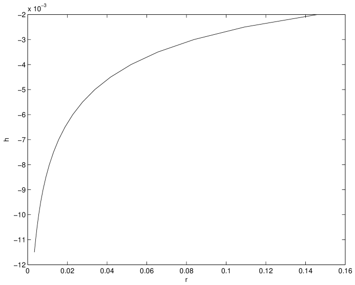
Figure 1: Limit of log of the early exercise boundary at expiry, as a function of the riskless rate. Parameters (ibm1111): $\nu=1.0102;c=0.42;{\lambda_{+}}=4.37;{\lambda_{-}}=-191.20$, $\sigma=0.428$.

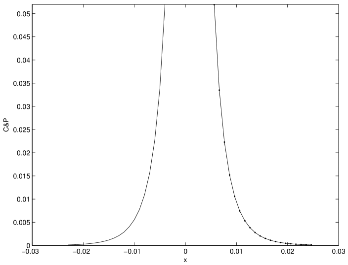
Figure 2: Time decay of the out-of-the-money call and put, at expiry. Parameters (ibm1111): $\nu=1.0102;c=0.42;{\lambda_{+}}=4.37;{\lambda_{-}}=-191.20$, $\sigma=0.428$.

Example 5.1. Only in one case: ibm1111, the process is of order $\nu>1$: the risk-neutral parameters are $\nu=1.0102;c=0.42;{\lambda_{+}}=4.37;{\lambda_{-}}=-191.20$, and $\sigma=0.428$ (in Carr et al., these parameters are denoted $Y,C,G,-M$, and $\eta$). Since $\nu>1$, the non-standard behavior of the early exercise boundary is guaranteed but the gap between the strike price and boundary is small unless the interest rate is very small indeed. It is seen from Figure 1, where we plot the graph of $\bar{h}$ as a function of $r$, that for $r=0.02$, $\bar{h}$ is about $0.006$, and for $r=0.005$, $\bar{h}$ is close to 0.01, so the gap is clearly seen. In Figure 2, we plot the graph of $\theta$ at expiry, for out-of-the-money European call and put (graph of ${\mathcal{C}}(x)$, for small $x<0$ near zero, and put, ${\mathcal{P}}(x)$, for $x>0$). Both are unbounded in a neighborhood of $0$. Since the density of positive jumps decays very fast (the steepness parameter ${\lambda_{-}}=-191.20$ is very large), the time decay of out-of-the-money puts is very small unless the spot price is very close to the strike. The density of positive jumps decays faster than the one of negative jumps ($-{\lambda_{-}}>{\lambda_{+}}$), therefore the $\theta$ for the out-of-the-money call is smaller than the one for out-of-the-money put, for the same distance from the strike.

Example 5.2. For amzn1014, the parameters are $\sigma=0.0684;\nu=0.3072;c=4.60;{\lambda_{+}}=1.78;{\lambda_{-}}=-6.29.$ The fairly large $c$ indicates that the intensity of jumps is large, and relatively small values of ${\lambda_{+}}$ and ${\lambda_{-}}$ imply that there are many large jumps, especially negative ones (recall that ${\lambda_{+}}$ characterizes the rate of decay of the density of negative jumps). Therefore, even not very close to expiry, the owner of an out-of-the-money European option can expect that with a non-negligible probability the option will become in-the-money. Hence, the price of these out-of-the-money options is sizable, especially the one of the put. Figure 3 demonstrates this effect. We plot graphs of ${\mathcal{C}}$ and ${\mathcal{P}}$ in a neighborhood of zero.

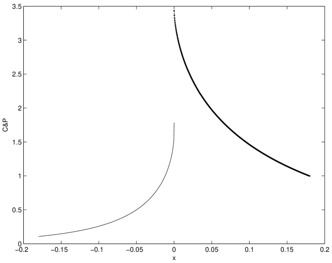
Figure 3: Time decay of out-of-the-money European call and put, at expiry. Parameters (amzn1014): $\nu=0.3072;c=4.60;{\lambda_{+}}=1.78;{\lambda_{-}}=-6.29,\sigma=0.0684.$

Further, ${\mathcal{C}}(-0)=1.7851$, therefore for reasonable $r$, we have $r<{\mathcal{C}}(-0)$, and the behavior of the early exercise boundary is non-standard. Since the intensity of large negative jumps is significant, the value of waiting is very large, and the gap between the strike and optimal exercise boundary is also large. From (4.15) and Figure 3, we can conclude that even at 5% below the strike, the option value of waiting (the difference between the American put price and the pay-off $1-e^{x}$) is of order $0.5\tau$; $\tau=1$ is one year.

In the next two Figures 4 and 5, we plot the graph of ${\mathcal{C}}$ farther from the strike, and the graph of $\bar{h}$ as the function of $r$.

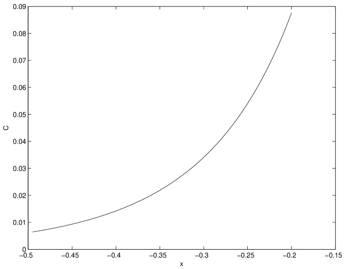
Figure 4: Time decay of out-of-the-money European call, at expiry. Parameters (amzn1014): $\nu=0.3072;c=4.60;{\lambda_{+}}=1.78;{\lambda_{-}}=-6.29,\sigma=0.0684.$

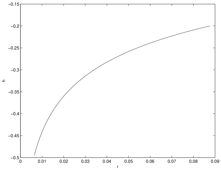
Figure 5: Limit of log of the early exercise boundary, at expiry. Parameters (amzn1014): $\nu=0.3072;c=4.60;{\lambda_{+}}=1.78;{\lambda_{-}}=-6.29,\sigma=0.0684.$

In Figure 6, we plot both the early exercise boundary, at expiry, $H=\exp(\bar{h}(r))$, as a function of $r$, and that of the early exercise boundary far from expiry, $H_{\ast}=\exp(h_{\ast}(r))$ (the early exercise boundary in the infinite time horizon case).

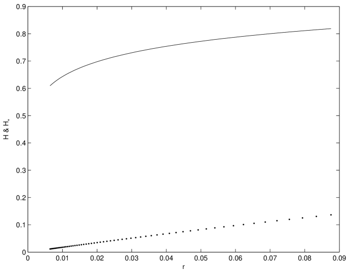
Figure 6: Graphs of the early exercise boundary, at expiry (solid line), and far from expiry (dotted line), as functions of the riskless rate. Parameters (amzn1014): $\nu=0.3072;c=4.60;{\lambda_{+}}=1.78;{\lambda_{-}}=-6.29,\sigma=0.0684.$

Similar results are valid for the other stocks documented in Carr et al. (2002).

7 Conclusion

For several families of Lévy processes used in empirical studies of financial markets, we have proved that the time decay of out-of-the-money European options at expiry is not negligible, and derived explicit formulas. These formulas can be used to make numerical calculations near expiry more accurate – both for European options, and American ones. By using the same formulas, we proved that the optimal exercise boundary for the American put is separated from the strike price by a non-vanishing margin on the interval $[0,T)$, and that as the riskless rate vanishes, the optimal exercise price goes to zero uniformly over the interval $[0,T)$. The last result may be especially interesting since the current levels of interest rates are rather low. Furthermore, we discussed the restrictions on the process under the risk-neutral measure which the non-Gaussian behavior of the early exercise price near expiry imposes, and suggested a natural asymmetric extension of the KoBoL family (a.k.a. CGMY model), which can be used for any type of the behavior of the boundary. We showed that for the risk-neutral parameters obtained for several stocks in Carr et al. (2002), the behavior should be non-standard, and the margin between the strike and the early exercise boundary be quite sizable: more than 10%, up to expiry. The jump premium over the payoff is shown to be sizable as well.

Appendix A Technical proofs

A.1 Proof of Lemma 3.2

First, we consider processes without the Gaussian component, and in the end prove that the results remain the same after an addition of a Gaussian component.

Further, we assume that ${\lambda_{-}}<-1$; the results for the case ${\lambda_{-}}=-1$ obtain by passing to the limit ${\lambda_{-}}\uparrow-1$ in the formulas for the case ${\lambda_{-}}<-1$. For any $\sigma\in({\lambda_{-}},-1)$, the price of the European call option is given by

$${\mathcal{C}}(x,\tau)=(2\pi)^{-1}\int_{-\infty+i\sigma}^{+\infty+i\sigma}\frac{\exp[ix\xi-\tau(r+\psi(\xi))]}{-i\xi(1-i\xi)}d\xi$$ (A.1)

(see e.g. Boyarchenko and Levendorskiǐ (1999, 2002b)). Clearly, the limit ${\mathcal{C}}(x)$ is independent of $r$, therefore we may set $r=0$. The characteristic exponent of a process without the Gaussian component is of the form

$$\psi(\xi)=-i\mu\xi+\phi(\xi),$$

where $\phi(\xi)$ grows as $|\xi|^{\nu}$ in the complex plane with the cuts $(-i\infty,i{\lambda_{-}}]$ and $[i{\lambda_{+}},+i\infty)$, for processes of order $\nu\in(0,2)$. in the complex plane outside two poles $\xi=i\lambda_{\pm}$. For VGP, $\phi(\xi)$ grows as $\ln|z|$, and for exponential jump processes, $\phi(\xi)$ decays as $|\xi|^{-1}$.

Set $x^{\prime}=x+\mu\tau$, and write (A.1) as

$$\tau^{-1}{\mathcal{C}}(x,\tau)=(2\pi)^{-1}\int_{-\infty+i\sigma}^{+\infty+i\sigma}\tau^{-1}\frac{\exp[ix^{\prime}\xi-\tau\phi(\xi)]}{-i\xi(1-i\xi)}d\xi.$$ (A.2)

Let $X_{t}$ be a KoBoL or NTS Lévy process of order $\nu\in(0,1)$. Then we can find $\delta>0$ s.t. $\rho:=(1-\delta)/\nu>1$. Since $\Re\phi(\xi)$ is bounded away from zero on the line $\Im\xi=\sigma$, the integrand in (A.2) admits an upper bound via $C\tau^{-1}(1+|\xi|)^{-2}.$ It follows that the integral over $|\Im\xi|\geq\tau^{-\rho}$ makes a contribution of order

$$2C\tau^{-1}\int_{\tau^{-\rho}}^{+\infty}\eta^{-2}d\eta=2C\tau^{\rho-1}=o(1),\quad{\rm as}\ \tau\to+0.$$

Since $|\phi(\xi)|\leq C(1+|\xi|)^{\nu}$, we have $\tau\phi(\xi)=O(\tau^{\delta})=o(1)$ on the set $\{\xi\ |\ \Im\xi=\sigma,|\Re\xi|\leq\tau^{-\rho}\}$. Hence, we may write (A.2) as

$$\tau^{-1}{\mathcal{C}}(x,\tau) = (2\pi\tau)^{-1}\int_{-\infty+i\sigma}^{+\infty+i\sigma}\frac{e^{ix^{\prime}\xi}(1-\tau\phi(\xi))}{-i\xi(1-i\xi)}d\xi+o(1)$$ (A.4)

$$= (2\pi\tau)^{-1}\int_{-\infty+i\sigma}^{+\infty+i\sigma}\frac{e^{ix^{\prime}\xi}}{-i\xi(1-i\xi)}d\xi$$

$$+(2\pi)^{-1}\int_{-\infty+i\sigma}^{+\infty+i\sigma}\frac{e^{ix^{\prime}\xi}(-\phi(\xi))}{-i\xi(1-i\xi)}d\xi+o(1).$$

The $x<0$ is fixed, therefore for sufficiently small $\tau>0$, $x^{\prime}$ is negative and bounded away from zero, and therefore, $\Re(ix^{\prime}\xi)$ is negative and bounded away from zero, uniformly in $\tau\to+0$ and $\xi$ in the half-plane $\Im\xi\leq\sigma$. This means that we can use the Cauchy theorem and push the line of the integration in (A.4) down: $\sigma\to-\infty$, and obtain that the integral in (A.4) is zero. Hence,

$$\tau^{-1}{\mathcal{C}}(x,\tau)=(2\pi)^{-1}\int_{-\infty+i\sigma}^{+\infty+i\sigma}\frac{e^{ix^{\prime}\xi}(-\phi(\xi))}{-i\xi(1-i\xi)}d\xi+o(1).$$ (A.5)

By using essentially the same argument as in Boyarchenko and Levendorskiǐ (2002b), where a similar integral (5.33) was transformed to the integral over the banks of the cut $(-i\infty,i{\lambda_{-}}]$ in the complex plane, and after the change of variables $\xi=iz-0$ and $\xi=iz+0$ on the left and right banks, respectively, to an integral over $(-\infty,{\lambda_{-}})$ (equation (5.37) in Boyarchenko and Levendorskiǐ (2002b)), we obtain, for $x^{\prime}<0$,

$$\tau^{-1}{\mathcal{C}}(x,\tau)=(2\pi)^{-1}\int_{-\infty}^{\lambda_{-}}\frac{e^{-x^{\prime}z}\Psi(z)}{z(1+z)}dz+o(1).$$ (A.6)

As $\tau\to 0$, $x^{\prime}\to x$, therefore by passing to the limit in (A.6), we obtain (3.10).

Recall that the calculations above were made for a KoBoL or NTS Lévy process of order $\nu\in(0,1)$. If $X_{t}$ is a VGP, then we make essentially the same argument by using any $\rho>0$. If $X_{t}$ is a Hyperbolic Process, NIG, or KoBoL or NTS Lévy process of order $\nu\in(1,2)$, then we start with the integration by part in (A.2), by using

$$e^{ix^{\prime}\xi}d\xi=(ix^{\prime})^{-1}de^{ix^{\prime}\xi}.$$

After that we obtain an absolutely converging integral, and can repeat the constructions above with straightforward changes. In the end, we obtain

$$\tau^{-1}{\mathcal{C}}(x,\tau)=(2\pi x^{\prime})^{-1}\int_{-\infty}^{\lambda_{-}}e^{-x^{\prime}z}\left[\frac{\Psi^{\prime}(z)}{z(1+z)}+\Psi(z)\left(\frac{1}{z(1+z)}\right)^{\prime}\right]dz+o(1).$$

By integrating by part back, and passing to the limit $\tau\to+0$, we obtain (3.10).

To finish the proof of (3.10), it remains to show that the result does not change when we add a Gaussian component. Let $X_{t}$ be any of the processes above, without a Gaussian component, and let $X_{\sigma,t}$ be a Lévy process with the same “drift” term and jump density as $X_{t}$, and with the diffusion coefficient $\sigma^{2}$. Let $p_{\sigma,t}$ be the probability density of $X_{\sigma,t}$, and $p_{G,\sigma,t}$ be the probability density of the Brownian motion with the volatility $\sigma^{2}$. The $p_{G,\sigma,t}$ is the convolution of $p_{t}$ and $p_{G,\sigma,t}$, therefore for $x>0$,

$$\tau^{-1}{\mathcal{C}}(x,\tau) = \int^{+\infty}_{0}\tau^{-1}p_{\sigma,\tau}(y-x)(e^{y}-1)dy$$

$$= \int^{+\infty}_{0}\left(\int_{-\infty}^{+\infty}\tau^{-1}p_{G,\sigma,\tau}(z)p_{\tau}(y-x-z)dz\right)(e^{y}-1)dy$$

$$= \int_{-\infty}^{+\infty}p_{G,\sigma,\tau}(z)\int^{+\infty}_{0}\tau^{-1}p_{\tau}(y-x-z)(e^{y}-1)dydz.$$

Take $\rho\in(1/2,1)$. In the region $|z|\geq\tau^{\rho}$, the Gaussian density is $O(\tau^{N})$, for any $N$, therefore we may replace the outer integral with the integral over $z<\tau^{\rho}$, and add $o(1)$. But then on the support of the integrand, for a fixed $x<0$, $y-x-z$ is bounded away from zero, uniformly in $\tau$. Define ${\mathcal{C}}_{jump}(x)$ as ${\mathcal{C}}(x)$ but assuming that the log-price follows the jump part of the process. Then we can represent the inner integral in the form

$${\mathcal{C}}_{jump}(x+z)+o(1),$$

and therefore,

$$\tau^{-1}{\mathcal{C}}(x,\tau)=\int_{-\infty}^{\tau^{\rho}}p_{G,\sigma,\tau}(z){\mathcal{C}}_{jump}(x+z)dz+o(1).$$

Now, define ${\mathcal{C}}_{jump}(y)$ to be ${\mathcal{C}}_{jump}(x/2)$ for all $y>x/2$. Then for small $\tau$, the integral above does not change but now ${\mathcal{C}}_{jump}$ is a continuous bounded function on ${\bf R}$. By using the super-exponential decay of the Gaussian density, we can restore the $\int_{-\infty}^{+\infty}$, and after that pass to the limit and obtain ${\mathcal{C}}(x)={\mathcal{C}}_{jump}(x)$. This finishes the proof of (3.10).

The proof of (3.11) is similar, only we start with the formula for the European put:

$${\mathcal{P}}(x,\tau)=(2\pi)^{-1}\int_{-\infty+i\sigma}^{+\infty+i\sigma}\frac{\exp[ix\xi-\tau(r+\psi(\xi))]}{-i\xi(1-i\xi)}d\xi,$$

where $\sigma\in(0,{\lambda_{+}})$, and push the contour of the integration up.

A.2 Proof of (3.12)–(3.17), and (3.5)–(3.6) for jump processes with non-zero drift

If $X_{t}$ is a VGP, KoBoL or NTS Lévy process, then it suffices to calculate $\Psi(z)$ and substitute the results in (3.10) and (3.11).

1. Let $X_{t}$ be a VGP. We have

$$\Psi(z)=ci[\ln({\lambda_{+}}-z+i0)+\ln(-{\lambda_{-}}+z-i0)-\ln({\lambda_{+}}-z-i0)-\ln(-{\lambda_{-}}+z+i0)].$$

If $z>{\lambda_{+}}$, then the terms with ${\lambda_{-}}$ cancel out, and

$$\ln({\lambda_{+}}-z\pm i0)=\ln(z-{\lambda_{+}})\pm i\pi.$$

Hence, $\Psi(z)=-c2\pi$. If $z<{\lambda_{-}}$, then the terms with ${\lambda_{+}}$ cancel out, and

$$\ln(-{\lambda_{-}}+z\pm i0)=\ln(z+{\lambda_{-}})\pm i\pi.$$

Thus, $\Psi(z)=c2\pi$.

2. Let $X_{t}$ be a KoBoL process. In the case $z>{\lambda_{+}}$,

$$\Psi(z) = ic\Gamma(-\nu)[-({\lambda_{+}}-z+i0)^{\nu}-(-{\lambda_{-}}+z-i0)^{\nu}$$

$$\hskip 45.52458pt+({\lambda_{+}}-z-i0)^{\nu}+(-{\lambda_{-}}+z+i0)^{\nu}]$$

$$= ic\Gamma(-\nu)[({\lambda_{+}}-z-i0)^{\nu}-({\lambda_{+}}-z+i0)^{\nu}]$$

$$= ic\Gamma(-\nu)(z-{\lambda_{+}})^{\nu}i(e^{-i\pi\nu}-e^{i\pi\nu})$$

$$= 2c\Gamma(-\nu)\sin(\pi\nu)(z-{\lambda_{+}})^{\nu}.$$

Similarly, in the case $z<{\lambda_{-}}$,

$$\Psi(z)=-2c\Gamma(-\nu)\sin(\pi\nu)(-z+{\lambda_{-}})^{\nu}.$$

3. Let $X_{t}$ be an NTS Lévy process. If $z>{\lambda_{+}}=\alpha+\beta$, then

$$\Psi(z) = i\delta[(\alpha^{2}-(\beta+i(iz+0)^{2})^{\nu/2}-(\alpha^{2}-(\beta+i(iz-0)^{2})^{\nu/2}]$$

$$= i\delta[(\alpha^{2}-(\beta-z+i0)^{2})^{\nu/2}-(\alpha^{2}-(\beta-z-i0)^{2})^{\nu/2}]$$

$$= i\delta(\alpha-\beta+z)^{\nu/2}[(\alpha+\beta-z+i0)^{\nu/2}-(\alpha+\beta-z-i0)^{\nu/2}]$$

$$= i\delta(\alpha-\beta+z)^{\nu/2}(z-\alpha-\beta)^{\nu/2}(e^{i\pi\nu/2}-e^{-i\pi\nu/2})$$

$$= -2\sin\frac{\pi\nu}{2}((z-\beta)^{2}-\alpha^{2})^{\nu/2}.$$

If $z<{\lambda_{-}}=-\alpha+\beta$, then similarly, we obtain the same expression but without the minus sign.

Finally, if $X_{t}$ is an exponential jump-diffusion process, then the same proof as in Lemma 3.2 shows that for the call, it suffices to consider the pure jump process, and that in this case, (A.5) holds. Since

$$\phi(\xi)=\frac{ic_{+}\xi}{{\lambda_{+}}+i\xi}+\frac{ic_{-}\xi}{{\lambda_{-}}+i\xi},$$

the integrand in (A.5) has the only pole $\xi=i{\lambda_{-}}$ in the plane $\Im\xi\leq\sigma$. We push down the line of integration, and on crossing the pole, apply the residue theorem. The result is

$$\tau^{-1}{\mathcal{C}}(x,\tau) = -(2\pi i)^{-1}\int_{-\infty+i\sigma}^{+\infty+i\sigma}\frac{e^{ix^{\prime}\xi}ic_{-}\xi}{-i\xi(1-i\xi)(\xi-i{\lambda_{-}})}d\xi+o(1)$$

$$= \left.\frac{e^{ix^{\prime}\xi}c_{-}}{-1+i\xi}\right|_{i\xi=-{\lambda_{-}}}+o(1),$$

and by passing to the limit, we obtain (3.6). (3.5) is proved similarly.

References

1. Aıt-Sahalia, Y.: Disentangling diffusion from jumps. Forthcoming in Journal of Financial Economics (2003)

2. Aıt-Sahalia, Y.: Telling from discrete data whether the underlying continuous-time model is a diffusion. Journal of Finance 57, 2075-2112 (2002)

3. Barles, G., Burdeau, J., Romano, M., and Samsoen, N.: Critical stock price near expiration. Mathematical Finance. 5, 77-95 (1995)

4. Barndorff-Nielsen, O. E.: Exponentially decreasing distributions for the logarithm of particle size. Proceedings of the Royal Society. London. Ser. A. 353, 401–419 (1977)

5. Barndorff-Nielsen, O. E.: Processes of Normal Inverse Gaussian Type. Finance and Stochastics. 2, 41–68 (1998)

6. Barndorff-Nielsen, O. E., and Jiang, W.: An initial analysis of some German stock price series. Working Paper Series 15, CAF Univ. of Aarhus/Aarhus School of Business, October 1998.

7. Barndorff-Nielsen, O. E., and Levendorskiǐ, S.: Feller Processes of Normal Inverse Gaussian type. Quantitative Finance. 1, 318–331 (2001)

8. Barndorff-Nielsen, O. E., and Shephard, N.: Normal modified stable processes. Forthcoming in Theory of Probability and Mathematical Statistics

9. Bouchaud, J-P., and Potters, M.: Theory of Financial Risk. Paris: Aléa-Saclay, Eurolles 1997

10. Boyarchenko, S.I., Levendorskiǐ, S.Z.: Generalizations of the Black-Scholes equation for truncated Lévy processes. Working Paper. University of Pennsylvania, Philadelphia 1999

11. Boyarchenko, S.I., Levendorskiǐ, S.Z.: Option Pricing for Truncated Lévy Processes. International Journal of Theoretical and Applied Finance. 3:3, 549–552 (2000)

12. Boyarchenko, S.I., Levendorskiǐ, S.Z.: Perpetual American Options under Lévy Processes. SIAM Journal of Control and Optimization. 40:6, 1663–1696 (2002a)

13. Boyarchenko, S.I., Levendorskiǐ, S.Z.: Non-Gaussian Merton-Black-Scholes theory. Singapore: World Scientific 2002b

14. Boyarchenko, S.I., Levendorskiǐ, S.Z.: Barrier options and touch-and-out options under regular Lévy processes of exponential type. Annals of Applied Probability. 12:4, 1261–1298 (2002c)

15. Carr, P.: Randomization and the American put. Review of Financial Studies. 11, 597-626 (1998)

16. Carr, P., and Faguet, D.: Fast accurate valuation of American options. Working paper. Cornell University, Ithaca 1994

17. Carr, P., Geman, H., Madan, D.B., and Yor, M.: The fine structure of asset returns: an empirical investigation. Journal of Business. 75, 305-332 (2002)

18. Carr, P., and Hirsa, A.: Why be backward?. Risk, January 2003, 26, 103–107 (2003)

19. Carr, P., and Wu, L.: What type of process underlies options? A simple robust test. Journal of Finance. 57, 2581–2610 (2003)

20. Clément, E., Lamberton, D., and Protter, P.: An analysis of a least squares regression method for American option pricing. Finance and Stochastics. 6, 449-471 (2002)

21. Cont, R., Potters, M., and Bouchaud, J.-P.: Scaling in stock market data: stable laws and beyond”, in Dubrulle, B., F. Graner, and D. Sornette (eds.). Scale Invariance and beyond (Proceedings of the CNRS Workshop on Scale Invariance, Les Houches, March 1997). Berlin: Springer 1997

22. Eberlein, E., and Keller, U. Hyperbolic distributions in finance. Bernoulli. 1, 281–299 (1995)

23. Eberlein, E., Keller, U., and Prause, K.: New insights into smile, mispricing and value at risk: The hyperbolic model. Journal of Business. 71, 371–406 (1998)

24. Eberlein, E., and Raible, S.: Term structure models driven by general Lévy processes. Mathematical Finance. 9, 31–53 (1999)

25. Hirsa, A., and Madan, D.B.: Pricing American options under Variance Gamma. Journal of Computational Finance, forthcoming (2003)

26. Karatzas, I., and Shreve, S.E.: Methods of Mathematical Finance. Springer-Verlag: Berlin Heidelberg New York (1998)

27. Koponen, I.: Analytic approach to the problem of convergence of truncated Lévy flights towards the Gaussian stochastic process. Physics Review E. 52, 1197–1199 1995

28. Lamberton, D.: Critical price for an American option near maturity. In Bolthausen, E. , M. Dozzi, F. Russo (eds.) Seminar on Stochastic Analysis, Random Fields and Applications. Boston Basel Berlin: Birkhaüser 1995

29. Levendorskiǐ, S. Z.: Pricing of American put under Lévy processes. To appear in International Journal of Theoretical and Applied Finance

30. Longstaff, F.A., and Schwartz, E.S.: Valuing American options by simulation: a simple least-squares approach. Review of Financial Studies. 14, 113-148 (2001)

31. Madan, D. B., Carr, P., and Chang, E. C.: The variance Gamma process and option pricing. European Finance Review. 2, 79–105 (1998)

32. Matacz, A.: Financial modeling and option theory with the Truncated Levy Process. International Journal of Theoretical and Applied Finance. 3, 143-160 (2000)

33. Musiela, M., and Rutkowski, M.: Martingale methods in financial modelling. Berlin Heidelberg New York: Springer-Verlag 1997

34. Sato, K.: Lévy processes and infinitely divisible distributions. Cambridge: Cambridge University Press 1999