Exponents of the localization length in the 2D Anderson model with off-diagonal disorder

Abstract.

We study Anderson localization in two-dimensional systems with purely off-diagonal disorder. Localization lengths are computed by the transfer-matrix method and their finite-size and scaling properties are investigated. We find various numerically challenging differences to the usual problems with diagonal disorder. In particular, the divergence of the localization lengths close to the band centre is investigated in detail for bipartite and non-bipartite lattices as well as different distributions of the off-diagonal disorder. Divergence exponents for the localization lengths are constructed that appear to describe the data well down to at least $10^{-5}$. We find only little evidence for a crossover energy scale below which the power law has been argued to fail.

1. Introduction

The disorder-induced metal-insulator transition and the concept of Anderson localization [1, 2, 3, 4, 5] have been the subject of an intense research for more than forty years. The highly successful scaling approach for non-interacting electrons was proposed by Abrahams et al. [6] in 1979, predicting that for generic situations in 1D and 2D all states remain localized, thus there is no disorder-driven transition [7, 8, 9]. However, it was suggested [10, 11, 12] that an Anderson model with purely off-diagonal disorder may be an exception, as non-localized states were found at the band center [13, 14, 15, 16, 17]. Recent numerical investigations [18, 19, 20, 21, 22, 23] have revealed unusual localization properties of these states. It was found that the localization length diverges at the energy $E=0$ [18, 19], scaling properties of this divergence suggest that the states at the band center are critical [19, 23], thus there are no truly extended states in 2D in agreement with the scaling arguments.

Of special interest is the model of off-diagonal disorder on the bipartite lattice with even number of sites, which exhibits special symmetry properties at the band center — the energy spectrum is symmetric around $E=0$. It has been shown that in this case, related to the chiral universality class [24, 25], states at the band center are non-localized in any dimension [12, 26, 27]. This has been recently demonstrated in 2D and 3D using a renormalization group (RG) approach [28]. In a recent paper [29], we studied 2D bipartite systems with various types of off-diagonal disorder by means of the transfer-matrix method (TMM) and investigated the divergence of the localization lengths close to the band center. In Ref. [28] it has been suggested that this divergence may be described by

$$\xi(E)\propto\left|\frac{E_{0}}{E}\right|^{\nu},\quad|E|>E^{*},\quad\hfil\mbox{and}\hfil\quad\xi(E)\propto\exp\sqrt{\frac{\ln E_{0}/E}{A}},\quad|E|<E^{*}$$ (1)

with a certain, unspecified crossover energy $E^{*}$ distuinguishing between the power law and the more complicated form. In [29] we showed that a power-law behavior fits the data down to energy $E=2\times 10^{-5}$ and the corresponding divergence exponents $\nu$ have rather low values $\sim 0.3$ that seem to depend non-universally on the type and strength of the disorder. In this paper we extend these calculations to energies even closer to the band center at $E=0$. In addition to the square 2D lattices we examine also honeycomb lattices where the Van Hove singularity at $E=0$ does not interfere with the divergence due to the chiral symmetry.

2. The Hamiltonian, off-diagonal disorder distributions and the transfer-matrix method

The Anderson Hamiltonian for a single electron on a 2D lattice is

$$H=\sum_{i\neq j}^{N}t_{ij}\left|i\right\rangle\left\langle j\right|+\sum_{i}^{N}\epsilon_{i}\left|i\right\rangle\left\langle i\right|$$ (2)

where $\left|i\right\rangle$ denotes the electron wave function at site $i$. For purely off-diagonal disorder, we set the onsite energies $\epsilon_{i}$ to $0$. The off-diagonal disorder is introduced by random hopping elements $t_{ij}$ between nearest neighbor sites. In a square lattice all four hopping elements to the four nearest neighbor are chosen according to the random distribution. The honeycomb lattice [30] is topologically equivalent to the brick-layer structure [31] — the corresponding hopping element of the underlying square lattice is equal $0$.

On both lattices we study three different distributions of off-diagonal elements $t_{ij}$,

$$P\left(t_{ij}\right) =\left\{\begin{array}[]{ll}1/w&\textrm{if $\left|t_{ij}-c\right|\leq w/2$,}\\ 0&\textrm{otherwise,}\end{array}\right. \mbox{a box distribution \cite[cite]{[\@@bibref{}{EilRS98a}{}{}]}},$$ (5)

$$P\left(t_{ij}\right) =\frac{1}{\sqrt{2\pi\sigma^{2}}}\exp\left[-\frac{\left(t_{ij}-c\right)^{2}}{2\sigma^{2}}\right], \mbox{a Gaussian distribution},$$ (6)

$$P\left(\ln t_{ij}/t_{0}\right) =\left\{\begin{array}[]{ll}1/w&\textrm{if $\left|\ln t_{ij}/t_{0}\right|\leq w/2$,}\\ 0&\textrm{otherwise.}\end{array}\right. \mbox{a box distribution for $\ln t_{ij}$ \cite[cite]{[\@@bibref{}{SouWGE82}{}{}]}}.$$ (9)

The logarithmic $t$ ($\ln t$) distribution is believed to be more suitable to model actual physical systems [17] and the parameter $w$ is a good measure for the off-diagonal disorder strength. We will show however, that although it directly avoids problems with zero $t$ elements present in the case of box and Gaussian distributions [18], for larger $w$ values it is likely to suffer similar numerical problems due to a large number of small elements close to $\exp(-w)$.

The TMM [32, 33] is widely used to study the localization properties of states in disordered systems. To calculate the decay lengths of wave functions on quasi-1D strips of width $M$ and length $K\gg M$ the Schrödinger equation for the Hamiltonian (2) is written in the TMM form:

$$\left(\begin{array}[]{c}\psi_{n+1}\\ \psi_{n}\end{array}\right)=\left(\begin{array}[]{cc}[t^{||}_{n+1}]^{-1}(E-\epsilon_{n}-H_{\perp})&-[t^{||}_{n+1}]^{-1}t^{||}_{n}\\ 1&0\end{array}\right)\left(\begin{array}[]{c}\psi_{n}\\ \psi_{n-1}\end{array}\right)=T_{n}\left(\begin{array}[]{c}\psi_{n}\\ \psi_{n-1}\end{array}\right),$$ (10)

where $\psi_{n}=(\psi_{n,1},\psi_{n,2},\ldots,\psi_{n,M})^{T}$ denotes the wave function at all sites of the $n$th slice, $\epsilon_{n}={\rm diag}(\epsilon_{n,1},\ldots,\epsilon_{n,M})$, $H_{\perp}$ is the hopping Hamiltonian within slice $n$ and $t^{||}_{n}=$ ${\rm diag}(t^{||}_{n,1}$, $t^{||}_{n,2}$, $\ldots$, $t^{||}_{n,M})$ is the diagonal matrix of hopping elements connecting slice $n-1$ with slice $n$. For rectangular and Gaussian distributions of hopping elements we set the width $w$ and the standard deviation $\sigma$ of the distribution to $1$ and center it at the $c=0$. In the case of the $\ln t$ distribution we chose $t_{0}=1$ which sets the energy scale and perform calculations for two values $w=2$ and $6$ of the distribution width.

In the case of the honeycomb lattice half of the connections to the nearest neighbors perpendicular to the TMM direction are missing, thus the lattice topology is reflected in the $H_{\perp}$ part of the Hamiltonian. The largest localization length $\lambda(E,M)=1/\gamma_{\rm min}$ at energy $E$ and strip width $M$ is determined by the smallest Lyapunov exponent $\gamma_{\rm min}>0$ obtained as the eigenvalue closest to one of the product of the transfer matrices $\tau_{K}=T_{K}T_{K-1}\ldots T_{2}T_{1}$ when $K\rightarrow\infty$ [34].

After calculating localization lengths $\lambda(M)$ for increasing widths of the strips $M$ we scaled the reduced localization lengths $\lambda(M)/M$ onto a single scaling curve

$$\lambda(M)/M=f(\xi/M).$$ (11)

The scaling function and the values of the scaling parameter $\xi$ were determined by the finite-size scaling (FSS) procedure as in Ref. [33]. As we will explain below, the recent FSS approach as outlined in Refs. [35, 36] in not applicable here since the functional form of the divergence of $\xi(E)$ for $E\rightarrow 0$ is not yet clear.

3. Singularities in the density of states

The square lattice without disorder exhibits a van-Hove singularity in the density of states (DOS) at the band center as shown in Fig. 3. Its properties could mask the Dyson singularity due to the off-diagonal disorder. Thus we also investigate a honeycomb lattice where the van-Hove singularity is absent at $E=0$. In fact the DOS for the ordered system on honeycomb lattices exhibit a dip at $E=0$ [31]. With increasing off-diagonal disorder the DOS at this energy increases and for large disorders it becomes as large as for square lattices. These features are readily visible in Fig. 3. [htb]

Density of states for purely off-diagonal disorder with a $\ln t$ distribution on a square (left) and a honeycomb (right) lattice. The data has been obtained by exact diagonalization of the model (2) for $200\times 200$ sites for one realization of the disorder. The dashed lines correspond to the ordered lattices. In all cases, the energy has been rescaled by the band width and the DOS has not been normalized to integrate to unity. It is worth noting, that for large $w$ values the peak at the band center for the $\ln t$ distribution is much higher than in case of rectangular or Gaussian distribution.

4. Localization properties of bipartite lattices

The TMM calculations are performed for strip widths up to $M=220$ in the energy interval $1\times 10^{-8}\leq E\leq 0.1$, the actual values depend on the disorder parameters. The accuracy of the localization lengths is $1\%$ in all cases.

4.1. Finite-size effects and scaling close to the band center

In Fig. 4.1, we show the behavior of the localization lengths for various strip widths as a function of energy. The $\lambda_{M}/M$ data for small system sizes shows a pronounced bending-down effect close to $E=0$ which is most prominent for even strip widths [22]. For odd strip widths $\lambda_{M}/M$ monotonically increases (in the examined energy range) as the energy approaches $0$, although for the smallest width it is almost constant close to the band center (4.1, right panel). [thb]

Reduced localization lengths $\lambda_{M}/M$ on a square lattice as function of energy $E$ at disorder $w=6$. Left: even system widths ranging from $M=10$ ($\circ$), $20$ ($\Box$), to $100$ ($*$); Right: odd widths from $M=15$ ($\circ$), $25$ ($\Box$), to $105$ ($*$).

Clearly, such a behavior at small $M$ can not be captured easily in an FSS procedure. Therefore we only use system widths large enough such that the bending for small energies is irrelevant. Of course this increases the computational effort necessary. Furthermore, the accessible strip widths will depend on the value of the disorder parameter and energy, smaller values requiring much more time. In Table 1 we show the list of values used.

Table 1. Estimated values of the exponents of the localization lengths defined in (1) for various disorder strengths and distributions. The error bars only represent the standard deviations from a power-law fit of (1) to the $\lambda(E,w)$ data and should be increased up to one order of magnitude for a reliable representation of the actual errors.

	square lattice		honeycomb lattice
disorder parameters	sizes used in FSS	$\nu$	sizes used in FSS	$\nu$
box, $c=0$	$150-220$	$0.317\pm 0.007$	$110-170$	$0.290\pm 0.004$
Gaussian, $c=0$	$110-160$	$0.303\pm 0.006$	$120-170$	$0.273\pm 0.005$
$\ln t$, $w=2$	$110-190$	$0.357\pm 0.009$	$100-170$	$0.604\pm 0.015$
$\ln t$, $w=6$	$120-170$	$0.232\pm 0.007$	$120-170$	$0.238\pm 0.007$

Next, an FSS procedure [33] unbiased by any preset fitting function is applied to the data and the infinite-size localization length $\xi$ is extracted. Fig. 1 shows the resulting scaling plots. We emphasize that this FSS procedure does not require any apriori knowledge of which function in (1) is correct and does not make any assumptions in the general form of the scaling function $f$. [htb]

FSS plots of $\lambda_{M}(E,w)/M$ for square (left) and honeycomb (right) lattices. Note that data for different disorder distributions can be scaled simultaneously, except for the numerically most challenging $\ln t$ data at $w=2$ as shown in the right panel. We also calculate error estimates for $\xi$ taking into account the accuracy of the raw localization lengths $\lambda$. Namely, we repeat the FSS procedure several hundred times changing randomly the input localization lengths $\lambda$ within its $1\%$ accuracy (of a Gaussian distribution). Then we calculate the standard deviation of the obtained values of the scaling parameter. The errors — as shown in the figures below — typically increase close to $E=0$ and are larger when larger strip widths are used in FSS.

4.2. Divergence of the localization lengths and further finite-size effects

To investigate the divergence of the infinite-size localization lengths at the band center we plot the scaling parameter $\xi$ in a doubly logarithmic plot [37]. The deviation of the divergence from the power-law behavior should be then easily seen. In most cases we observe that at energies close to $E=0$ the divergence is slower than described by a power-law. Two examples are shown in Fig. 4.2. [htb]

Scaling parameter $\xi$ as function of energy for a square lattice and Gaussian disorder distribution (left) and a honeycomb lattice with $\ln t$ disorder distribution at $w=6$ (right). The small, filled symbols denote results for system widths $M=50$–$100$ and have been shifted downwards by $\log_{10}0.25$ (left panel) and $\log_{10}0.2$ (right panel) for clarity. The large, open symbols indicate results for $M=110$–$160$ (Gaussian distribution) or $M=100$–$150$ ($\ln t$ distribution). The left panel presents a log-log plot of the energy dependence of the scaling parameter $\xi$ for a Gaussian $t$ distribution with $c=0$ on a square lattice. The curve obtained for smaller strip widths $M=50-100$ exhibits clear deviations from the straight line for smaller energies. However, for larger widths ($M=110-160$) this deviation gets smaller and the dependence is power-law in a wider energy range. Generally, in the energy range where the $\lambda_{M}$ for small widths $M$ decreases close to $E=0$ or diverges slower than for larger $M$, one can observe that the values of the scaling parameter $\xi$ resulting from the FSS are too small compared to the values obtained for larger systems, which is manifested as a deviation from the power-law behavior of the localization lengths.

Therefore, the deviations from the power-law behavior as in Fig. 4.2 appear to be finite-size effects that remain even after FSS. We performed such a check for all disorders and disorder distributions. It turns out that in almost all cases when the scaling parameter exhibits a deviation from the power-law, this deviation is smaller for larger system sizes, thus may be attributed to finite-size. The only exception is the $\ln t$ distribution for $w=6$. An example for a hexagonal lattice is shown in the right panel of Fig. 4.2. In this case the results appear not to change with the system size, thus the bending down of the line close to the band center may reflect the change in the behavior of the localization length, i.e., a crossover from power-law to the exponential form as in Eq. (1).

4.3. Numerical problems for off-diagonal disorder with small $t$ and $\ln t$ distribution

From the TMM equation (10) it follows that the division by hopping elements $t^{||}_{n+1}$ is necessary to calculate the wave function in the next step of TMM. This may be a source of potential numerical problems if the hopping elements are very close to zero. In the case of rectangular and Gaussian distribution we therefore applied a cutoff for small $|t^{||}_{n+1}|$ values and checked that the results do not depend on the cut-off. Furthermore, even for hopping amplitudes larger than the cut-off, the ratio $[t^{||}_{n+1}]^{-1}t^{||}_{n}$ in Eq. (10) may become large and lead to a large value of the corresponding component of the wave function. In the next steps this large value will grow even further which might lead to the loss of numerical accuracy due to round-off errors. The growth of the wave vector component is normally suppressed by the repeated reorthonormalization of the wave functions. In our calculations we performed the reorthonormalization after a fixed number of 10 TMM steps. We checked that in the case of rectangular and Gaussian disorder distribution this is sufficient to guarantee numerical stability. Note that an automatic reorthogonalization scheme as is customarily used for diagonal disorder does not work so well in the present case of off-diagonal disorder [36].

One might expect that similar problems do not appear in the case of the $\ln t$ distribution as the elements are never zero by definition. However, in the $\ln t$ distribution the most probable hopping elements are small elements $\gtrsim\exp(-w/2)$. Thus there are many large $t$-ratios $\sim\exp(w/2)$ and wave function components. This has a striking effect on the stability of the calculation as shown, e.g., in Fig. 4.3. [htb]

Reduced localization lengths $\lambda_{M}/M$ for square lattice and $\ln t$ distribution. In the left panel, reorthonormalization of the wave functions has been performed after every 10th TMM step. In the right panel, reorthonormalization is being done after each TMM step. When the number of TMM steps between renormalizations is kept at $10$, the localization lengths seem to indicate localized behavior for increasing $w$ values. However, renormalizing after each TMM step, we see that there is no localization, rather, the states remain critical. Let us emphasize that this effect appears for larger disorder where naively one would expect numerical stability to become better (as for diagonal disorder). Generally, all runs with $w>6$ need to be done with renormalization after each TMM step. It is also worth noting that, as the wave function may grow in one TMM step up to $\exp(w)$, for sufficiently large $w$ numerical problems will arise even if the wave functions are normalized after each TMM step.

In the present manuscript, we therefore calculate our localization lengths for $w=6$ disorders using reorthonormalization after each $5$th TMM step.

4.4. Estimates of the divergence exponents

In Figs. 4.4 and 1 we show the dependence of the scaling parameter $\xi$ versus the energy in the double-logarithmic plot for rectangular, Gaussian and logarithmic $t$ distributions, respectively. [htb]

Variation of the infinite-size localization length $\xi$ with $E$ for rectangular (left) and Gaussian (right) disorder distribution. Squares denote data for a square lattice, diamonds denote a honeycomb lattice. Only the points marked by large symbols were used to fit the straight lines.

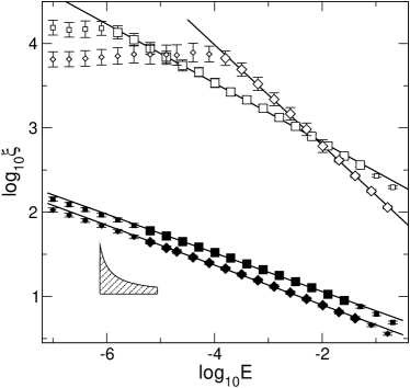
Figure 1. Variation of the infinite-size localization length $\xi$ with $E$ for $\ln t$ disorder distribution with $w=2$ (open symbols) and $w=6$ (filled symbols). Squares denote data for a square lattice, diamonds denote a honeycomb lattice. Only the points marked by large symbols were used to fit the straight lines.

The corresponding exponents are collected in Table 1. They are all in the range of $0.2-0.6$. The values depend on the disorder distribution and parameters, generally the exponents are larger for weaker disorders when the localization lengths are larger. The differences between square and honeycomb lattices appear smaller than the error for most distributions except for the $\ln t$ distribution with $w=2$. In that case the exponent is almost $2$ times larger on the honeycomb lattice. Note that this is precisely the case when the DOS do not exhibit a peak at the band center. Thus the large change in the exponent may be related to the low density of states in the case of the hexagonal lattice. Of course, this also makes the calculation of the localization lengths more time consuming therefore for this system we were able to obtain the results for relatively large energies only.

We emphasize that the exponents do not fullfill the Chayes criterion $\nu\geq 2/d$ [38] with $d$ the lattice dimensionality. However, this is also not to be expected since this is not a true phase transition and for small energies, we expect the crossover as indicated in Eq. (1).

5. The non-bipartite triangular lattice

As shown in Sec. 4, the localization lengths $\lambda_{M}$ for even and odd system sizes are very similar in the limit of large system widths. Apriori this not obvious since the odd-sized systems are not strictly bipartite due to the periodic boundary conditions. In [28] it was shown that the state at the band center is expected to be critical only for bipartite lattices. The breakdown of bipartitness leads to complete localization. In our case, however, the non-bipartitness is only at the boundaries, therefore we find that it is negligible for large enough widths.

Let us now turn to an example of a strictly non-bipartite lattice with off-diagonal disorder such as the triangular lattice shown in Fig. 2.

Figure 2. The two-dimensional triangular lattice. The arrow shows the direction in which the TMM proceeds. The dots indicate lattice site and the solid lines show the connectivity of the lattice. The labelling of each sites in odd and even $n$ slices is indicated.

In the triangular lattice each node is connected to the next and previous slice by two connections instead of one [30]. The TMM equations for this system are similar to Eq. (10) with the exception that the matrices $t^{||}_{n}$ are no longer diagonal. Hence our TMM procedure is essentially the same as for the triangular lattice with diagonal disorder [30], except that the connectivity matrices $t^{||}_{n}$ will now be different for each slice. As before for each TMM step the inversion of the $M\times M$ connectivity matrix $t^{||}_{n}$ must be computed — in practice we solve the equivalent set of linear equations — which significantly increases the computational effort.

We performe the TMM calculations at the energy $E\rightarrow 0$ for system sizes $M=10,20,\ldots,110$ and the centers of the rectangular disorder distribution of hopping elements $c=0,0.1,\ldots,0.5$. The states at the band center are localized for all $c$ values in agreement with [28]. The FSS plot for the data is shown in Fig. 2, where the localized behavior of the states is clearly visible. [htb]

Left: Scaling plot for the triangular lattice with box disorder at E=$0$, $c=0,0.1,\ldots,0.5$ and system sizes $M=10,20,\ldots,100$. Right: dependence of the scaling parameter $\xi$ on the box distribution center $c$. The values of the scaling parameters are shown in the inset; it may be noted that the strongest localization (strongest disorder) appears for $c=0.2$ which is a typical behavior for the chosen rectangular disorder distribution [18].

6. Conclusions

We calculated the localization lengths for different disorder distributions on square and honeycomb lattices. We determined the energy ranges in which the divergence of the localization lengths at the band center is described by a power-law. We also computed the divergence exponents which fall in the range $0.2-0.6$ and seem to depend on the disorder parameters and in some cases on the lattice topology.

For smaller energies we observe deviations from the power-law. However, for most systems these deviations become smaller for larger system widths $M$ and it appears that they are due to finite-size effects that are retained even after FSS. The exception is the $\ln t$ distribution with $w=6$, where below an energy $E\approx 10^{-5}$ we observe a size-independent deviation from the power-law. This may be an indication of the crossover to the non-power-law behavior such as predicted in Ref. [28] or to a power-law with a different exponent. However, there is also a possibility that this may be an still an effect of as of yet unknown further numerical problems which we already encountered for strong $\ln t$ disorder.

It is a pleasure to thank George Rowlands for stimulating discussions.

This article is dedicated to Michael Schreiber on the occasion of his 50th birthday. We are grateful to him for much stimulating material and encouraging structure over the last decade.

References

- [1] P. W. Anderson, Phys. Rev. 109, 1492 (1958).
- [2] E. N. Economou and M. H. Cohen, Phys. Rev. Lett. 25, 1445 (1970).
- [3] E. N. Economou and M. H. Cohen, Phys. Rev. B 5, 2931 (1972).
- [4] E. N. Economou, Journale de Physique C 3, 145 (1972).
- [5] D. C. Licciardello and E. N. Economou, Solid State Commun. 15, 969 (1974).
- [6] E. Abrahams, P. W. Anderson, D. C. Licciardello, and T. V. Ramakrishnan, Phys. Rev. Lett. 42, 673 (1979).
- [7] P. A. Lee and T. V. Ramakrishnan, Rev. Mod. Phys. 57, 287 (1985).
- [8] B. Kramer and A. MacKinnon, Rep. Prog. Phys. 56, 1469 (1993).
- [9] D. Belitz and T. R. Kirkpatrick, Rev. Mod. Phys. 66, 261 (1994).
- [10] E. N. Economou and P. D. Antoniou, Solid State Commun. 21, 285 (1977).
- [11] P. D. Antoniou and E. N. Economou, Phys. Rev. B 16, 3768 (1977).
- [12] F. Wegner, Z. Phys. B 35, 207 (1979).
- [13] T. Odagaki, Solid State Commun. 33, 861 (1980).
- [14] C. M. Soukoulis and E. N. Economou, Phys. Rev. B 24, 5698 (1981).
- [15] A. Fertis, A. Andriotis, and E. N. Economou, Phys. Rev. B 24, 5806 (1981).
- [16] A. Puri and T. Odagaki, Phys. Rev. B 24, 5541 (1981).
- [17] C. M. Soukoulis, I. Webman, G. S. Grest, and E. N. Economou, Phys. Rev. B 26, 1838 (1982).
- [18] A. Eilmes, R. A. Römer, and M. Schreiber, Eur. Phys. J. B 1, 29 (1998).
- [19] A. Eilmes, R. A. Römer, and M. Schreiber, phys. stat. sol. (b) 205, 229 (1998).
- [20] P. Cain, Master’s thesis, Technische Universität Chemnitz, 1998.
- [21] P. Cain, R. A. Römer, and M. Schreiber, Ann. Phys. (Leipzig) 8, SI33 (1999), ArXiv: cond-mat/9908255.
- [22] P. Biswas, P. Cain, R. A. Römer, and M. Schreiber, phys. stat. sol. (b) 218, 205 (2000), ArXiv: cond-mat/0001315.
- [23] S. Xiong and S. N. Evangelou, Phys. Rev. B 64, 113107 (2001).
- [24] M. Bocquet and J. T. Chalker, Phys. Rev. B 67, 054204 (2003).
- [25] C. Mudry, S. Ryu, and A. Furusaki, Phys. Rev. B 67, 064202 (2003), ArXiv: cond-mat/9207723.
- [26] R. Gade and F. Wegner, Nucl. Phys. B 360, 213 (1991).
- [27] R. Gade, Nucl. Phys. B 398, 499 (1993).
- [28] M. Fabrizio and C. Castellani, Nucl. Phys. B 583, 542 (2000), ArXiv: cond-mat/0002328.
- [29] A. Eilmes, R. A. Römer, and M. Schreiber, Physica B 296, 26 (2001).
- [30] M. Schreiber and M. Ottomeier, J. Phys.: Condens. Matter 4, 1959 (1992).
- [31] U. Grimm, R. A. Römer, and G. Schliecker, Ann. Phys. (Leipzig) 7, 389 (1998).
- [32] A. MacKinnon and B. Kramer, Phys. Rev. Lett. 47, 1546 (1981).
- [33] A. MacKinnon and B. Kramer, Z. Phys. B 53, 1 (1983).
- [34] V. I. Oseledec, Trans. Moscow Math. Soc. 19, 197 (1968).
- [35] K. Slevin and T. Ohtsuki, Phys. Rev. Lett. 82, 382 (1999), ArXiv: cond-mat/9812065.
- [36] F. Milde, R. A. Römer, M. Schreiber, and V. Uski, Eur. Phys. J. B 15, 685 (2000), ArXiv: cond-mat/9911029.
- [37] The FSS procedure of Ref. [33] estimates the infinite-size localization lengths from the scaling parameter by extending the calculation to the strongly localized regime where . Here we are not in this regime and thus our are only proportional to the true infinite-size localizaton lengths. However, this is irrelevant when comparing with Eqs. (1).
- [38] J. T. Chayes, L. Chayes, D. S. Fisher, and T. Spencer, Phys. Rev. Lett. 57, 2999 (1986).