date

Kinetic pinning and biological antifreezes

Abstract

Biological antifreezes protect cold-water organisms from freezing. An example are the antifreeze proteins (AFP’s) that attach to the surface of ice crystals and arrest growth. The mechanism for growth arrest has not been heretofore understood in a quantitative way. We present a complete theory based on a kinetic model. We use the ‘stones on a pillow’ picture Knight and Wierzbicki (2001); Knight et al. (1991). Our theory of the suppression of the freezing point as a function of the concentration of the AFP is quantitatively accurate. It gives a correct description of the dependence of the freezing point suppression on the geometry of the protein, and might lead to advances in design of synthetic AFP s.

In polar regions, many fish, insects and plants flourish at temperatures well below the freezing point of their bodily fluids Duman (2001); Fletcher et al. (2001). Often, particularly in fish Devries (1983), this is a non-colligative effect, namely that ice crystal growth within the organisms is arrested by a class of plasma proteins called anti-freeze proteins (AFP). They are usually peptides or glycopeptides. These molecules attach irreversibly to ice surfaces Devries (1983) and lead to arrest of crystal growthKnight et al. (2001); Knight and Wierzbicki (2001) until the water containing the AFP’s is supercooled by as much as 2 degrees C. The mechanism for the suppression of the freezing point is not understood. In this paper we present a growth model allows us to understand AFP’s in considerable detail, and, in particular to calculate the dependence of the undercooling on AFP concentration. Chao et al. (1997); DeLuca et al. (1998).

Growth arrest by AFP’s occurs because the protein adsorbs on the surface of the growing ice crystal, is not incorporated in it and suppresses growth at that site. One version of this notion has been called the ‘stones on a pillow model’ Knight and Wierzbicki (2001); Knight et al. (1991). It assumes a thermally rough crystal, appropriate for most of the surface of ice near its freezing point. (The basal plane of ice is facetted, but AFP’s adsorb mostly on the prism planes Knight et al. (2001).) The AFP’s are obstacles to growth so that the crystal surface bulges between the attachment sites, and the freezing point is depressed by the well-known Gibbs-Thompson effect, namely that a curved surface has a lower freezing point than a flat one; see Figure (1a). This is the physical picture we will adopt. The surface of the crystal which is not under the AFP must have constant mean curvature, $\kappa$. The Gibbs-Thompson condition Langer (1980) is: $\kappa=-\delta_{T}/l_{o}$ where $\delta_{T}=(T_{m}-T)/T_{m}$ (the undercooling) and $T_{m}$ is the equilibrium melting temperature Langer (1980): Also, $l_{o}=\gamma/\Lambda$ is a characteristic length, $\gamma$ the interfacial tension, and $\Lambda$ is the latent heat of fusion per unit volume. For ice $l_{o}\approx 1\mathrm{\mathring{A}}$.

Consider a surface, $h(x,y)$ which has stopped growing. We model the AFP’s as spheres of radius $b\sim 10\mathrm{\mathring{A}}$. (We treat more complicated molecular geometries, below.) Assume that the particles are half buried in the ice, and fix the ice surface at the equatorial plane of the sphere. The angle of the ice with the equatorial plane can take on any value. We use the small slope approximation, $|\partial h/\partial x|<<1,|\partial h/\partial y|<<1$, so that the curvature of the interface is given by $\kappa\approx\Delta h$. Then the Gibbs-Thompson condition becomes the Poisson equation:

$$\Delta h=-\delta_{T}/l_{o}\equiv-4\pi\rho.$$ (1)

This equation is familiar in electrostatics. $h$ plays the role of the potential, and the effective (positive) charge density, $\rho$ is defined by Eq. (1).

For simplicity, consider a periodic square array of AFP’s. The boundary condition on $h$ at the edge of the unit cell is that the normal derivative vanishes, and at the edge of the AFP, $h=0$. This problem is easily solved numerically and a contour plot is shown in Figure (1b). In order for a solution to the equation to exist, the AFP must act as a negative charge so that the system is neutral. That is, $\rho=-nq$, where $n$ is the density of AFP’s on the surface. By integrating Eq. (1) over the surface we find:

$$\left\langle\left(\mathbf{r-r}_{i}\right)\cdot\nabla h\right\rangle_{\left|\mathbf{r-r}_{i}\right|}=\delta_{T}/(2\pi l_{o}n)$$ (2)

where $\left\langle\cdot\right\rangle$ is the average around the edge of the AFP. The effective charge on the AFP is:

$$q=-(1/2)\left\langle\left(\mathbf{r-r}_{i}\right)\cdot\nabla h\right\rangle_{\left|\mathbf{r-r}_{i}\right|}$$ (3)

Note from Eq. (2) that the slope at the edge of the molecule increases with undercooling. It is reasonable to assume that if the slope exceeds some critical value, $\chi$, the antifreeze molecule will be engulfed. Here $\chi$ is set by the physical chemistry of the AFP and the interface. We must have $\chi\approx 1$. The maximum undercooling, $\delta_{T}^{*}$, is given by Eq. (2) with $<\partial h/\partial r>=\chi$. For $b\sim 10\mathrm{\mathring{A}}$ , and $\delta_{T}^{*}$ of order 1 degree we need $n=n^{\ast}=\delta_{T}^{*}/(2\pi\chi l_{o}b)\approx 6\mathrm{x}10^{11}\mathrm{cm}^{-2}$, or a distance between AFP’s of order 100$\mathrm{\mathring{A}}$. From Eq. (3) we find $-2q<\chi b<0$.

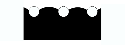
Figure 1: a).The ‘stones on a pillow’ model. AFP molecules, white circles, attach to a surface. b). Visualization of a surface of constant mean curvature. The size of the unit cell has been set to unity.

Since the adsorption is thought to be irreversible, the relationship between $n$, the density of AFP on the surface, and the concentration in solution must depend on the kinetics of the growth of the crystal, which we now model. In the simplest picture, the growth speed of the crystal boundary is proportional to the variation of the overall free energy of the system with respect to the normal displacement. In the small slope limit we take this to be $\delta h$. Then:

$$\dot{h}=-\Gamma\frac{\delta}{\delta h}\int\left[\gamma[1+|\nabla h|^{2}]^{1/2}+\Lambda\delta_{T}h\right]d^{2}\mathbf{r.}$$ (4)

The first term of the integrand is the surface energy, and the second is the difference of the bulk free energies of solid and liquid phases close to melting point. $\Gamma$ is a kinetic coefficient related to the rate of attachment of water molecules to the ice surface.

From the calculus of variations Goldstein et al. (2002) this equation is equivalent to:

$$\dot{h}=v_{o}\left[l_{0}\Delta h+\delta_{T}\right].$$ (5)

Here $v_{o}=\Gamma\Lambda$. This is a diffusion equation for $h$. The AFP’s are pinning centers for the surface, whose effect may be expressed as a set of boundary conditions:

$$\left.h\right|_{\left|\mathbf{r-r}_{i}\right|=b_{0}}=h_{i}.$$ (6)

Here $\mathbf{r}_{i}$ is the position of $i$-th AFP and $h_{i}$ is the height of its equatorial plane.

Suppose that the AFP’s in the water adsorb at random on the ice surface with rate, $k_{+}$, per unit area. The value of $h_{i}$ is the local position of the interface at the moment when the $i$-th AFP is adsorbed. The AFP’s effectively disappear when they get buried under the ice surface.

It will be useful to split $h\left(\mathbf{r}\right)$ into two contributions: $h\left(\mathbf{r}\right)=H+\phi\left(\mathbf{r}\right)$, where $H$ is the average height, and $\phi\left(\mathbf{r}\right)$ measures the small-scale variations. Suppose the AFP’s are randomly distributed with density, $n$. We choose $\phi$ to develop in time as:

$$\dot{\phi}=v_{o}l_{o}(\Delta\phi+4\pi\rho)$$ (7)

where $\rho=n<q>$ is chosen to make the surface neutral, and $<q>$ is the average charge. It is not hard to show that the time derivative in Eq. (7) for $\phi$ is small (the quasi-static limit). Thus:

$$\Delta\phi=-4\pi\left[\rho+\sum\limits_{i}q_{i}\delta\left(\mathbf{r-r}_{i}\right)\right].$$ (8)

The point charges account for the boundary conditions, Eq. (6). The values of $q_{i}$ are not fixed: as the interface moves, the charges vary from $0$ at the moment of creation to $-\chi b/2$, at which point the AFP is engulfed by ice.

Near an AFP, ($b<\left|\mathbf{r-r}_{i}\right|\ll 1/\sqrt{n}$), $\phi$ is dominated by the contribution of a single charge Jackson (1999):

$$\phi\left(\mathbf{r}\right)\simeq-q_{i}\log\pi\left(\mathbf{r-r}_{i}\right)^{2}n$$ (9)

Therefore:

$$q_{i}\simeq\frac{H-h_{i}}{\log\left(\pi nb^{2}\right)}<0$$ (10)

Since $|q|$ lies between 0 and $\chi b/2$, the ‘hole’ in the interface associated with the i^th AFP is of order $|q_{i}|\sim\chi b/4$. Subtracting Eq, (7) from Eq. (5), we find:

$$\dot{H}=v_{o}\left[\delta_{T}-4\pi l_{0}\rho\right].$$ (11)

Suppose the interface moves with constant speed $V$. Since each $h_{i}$ is fixed and $H$ changes uniformly with time, Eq. (10) implies that the magnitudes of individual point charges $q_{i}$ are uniformly distributed between $0$ and $-\chi b/2$, i.e. $\left\langle q\right\rangle=-\chi b/4$ and $\rho=nb/4$. This implies that $V=v_{o}(\delta_{T}-\pi\chi l_{o}bn)$.

The evolution of $n$ can be calculated by noting that its rate of increase is $k_{+}$, and that its rate of decrease is the rate that AFP’s are engulfed. Eq. (10) implies $\dot{q_{i}}=V/\log(\pi nb^{2})$. Since the $q_{i}$ are uniformly distributed we must have $dn/n=-\dot{q_{i}}dt/(\chi b/2)$. This gives:

$$\dot{n}=k_{+}-\frac{2nV}{\chi b\log\left(1/\pi nb^{2}\right)}.$$ (12)

In the steady state we put $\dot{n}=0$ in Eq. (12), and use the expression for $V$. Thus,

$$\frac{k_{+}}{v_{o}\delta_{T}}=\frac{n\left[2-n/n^{\ast}\right]}{\chi b\log\left(1/\pi nb^{2}\right)},$$ (13)

where $n^{\ast}=\delta_{T}\left(2\pi\chi bl_{0}\right)^{-1}$. The right hand side of this equation has a maximum for $n\approx n^{\ast}$. Thus, there is no constant speed solution unless the right hand side is small enough, i.e. for small enough $k_{+}$ or large enough $\delta_{T}$. The threshold $\delta_{T}^{*}$ obeys:

$$(\delta_{T}^{*})^{2}/\log(2\chi l_{0}/b\delta_{T}^{*})\simeq(\chi b)^{2}2\pi l_{0}k_{+}/v_{o}$$ (14)

To test our approximations, notably the quasi-static limit for $\phi$, we have performed a numerical simulation of Eqs. (5), (6), coupled to the random adsorption of AFP. Results on a $150\times 150$ square lattice, with each cell representing a single AFP, are shown in Figure 2. These results support our analysis. In fact, the transition from the steady growth to the arrested interface regime occurs at a somewhat lower adsorption rate $k_{+}$ than predicted. Since we have not performed a complete stability analysis of the steady-growth solution, Eq. (14) gives only an upper bound for the critical value of $k_{+}$. However, the discrepancy is rather small.

Beyond the transition point, growth stops. The resulting static interface must obey Eq. (5) with $\dot{h}=0$. Once again, we recover the Poisson equation, Eq. (1). After arrest, as Eq. (12) shows, $n$ increases as irreversible adsorption continues until limited by some aspect of surface chemistry that we have not considered in our model.

Real AFP’s are often anisotropic. In order to account for this, we assume that the region blocked is elliptical, with semi-major and semi-minor axes $a$ and $b$, respectively. The potential $h\left(x,y\right)$ can be found by conformal mapping Churchill and Brown (1990). Using this method, it is easy to show that Eq. (10) is replaced by: $H-h_{i}\simeq-q_{i}/\log\left(\pi n\left(a+b\right)^{2}/4\right)$. The slope of $h$ will reach its critical value near $x=\pm a$, and its maximum will be given by the radius of curvature of the ellipse, of order $b$. Thus $q_{\max}=\chi b/2$. With these changes, the left-hand side of Eq. (14) becomes

$$(\delta_{T}^{*})^{2}/\log(8\chi l_{0}b/(a+b)^{2}\delta_{T}^{*})$$ (15)

Eq. (14) involves $k_{+}/v_{o}$ The rate, $k_{+}$ is certainly proportional to the concentration, $C$, of AFP in solution: $k_{+}=v_{A}C$ where $v_{A}$ has the units of velocity. Therefore, $v_{A}/v_{o}$ is a parameter which we need to estimate.

In any experiment, soon after the adsorption process starts water near the ice surface is depleted of AFP. The thickness of the depletion layer depends on the diffusion coefficient $D$, as $\sqrt{Dt}$. That is, $k_{+}$ becomes time–dependent, and thus $v_{A}\simeq\sqrt{D/t}$. The same argument applies to the rate of crystallization itself: our estimate for $v_{o}$ fails as soon as the process is limited by thermal diffusion through a diffusive layer. Thus $v_{o}\simeq\sqrt{\kappa_{T}T/\Lambda t}$, where $\kappa_{T}$ is thermal conductivity of water. From the Einstein formula $D=k_{B}T/6\pi\eta b$:

$$v_{A}/v_{o}=\sqrt{\lambda/b}\sim 10^{-2}$$ (16)

where $\lambda=k_{B}\Lambda/6\pi\eta\kappa_{T}=1.2\times 10^{-10}$ cm. By combining Eqs. (14) and (16) we can write:

$$\delta_{T}^{*}\left[\log(2\chi l_{0}/b\delta_{T}^{*})\right]^{-1/2}\simeq\chi\sqrt{2\pi b^{3/2}l_{0}\lambda^{1/2}C},$$ (17)

For anisotropic AFP’s we must use Eq. (15) and also note that the longer axis, $a$, sets the hydrodynamic radius of the ellipsoidal particle. Its diffusion coefficient may be approximated by $D\approx k_{B}T\left(\beta+1\right)/6\pi\eta a$, where $\beta=\log((a+b)/2b)$ (typically, $\beta<2$). Thus

$$\delta_{T}^{*}[\log\left(2\chi l_{0}/b\delta_{T}^{*}\right)-2\beta]^{-1/2}$$

$$\simeq\chi b\left(\frac{\lambda}{a}\right)^{1/4}\sqrt{2\pi\left(\beta+1\right)l_{0}C},$$ (18)

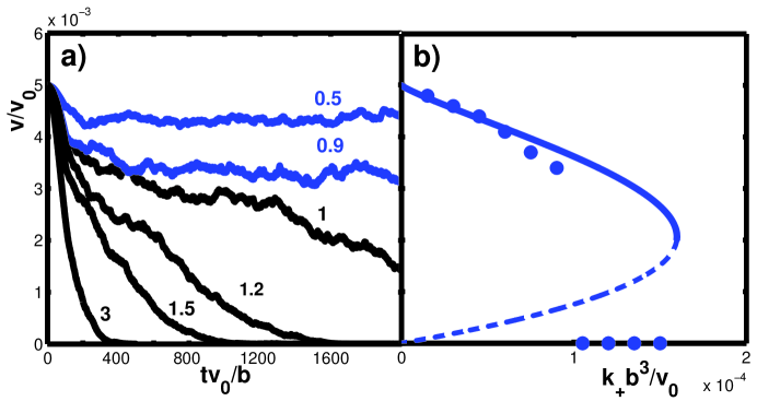
Figure 2: (a) Simulation results for the speed of the interface as a function of time, for various values of control parameter $k_{+}b^{3}/v_{0}$, ranging from $0.5\times 10^{-4}$ to $3\times 10^{-4}$. $\delta_{T}=0.005,\chi=1/(2\pi)$ (b) Speed in the steady state vs. reduced adsorption rate: comparison of simulation (points) with analytical result (line) given by Eq. 14.

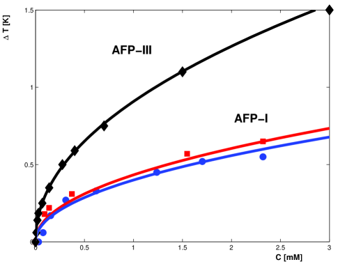
Figure 3: Comparison of theory to experiment for maximum undercooling  of water in the presence of  AFP–Type III (diamonds) and two modifications of AFP–Type I  (circles, squares).

Using these formulas, we have been able to fit the experimental data on natural AFP’s of two different classes: AFP–type I, and AFP–type III Chao et al. (1997); DeLuca et al. (1998). They have rather different architectures: AFP I is an $\alpha$-helical rod-like molecule which we model as a thin cylinder ($b=3.5\mathrm{\mathring{A}}$ , $a=25\mathrm{\mathring{A}}$), while AFP III has a more complicated globular structure, which we approximate as a sphere ($b=a=8\mathrm{\mathring{A}}$). Note that these lengths are derived from the known structures of the molecules, and therefore the only free parameter of our theory is $\chi$. The theoretical curves $\delta_{T}^{*}\left(C\right)$ are in excellent agreement with the experiments. The fact that values of the fitting parameter ( $\chi\simeq.25$ for AFP–I, and $\chi\approx.33$ for AFP–III) are physically reasonable and close to each other gives an additional support to our mechanism.

Note that according to Eq. (18), the activity is strongly dependent on the smaller dimension of the AFP. This may be useful for the design of synthetic AFP’s. E. g., by using ring–shaped molecules the $\delta_{T}^{*}$ could be increased since the effective size is set by the largest dimension, the radius of the ring, in this case. Our results are consistent with the measured $\delta_{T}^{*}\left(C\right)$ for Antifreeze Glycoproteins (AFGP). However, their molecular architecture and conformations are more complicated than those we have discussed, and their analysis would go beyond the scope of this work.

Finally, we can compare our results with the related problem of the motion of a pulled elastic interface in a medium with static obstacles to interface motion. This is of interest in the description of the kinetics of domain walls, charge density waves and flux lines in superconductors Kardar (1998). The interplay of long-range elastic coupling and local pinning results in a pinning-depinning transition at a critical value of the pulling force, and near the transition point, the average speed of the interface goes continuously to zero. Our model has pinning of the interface by the AFP molecules, and coupling due to surface tension, but the transition is discontinuous. The difference is that the AFP’s are not stationary. Their arrival at the interface is controlled by the adsorption process and is independent of the advance of the interface. To emphasize this difference, we call our model ‘kinetic pinning’. There should be a crossover between the static pinning and kinetic pinning if diffusion of the obstacles is taken into account.

We would like to thank Charles Knight and E. Brener for useful conversations. LMS acknowledges partial support by NSF grant No. DMS-0244419 and also the hospitality of the Kavli Institute for Theoretical Physics where this research was supported in part by NSF grant No. PHY99-07949.

References

- Knight and Wierzbicki (2001) C. A. Knight and A. Wierzbicki, Crys. Growth Des. 1, 439 (2001).
- Knight et al. (1991) C. A. Knight, C. C. Cheng, and A. L. Devries, Biophys. J. 59, 409 (1991).
- Duman (2001) J. G. Duman, Annu. Rev. Physiol. 63, 327 (2001).
- Fletcher et al. (2001) G. L. Fletcher, C. L. Hew, and P. L. Davies, Annu. Rev. Physiol. 63, 359 (2001).
- Devries (1983) A. L. Devries, Annu. Rev. Physiol. 45, 245 (1983).
- Knight et al. (2001) C. A. Knight, A. Wierzbicki, R. A. Laursen, and W. Zhang, Crys. Growth Des. 1, 429 (2001).
- Chao et al. (1997) H. M. Chao, M. E. Houston, R. S. Hodges, C. M. Kay, B. D. Sykes, M. C. Loewen, P. L. Davies, and F. D. Sonnichsen, Biochemistry 36, 14652 (1997).
- DeLuca et al. (1998) C. I. DeLuca, R. Comley, and P. L. Davies, Biophys. J. 74, 1502 (1998).
- Langer (1980) J. S. Langer, Rev. Mod. Phys. 52, 1 (1980).
- Goldstein et al. (2002) H. Goldstein, C. Poole, and J. Safko, Classical mechanics (Addison Wesley, San Francisco, 2002), 3rd ed.
- Jackson (1999) J. D. Jackson, Classical electrodynamics (Wiley, New York, 1999), 3rd ed.
- Churchill and Brown (1990) R. V. Churchill and J. W. Brown, Complex variables and applications (McGraw-Hill, New York, 1990), 5th ed.
- Kardar (1998) M. Kardar, Phys. Reps. 301, 85 (1998).