Power law load dependence of atomic friction

Abstract

We present a theoretical study of the dynamics of a tip scanning a graphite surface as a function of the applied load. From the analysis of the lateral forces, we extract the friction force and the corrugation of the effective tip-surface interaction potential. We find both the friction force and potential amplitude to have a power law dependence on applied load with exponent $\sim 1.6$. We interpret these results as characteristic of sharp undeformable tips in contrast to the case of macroscopic and elastic microscopic contacts.

It is well known that macroscopic friction is proportional to the applied load but the load dependence of atomistic friction is still under investigation and has been discussed in a limited number of experimental and theoretical works [1, 2, 3, 4, 5, 6, 7, 8]. Usually the load dependence is described by means of contact mechanics continuum theories [7, 8] which do not give information about the atomic interactions in the sliding contact region and assume a spherical tip. Moreover, it has been argued that, depending on the shape of the tip, power laws with different exponents can be found [7]. In this Letter, we present a detailed study of the load dependence of atomic-scale friction in the case of a sharp tip-surface contact, finding a power law dependence with exponent larger than one. We also show how the effective tip-surface potential energy barriers can be derived from force measurements, thus establishing a connection between friction and the interatomic potential. Recent works using noncontact mode Atomic Force Microscopy (AFM) have shown the possibility to reconstruct the tip-surface potential [9], but they lack the link between the corrugation of the potential and the friction force. The ideal way to achieve this goal is provided by a study of the load dependence.

We address the load dependence of friction by simulating the dynamics of a tip scanning a rigid monolayer graphite surface, extending to three dimensions ($3D$) the Tomlinson-like models of AFM [10]. Experimental evidences show that the tip usually cleaves small graphite flakes which remain attached to it [11]. Since the contact diameter between the tip and the surface can be very small we consider the limiting case in which the tip is formed by a single carbon atom connected via harmonic interactions with force constants $K_{x}$, $K_{y}$ and $K_{z}$ to a support moving along the scanning direction. The carbon atom of coordinates $(x,y,z)$ interacts with the graphite surface via the specific empirical potential $V_{TS}$ for graphite given by [12]:

$$V_{TS}=\sum_{j}\left[\theta(r_{0}-r_{Tj})V_{1}(r_{Tj})+\theta(r_{Tj}-r_{0})V_{2}(r_{Tj})\right]$$ (1)

where $\theta(r)$ is the Heaviside function, $r_{Tj}$ is the distance between the tip carbon atom and the $j-$th substrate atom and

$$V_{i}(r)=\epsilon_{i}\left(e^{-2\beta_{i}(r-r_{0})}-2e^{-\beta_{i}(r-r_{0})}\right)+v_{i}\qquad i=1,2$$ (2)

with $v_{1}=\epsilon_{1}-\epsilon_{2}$ and $v_{2}=0$. The values of the parameters are $r_{0}=0.371$ nm, $\epsilon_{1}=5.355$ meV, $\epsilon_{2}=2.614$ meV, $\beta_{1}=14.693$ nm^-1 and $\beta_{2}=21.029$ nm^-1. The tip support is moved with constant velocity $v_{scan}$ along the scanning line $x_{scan}=v_{scan}t$, $y_{scan}=$constant. We solve numerically the equations of motion in the constant force mode, i.e. we set $K_{z}=0$ and add a constant force $F_{load}$ in the downward $z$ direction, including also a damping term proportional to the atom velocity, which takes into account dissipation mechanisms:

$$\begin{array}[]{ccc}m\ddot{x}=-\frac{\partial V_{TS}}{\partial x}+K_{x}(x_{scan}-x)-m\eta\dot{x}\\ m\ddot{y}=-\frac{\partial V_{TS}}{\partial y}+K_{y}(y_{scan}-y)-m\eta\dot{y}\\ m\ddot{z}=-\frac{\partial V_{TS}}{\partial z}-F_{load}-m\eta\dot{z}\end{array}$$ (3)

We adopt an atomistic approach, assuming for $m$ the mass of a single carbon atom ($m=1.92\cdot 10^{-26}$ kg) and for the damping parameter $\eta=1$ ps^-1, which is a value appropriate for dissipation of energy and momentum at the atomic scale (see e.g. [13]). Here we show results for $K_{x}=K_{y}=1$ N/m which are typical values of AFM, whereas our scanning velocity $v_{scan}=0.4$ m/s is much higher than in experiments. Our choice of parameters makes the dynamics underdamped.

FIG. 1.: Tip-surface potential $V_{TS}$ as a function of the tip-surface distance $z$ with $x$ and $y$ coordinates taken as those of the hollow site (solid line). Points give the values of $V_{TS}$ at several positions along the actual trajectory as a function of the corresponding instantaneous value of $z$. Results for all indicated loads are obtained for simulations where the scanning direction is along a row of atoms ($y_{scan}=0.17$ nm).

The energetics underlying the tip motion for different loads is illustrated in Figs. 1 and 2. In Fig. 1 we present the tip-surface potential $V_{TS}$ as a function of the vertical tip-surface distance $z$, for in-plane coordinates corresponding to the position of the hollow site, on which we superimpose the values of $V_{TS}$ at actual positions of the tip during the simulations for different values of the load. The tip position probes the attractive part of the potential for low loads ($F_{load}=0.1$ nN) and moves closer and closer to the repulsive core of the substrate atoms for increasing loads. Clearly the whole tip-surface potential is probed by the motion of the tip for different loads, as suggested in Ref. [2]. In Fig. 2 we show the contour plots of $V_{TS}$ , calculated for $z$ given by the average value of the tip height at two values of the load. The scanning line $y_{scan}=0.17$ nm corresponds to scanning along a row of atoms. The actual trajectory is also reported: for the smaller load the motion follows a zig-zag-like pattern, while the trajectory acquires a one-dimensional stick-slip character for the higher load (see also [2]).

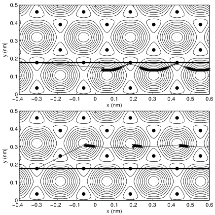
FIG. 2.: Contour plot of the potential $V_{TS}$ for $F_{load}=1$ nN (top) and $F_{load}=4$ nN (bottom) with $z$ fixed at the average value $<z>$ of the height obtained by the simulations ($<z>=0.25$ nm for $F_{load}=1$ nN and $<z>=0.2$ nm for $F_{load}=4$ nN). The minimum $V_{min}$ and the maximum $V_{max}$ of $V_{TS}$ are located respectively at the hollow site and on top of one atom. We show 10 contour lines between $V_{min}$ and $V_{max}$, separated by an energy interval $\Delta$. $V_{min}=123.5$ meV, $V_{max}=158.5$ meV and $\Delta=3.2$ meV for $F_{load}=1$ nN, while $V_{min}=774$ meV, $V_{max}=1.01$ eV and $\Delta=23.7$ meV for $F_{load}=4$ nN. The horizontal thick solid line indicates the scanning direction ($y_{scan}=0.17$ nm), while the crosses are points along the actual atomic trajectory taken every $4$ ps.

Fig. 3 presents typical force plots as a function of $x_{scan}$ and $x$ [14] for $F_{load}=2$ nN and $F_{load}=4$ nN. The sawtooth behavior characteristic of stick-slip motion is determined by the competition between the elastic force ${\bf F}_{el}$ and the force ${\bf F}_{TS}$ due to the tip-surface potential $V_{TS}$. Elastic energy, accumulated in the spring, is counterbalanced by the substrate attraction, until, suddenly, the tip slips to another minimum. Therefore, while sticking, ${\bf F}_{el}$ mirrors ${\bf F}_{TS}$. This fact can be used to derive $V_{TS}$ itself. The solid lines in Fig. 3 represent the lateral force along the scanning direction, $F_{el}^{x}$, as obtained by our simulations. Increasing the load enhances the sawtooth behavior of the stick-slip motion and gives rise to a larger initial sticking region, often observed experimentally (see e.g. [15]).

As shown in Fig. 2 the actual trajectory does not necessarily follow the scanning line so that the potential energy landscape during the motion is not known a priori. However, we can extract the effective value of the energetic barrier $V_{0}$ for a given $F_{load}$ directly from the force plots. By assuming a sinusoidal shape of $F_{TS}$ [5, 16] and noting that $F_{TS}$ should average to zero for a periodic substrate, we can reconstruct $F_{TS}^{x}$.

FIG. 3.: Lateral forces along the scanning direction for $F_{load}=2$ nN [(a),(c)] and $F_{load}=4$ nN [(b),(d)], plotted as a function of $x_{scan}$ [(a),(b)] and $x$ [(c),(d)], for $y_{scan}=0.17$ nm. Solid lines are the elastic forces $F_{el}^{x}$ obtained by simulations, while the dashed lines in (c) and (d) are static calculations of the tip-surface force (with reverted sign) $-F_{TS}^{x}$ at $(y,z)$ determined by averaging $y(t)$ and $z(t)$ given by the dynamics. The dotted lines in (a), (b) give the slope $K_{eff}$ of the sticking part ($K_{eff}=0.78$ N/m for $F_{load}=2$ nN and $K_{eff}=0.89$ N/m for $F_{load}=4$ nN).

Then, the tip-surface potential $V_{TS}$ is simply given, up to a constant, by integrating $F_{TS}^{x}$:

$$V_{TS}(x)=-\int F_{TS}^{x}dx=\frac{V_{0}}{2}\sin\left(\frac{2\pi x}{a}\right)+const.$$ (4)

with $V_{0}=F_{0}a/(2\pi)$, where $a$ and $F_{0}$ are the period and the amplitude of $F_{TS}$. In Figs. 3(c)-(d) we show $-F_{TS}^{x}$ (dashed lines) obtained by static calculations for $(y,z)$ determined by averaging $y(t)$ and $z(t)$ given by the dynamics. Indeed, $-F_{TS}^{x}$ follows the sticking parts of $F_{el}^{x}$ quite well. The first stick signal, of larger amplitude, is the most suitable to estimate the amplitude of $F_{TS}^{x}$.

FIG. 4.: Load dependence of the energy barrier (a) and of the friction force (b) for $y_{scan}=0.17$ nm. Inset of (b): relation between friction force and energy barrier. The solid circles are the result of the simulations and the dashed lines are power law fits, as explained in the text.

The resulting dependence of the energy barrier $V_{0}$ on the load is shown in Fig. 4(a). An increase of $V_{0}$ with $F_{load}$ has also been found experimentally [2, 17]. The dashed line in Fig. 4(a) is a power law fit to the numerical data with exponent $\sim 1.6$. Fig. 4(b) illustrates the lateral friction force $F_{fric}$, obtained as the mean value of the instantaneous lateral force $F_{el}^{x}$, as a function of $F_{load}$. Also these data can be fitted by a power law with exponent $\sim 1.6$. Thus, the linear relation between macroscopic friction and load does not hold at the microscopic level. Moreover, the exponent is different from the $2/3$ expected for a Hertzian contact [7, 8]. As pointed out in Ref. [7] even a small deviation from the spherical shape of the tip can be responsible for a change in the power law exponent. We conjecture that exponents larger than one are characteristic of sharp, undeformable tip-surface contacts. Note that, since the power law exponents for $V_{0}$ and $F_{fric}$ as a function of $F_{load}$ are very close, an approximately linear relation between $F_{fric}$ and $V_{0}$ is recovered (see inset of Fig. 4(b)), indicating a direct link between atomistic friction and energy barriers for diffusion.

In conclusion, we have presented a theoretical study of the $3D$ dynamics of a tip scanning a graphite surface with realistic interactions as a function of the applied load. We predict a power law behavior with exponent $\sim 1.6$ for the friction force as a function of applied load, at variance with macroscopic behavior. The study of the load dependence establishes a direct linear relation between friction and potential corrugation in the contact region.

This work was supported by the Stichting Fundamenteel Onderzoek der Materie (FOM) with financial support from the Nederlandse Organisatie voor Wetenschappelijk Onderzoek (NWO). The authors wish to thank Elisa Riedo, Jan Los, Sylvia Speller, Sergey Krylov and Jan Gerritsen for useful and stimulating discussions.

REFERENCES

- [1] S. Fujisawa, E. Kishi, Y. Sugawara and S. Morita, Phys. Rev. B 52, 5302 (1995).
- [2] S. Fujisawa, K. Yokoyama, Y. Sugawara and S. Morita, Phys. Rev. B 58, 4909 (1998).
- [3] M. Ishikawa, S. Okita, N. Minami and K. Miura, Surf. Sci. 445, 488 (2000).
- [4] N. Sasaki, M. Tsukada, S. Fujisawa, Y. Sugawara, S. Morita and K. Kobayashi, Phys. Rev. B 57, 3785 (1998).
- [5] W. Zhong and D. Tománek, Phys. Rev. Lett. 64, 3054 (1990).
- [6] M. R. Sørensen, K. W. Jacobsen and P. Stoltze, Phys. Rev. B 53, 2101 (1996).
- [7] U. D. Schwarz, O. Zwörner, P. Köster and R. Wiesendanger, Phys. Rev. B 56, 6987 (1997).
- [8] M. Enachescu, R. J. A. van den Oetelaar, R.W. Carpick, D. F. Ogletree, C. F. J. Flipse and M. Salmeron, Phys. Rev. Lett. 81, 1877 (1998).
- [9] H. Hölscher, W. Allers, U. D. Schwarz, A. Schwarz and R. Wiesendanger, Phys. Rev. Lett. 83, 4780 (1999); Phys. Rev. B 62, 6967 (2000); H. Hölscher, A. Schwarz, W. Allers, U. D. Schwarz and R. Wiesendanger, ibid. 61, 12678 (2000); U. D. Schwarz, H. Hölscher and R. Wiesendanger, ibid. 62, 13089 (2000).
- [10] D. Tománek, W. Zhong and H. Thomas, Europhys. Lett. 15, 887 (1991); N. Sasaki, K. Kobayashi and M. Tsukada, Phys. Rev. B 54, 2138 (1996); H. Hölscher, U. D. Schwarz and R. Wiesendanger, Surf. Sci. 375, 395 (1997); Y. Sang, M. Dubé and M. Grant, Phys. Rev. Lett. 87, 174301 (2001).
- [11] M. Dienwiebel, Ph.D. Thesis, University of Leiden, 2003.
- [12] J. H. Los and A. Fasolino, Comp. Phys. Comm. 147, 178 (2002); Phys. Rev. B 68, 024107 (2003).
- [13] R. Guantes, J. L. Vega, S. Miret-Artés and E. Pollak, J. Chem. Phys. 119, 2780 (2003); H. Xu and I. Harrison, J. Phys. Chem. B 103, 11233 (1999).
- [14] Experimental force plots data are often given as a function of . However, since , it is straightforward to rewrite the data as .
- [15] S. Morita, S. Fujisawa and Y. Sugawara, Surf. Sci. Rep. 23, 1 (1996).
- [16] S. H. Ke, T. Uda, R. Pérez, I. S̆tich and K. Terakura, Phys. Rev. B 60, 11631 (1999).
- [17] E. Riedo, E. Gnecco, R. Bennewitz, E. Meyer and H. Brune, Phys. Rev. Lett. 91, 084502 (2003).