Magic Angle Effects and AMRO as Dimensional Crossovers

Abstract

It is shown that interference effects between velocity and density of states, which occur as electrons move along open orbits in the extended Brillouin zone, result in a change of wave functions dimensionality at Magic Angle (MA) directions of a magnetic field. In a particular, we demonstrate that these $1D\rightarrow 2D$ dimensional crossovers result in the appearance of sharp minima in a resistivity component $\rho_{zz}(H,\alpha)$, perpendicular to conducting layers, which explains the main qualitative features of MA and Angular Magneto-Resistance Oscillations (AMRO) phenomena observed in low-dimensional conductors (TMTSF)₂X, (DMET-TSeF)₂X, and $\alpha$-(BEDT-TTF)₂MHg(SCN)₄.

PACS numbers: 74.70.Kn, 73.43-f, 75.30.Fv

Low-dimensional organic conductors (TMTSF)₂X (X = PF₆, ClO₄, …), (DMET-TSeF)₂X (X = AuCl₂, …), and $\alpha$-(BEDT-TTF)₂MHg(SCN)₄ (M=K, Tl, …) exhibit a number of unconventional angular magnetic oscillations [1-24] related to open quasi-one-dimensional (Q1D) sheets of Fermi surface (FS) in a metallic phase [1-3],

$$\epsilon^{\pm}({\bf p})=\pm v_{F}\ (p_{x}\mp p_{F})-2t_{b}\cos(p_{y}b^{*})-2t_{c}\cos(p_{z}c^{*})\ ,\ \ \ \ p_{F}v_{F}\gg t_{b}\gg t_{c}\ ,$$ (1)

where $+(-)$ stands for the right (left) sheet of the FS; $v_{F}$ and $p_{F}$ are the Fermi velocity and Fermi momentum along conducting ${\bf x}$-axis, respectively; $t_{b}$ and $t_{c}$ are the overlapping integrals between conducting chains; $\hbar\equiv 1$. Most unconventional angular oscillations in a metallic phase - the so-called Danner-Kang-Chaikin oscillations [17], the third angular effect [18-20], and the interference commensurate (IC) oscillations [20,21] - have been explained in term of Fermi liquid (FL) approach to anisotropic Q1D spectrum (1) (see Ref. [17], Ref. [25], and Refs. [26,27], correspondingly).

On the other hand, despite the fact that all experimentally observed ”magic angle” (MA) phenomena [5-16] and AMRO [22-24] are related to MA directions [4,28,35] of a magnetic field,

$$\tan\alpha=(n/m)\ (b^{*}/c^{*})\ ,\ \ \ \ {\bf H}=(0,H\sin\alpha,H\cos\alpha)\ ,$$ (2)

(where n and m are integers) corresponding to periodic electron orbits in $(p_{y},p_{z})$-plane [4,35], there is no good agreement between the numerous theories of MA phenomena [28-39] and experiments [5-16] in a metallic phase. There exist even experimental evidences that, although some MA effects in a metallic phase [7,16] are of FL origin, the others [3,12-14] may significantly break FL picture. So far, the best qualitative agreements have been achieved between the prediction of Ref.[4] and the minima in onset magnetic fields for field-induced spin-density-wave phases observed at MA directions of the field (2) [8,37].

The goal of our Letter is to demonstrate that electron wave functions, corresponding to open FS in a realistic tight-binding model of Q1D spectrum with electron hoping only between the neighboring atomic sites,

$$\epsilon^{\pm}({\bf p})=\pm v_{x}(p_{y})\ [p_{x}\mp p_{x}(p_{y})]-2t_{c}\cos(p_{z}c^{*})\ ,\ \ \ \ \ p_{x}(p_{y})=p_{F}+2t_{b}\cos(p_{y}b^{*})/v_{F}\ ,$$ (3)

change their dimensionality from $1D$ to $2D$ at MA directions of a magnetic field (2) with $m=1$:

$$\tan\alpha=n\ (b^{*}/c^{*})\ .$$ (4)

In particular, we show that, in the absence of Landau level quantization for open FS (3), the other quantum effects in a magnetic field - Bragg reflections result in $1D\rightarrow 2D$ dimensional crossovers at MA directions of the field (4).

In other words, electron wave functions, which are localized on the conducting chains at arbitrary directions of a magnetic field [4,40], become $2D$ (i.e., localized on some planes) at the MA directions of a magnetic field (4). As shown below, non-trivial physical origin of these $1D\rightarrow 2D$ dimensional crossovers is related to the interference effects between velocity component along z-axis, $v_{z}(...)$, perpendicular to conducting (x,y)-planes, and the density of states, $v_{x}(...)$. These interference effects occur as electrons move along open FS (3) in the extended Brillouin zone and are qualitatively different from that responsible for IC oscillations [27,26]. Using this finding, we demonstrate that it is possible to explain the appearance of MA [7,13,15,16] and AMRO [22-24] minima in resistivity component $\rho_{zz}(H,\alpha)$, perpendicular to conducting planes in (TMTSF)₂X, (DMET-TSeF)₂X, and $\alpha$-(BEDT-TTF)₂MHg(SCN)₄ compounds in the framework of FL approach. We also hope that suggested in this Letter $1D\rightarrow 2D$ dimensional crossovers will be the key points in further FL and non-Fermi-liquid (n-FL) theories of more complex MA phenomena.

At first, let us discuss how $1D\rightarrow 2D$ dimensional crossovers can lead to the appearance of MA minima in $\rho_{zz}(H,\alpha)$ using qualitative arguments. For electrons localized on conducting ${\bf x}$-chains [4,40], it is natural to expect that conductivity component $\sigma_{zz}(H,\alpha)$ is zero in the absence of impurities (i.e., at $1/\tau=0$) and decays as $1/\tau^{2}\omega^{2}_{c}(H)\sim 1/H^{2}$ at high fields. [Here, $\omega_{c}(H)$ is one of the cyclotron frequencies related to electron motion along open FS (3), $\tau$ is an electron relaxation time.] If, at MA directions of the field (4), electron wave functions become delocalized, then $\sigma_{zz}(H,\alpha)$ is expected to have similarities with conductivity of free electrons at $H=0$. Therefore, $\sigma_{zz}(H,\alpha)$ has to saturate at high magnetic fields and is expected to be proportional to $\tau$. Below, we demonstrate that this qualitatively different behavior of $\sigma_{zz}(H,\alpha)$ at MA directions (4) is indeed responsible for the appearance of MA minima in $\rho_{zz}(H,\alpha)$.

To develop a quantitative theory, we make use of the Peierls substitution method [41] for open electron spectrum [42,4]: $p_{x}\rightarrow-id/dx,\ p_{y}\rightarrow p_{y}-(e/c)A_{y},\ p_{z}\rightarrow p_{z}-(e/c)A_{z}$. It is convenient to chose vector potential of the magnetic field (2) in the form ${\bf A}=(0,\ Hx\cos\alpha,\ -Hx\sin\alpha)$, where Hamiltonian (3) in the vicinity of $p_{x}\simeq p_{F}$ can be expressed as

$${\hat{\epsilon}^{+}({\bf p})}=v_{x}\biggl{[}p_{y}b^{*}-\frac{\omega_{b}(\alpha)x}{v_{F}}\biggl{]}\biggl{(}-i\frac{d}{dx}-p_{x}\biggl{[}p_{y}b^{*}-\frac{\omega_{b}(\alpha)x}{v_{F}}\biggl{]}\biggl{)}-2t_{c}\cos\biggl{[}p_{z}c^{*}+\frac{\omega_{c}(\alpha)x}{v_{F}}\biggl{]}\$$ (5)

with

$$\omega_{b}(\alpha)=eHv_{F}b^{*}\cos\alpha/c\ ,\ \ \ \ \omega_{c}(\alpha)=eHv_{F}c^{*}\sin\alpha/c\$$ (6)

being cyclotron frequencies of electron motion along ${\bf y}$-axis and ${\bf z}$-axis, respectively.

An important difference between Hamiltonian (5) and the Hamiltonians [27,42,4] studied so far is that velocity component along the conducting ${\bf x}$-chains [i.e., operator of the density of states, ${\hat{v}_{x}(...)}$] depends on $p_{y}$ and $x$. Although in this case the operators ${\hat{v}_{x}(...)}$ and $d/dx$ do not commute, nevertheless one can ignore this fact if the quasi-classical parameter

$$4t_{c}/\omega_{b}(\alpha)\gg 1\ .$$ (7)

It is possible to make sure that, if one represents electron wave functions in the form

$$\Psi_{\epsilon}(x,p_{y},p_{z})=\exp\biggl{(}i\int^{x}_{0}p_{x}\biggl{[}p_{y}b^{*}-\frac{\omega_{b}(\alpha)u}{v_{F}}\biggl{]}\ du\biggl{)}\ \psi_{\epsilon}(x,p_{y},p_{z})\ ,$$ (8)

then the solutions of the Schrodinger equation for Hamiltonian (5) can be written as

$$\psi_{\epsilon}(x,p_{y},p_{z})=\frac{1}{\sqrt{v_{x}[p_{y}b^{*}-\frac{\omega_{b}(\alpha)x}{v_{F}}]}}\ \exp\biggl{(}i\int^{x}_{0}\frac{\epsilon\ du}{v_{x}[p_{y}b^{*}-\frac{\omega_{b}(\alpha)u}{v_{F}}]}\biggl{)}\exp\biggl{(}2it_{c}\int^{x}_{0}\frac{\cos[p_{z}c^{*}+\frac{\omega_{c}(\alpha)u}{v_{F}}]}{v_{x}[p_{y}b^{*}-\frac{\omega_{b}(\alpha)u}{v_{F}}]}du\biggl{)}.$$ (9)

[In Eq.(9), we normalize wave functions by the standard condition, $\int\psi_{\epsilon_{1}}(x)\psi_{\epsilon_{2}}(x)\ dx=\delta(\epsilon_{1}-\epsilon_{2})$, and make use of the inequality (7)].

Let us demonstrate that suggested in the Letter $1D\rightarrow 2D$ dimensional crossovers directly follow from Eq.(9). It is possible to prove that in the limiting case, where $v_{x}[...]=v_{F}=const$, wave functions (8,9) are always localized on conducting ${\bf x}$-chains (see Refs. [40,4]). Below, we show that an account of $p_{y}$- and $x$-dependences of the density of states, $v_{x}[p_{y}b^{*}-\omega_{b}(\alpha)x/v_{F}]$, in Eq. (9) lead to de-localization crossovers at MA directions of a magnetic field (4). For this purpose, we calculate $z$-dependence of electron wave functions at $z=Nc^{*}$ (where $N$ is an integer) by taking a Fourier transformation of the second exponential function in Eq.(9):

$$\Phi(x,p_{y},z=Nc^{*})=\int_{0}^{2\pi}\ \frac{d\ p_{z}}{2\pi}\exp(ip_{z}Nc^{*})\ \exp\biggl{(}2it_{c}\int^{x}_{0}\frac{\cos[p_{z}c^{*}+\frac{\omega_{c}(\alpha)u}{v_{F}}]}{v_{x}[p_{y}b^{*}-\frac{\omega_{b}(\alpha)u}{v_{F}}]}du\biggl{)}\ .$$ (10)

After straightforward calculations, $z$-dependence of electron wave-functions (10) can be expressed as

$$\Phi(x,p_{y},z=Nc^{*})=\exp[-i\phi(x,\alpha,p_{y})N]\ J_{-N}\biggl{[}2t_{c}\sqrt{I^{2}_{1}(x,\alpha,p_{y})+I^{2}_{2}(x,\alpha,p_{y})}\biggl{]}\ ,$$ (11)

where

$$I_{1}(x=2\pi M_{0}v_{F}/\omega_{b}(\alpha),\alpha,p_{y})=\sum^{M_{0}}_{M=0}\int^{2\pi v_{F}/\omega_{b}(\alpha)}_{0}\ \frac{\cos\biggl{[}\frac{\omega_{c}(\alpha)u}{v_{F}}+2\pi M\frac{\omega_{c}(\alpha)}{\omega_{b}(\alpha)}\biggl{]}}{v_{x}(p_{y}b^{*}-\omega_{b}(\alpha)\ u/v_{F})}\ du$$

$$I_{2}(x=2\pi M_{0}v_{F}/\omega_{b}(\alpha),\alpha,p_{y})=\sum^{M_{0}}_{M=0}\int^{2\pi v_{F}/\omega_{b}(\alpha)}_{0}\ \frac{\sin\biggl{[}\frac{\omega_{c}(\alpha)u}{v_{F}}+2\pi M\frac{\omega_{c}(\alpha)}{\omega_{b}(\alpha)}\biggl{]}}{v_{x}(p_{y}b^{*}-\omega_{b}(\alpha)\ u/v_{F})}\ du\ ,$$ (12)

with $J_{N}(...)$ being the Bessel function [43]; $M_{0}$ is an integer. According to the Bessel functions theory [43], $J_{N}(Z)$ is an oscillatory function of the variable $N$ at $N<|Z|$, whereas it decays exponentially with $N$ at $N>|Z|$. Thus, one can conclude that wave functions (10)-(12) are extended along $z$-direction if at least one of the functions $I_{i}(...)$ in Eq.(12) is not restricted [i.e., if $|I_{i}(M_{0},\alpha,p_{y})|\rightarrow\infty$ as $M_{0}\rightarrow\infty$]. In the opposite case, where both functions $I_{i}(...)$ ($i=1,2$) are restricted by the conditions $|I_{1}(M_{0},\alpha,p_{y})|,|I_{2}(M_{0},\alpha,p_{y})|<I_{max}$, electron wave functions (10)-(12) exponentially decay with the variable $z$ at $|z=Nc^{*}|\geq 2I_{max}$.

Note that functions (12) are written in the form of summations of infinite number of electron waves corresponding to electron quasi-classical motion in different Brillouin zones in the extended Brillouin zone picture. Therefore, the physical meaning of summations in Eq.(12) is related to the interference effects between velocity component along ${\bf z}$-axis, $v_{z}=-2t_{c}c^{*}\sin(p_{z}c^{*}+\omega_{c}(\alpha)u/v_{F})$, and the density of states, $v_{x}[p_{y}b^{*}-\omega_{b}(\alpha)u/v_{F}]$, which occur due to Bragg reflections as electron move in a magnetic field along open orbits. As it is seen from Eq.(12), angular dependent phase difference between electron waves, $2\pi M\omega_{c}(\alpha)/\omega_{b}(\alpha)$, is an integer number of $2\pi$ only at MA directions (4) of a magnetic field (2), where $\omega_{c}(\alpha)=n\ \omega_{b}(\alpha)$, with $n$ being an integer. Therefore, one comes to the conclusion: at arbitrary direction of a magnetic field, the destructive interference effects in Eq.(12) result in exponential decay of electron wave functions (10)-(12) along ${\bf z}$-axis, whereas, at MA directions, the constructive interference effects cause to delocalization of wave functions along ${\bf z}$-axis.

To calculate conductivity $\sigma_{zz}(H,\alpha)$, let us introduce the quasi-classical operator of the velocity component $v_{z}(...)$ in a magnetic field [27]:

$${\hat{v}_{z}(p_{z},x)}=-v^{0}_{z}\sin[p_{z}c^{*}+\omega^{0}_{c}(\alpha)x/v_{F}]\ ,\ \ \ \ v^{0}_{z}=2t_{c}c^{*}.$$ (13)

Since wave functions (8)-(10) and the velocity operator (13) are known, one can calculate $\sigma_{zz}(H,\alpha)$ by means of Kubo formalism. As a result, one obtains

$$\sigma_{zz}(H,\alpha)\sim\biggl{<}\frac{1}{v_{x}(p_{y})}\ \int^{0}_{-\infty}\ d(b^{*}u)\ \frac{\cos[n(\alpha)b^{*}u]}{\omega_{b}(p_{y}+u,\alpha)}\exp\biggl{[}-\int^{0}_{u}\frac{d(b^{*}u_{1})}{\tau\omega_{b}(p_{y}+u_{1},\alpha)}\biggl{]}\biggl{>}_{p_{y}}\ ,$$ (14)

where

$$\omega_{b}(p_{y},\alpha)=\omega_{b}(\alpha)\ [v_{x}(p_{y})/v_{F}]\ ,\ \ \omega_{c}(p_{y},\alpha)=\omega_{c}(\alpha)\ [v_{x}(p_{y})/v_{F}]\ ,\ \ n(\alpha)=\omega_{c}(\alpha)/\omega_{b}(\alpha)\ ,$$ (15)

$<...>_{p_{y}}$ stands for avereging procedure over variable $p_{y}$.

After straightforward but rather complicated integrations, Eq.(14) can be rewritten as

$$\frac{\sigma_{zz}(H,\alpha)}{\sigma_{zz}(0)}=\frac{1}{1+h^{2}_{c}(H)}\ - h^{2}_{c}(H)\ \int^{0}_{-\infty}\ du\ \exp(u)\cos[h_{c}(H)u]$$

$$\times\biggl{<}\exp\biggl{[}\int^{u}_{0}f[y+u_{1}h_{b}(H)]du_{1}\biggl{]}-1\biggl{>}_{y}\ ,$$

$$f(y)=v_{F}/v_{x}(y)-1,\ \ \ h_{b}(H)=\omega_{b}(\alpha)\tau\ ,\ \ \ h_{c}(H)=\omega_{c}(\alpha)\tau\ .$$ (16)

Since in Q1D case $\rho_{zz}(H,\alpha)\simeq 1/\sigma_{zz}(H,\alpha)$, Eq.(16) solves a problem to define $\rho_{zz}(H,\alpha)$ for electrons with open spectrum (3) in an inclined magnetic field (2) [44].

To make our results more intuitive, we consider the most important limiting case - a so-called clean limit, where $\omega_{c}(\alpha)\ \tau\gg 1$. In this case, Eq.(16) can be significantly simplified:

$$\frac{\sigma_{zz}(H,\alpha)}{\sigma_{zz}(0)}= \biggl{[}\frac{1}{1+[\omega_{c}(\alpha)\tau]^{2}}-\tan^{2}\alpha\ \biggl{(}\frac{c^{*}}{2b^{*}}\biggl{)}^{2}\sum^{\infty}_{n=1}\ \frac{A^{2}_{n}}{n^{2}}\ \biggl{(}\frac{2}{1+[\omega_{c}(\alpha)\tau]^{2}}$$ (17)

$$-\frac{1}{1+[\omega_{c}(\alpha)-n\omega_{b}(\alpha)]^{2}\tau^{2}}-\frac{1}{1+[\omega_{c}(\alpha)+n\omega_{b}(\alpha)]^{2}\tau^{2}}\biggl{)}\biggl{]}$$

where where $A_{n}$ are the Fourier coefficients of function $f(y)=v_{F}/v_{x}(y)-1$:

$$A_{N}=\frac{1}{\pi}\int^{+\pi}_{-\pi}\ f(y)\cos(Ny)\ dy\ .$$ (18)

Eq.(17) directly demonstrates MA maxima in $\sigma_{zz}(H,\alpha)$ [i.e., minima in $\rho_{zz}(H,\alpha)$] related to minima of denominators which occur at $\omega_{c}(\alpha)=n\omega_{b}(\alpha)$ [i.e., at MA directions of the field (4)]. In Fig.1, we present numerical simulations of Eqs.(17),(18) for three qualitatively different variants of Q1D spectra (3) corresponding to (TMTSF)₂PF₆, $\alpha$-(BEDT-TTF)₂MHg(SCN)₄, and (TMTSF)₂ClO₄ conductors. As it is seen, (TMTSF)₂PF₆ exhibits only one MA minimum, whereas the last two compounds exhibit several MA minima with large indexes $n$ in Eq.(4). We stress that this qualitative feature as well as a doubling of a period of MA minima in the case of (TMTSF)₂ClO₄ are in a good agreement with the existing experimental data [5,7,13,16,22].

We point out that the existing alternative model to describe MA and AMRO effects in $\rho_{zz}(H,\alpha)$ - a so-called Osada model [30], which is very important from methodological and historical points of view, in our opinion, does not have a direct physical meaning. The reason is that the transfer integrals $t_{n,m}$ in Ref.[30] are expected to be exponentially small in the framework of a realistic tight-binding model [1] of low-dimensional electron spectra. Moreover, as it follows from Eq.(17), a hypothesis [30] that it is possible to introduce some ”effective transfer integrals”, $t_{n,m}$, in a linearized electron spectrum (1) and to use such linearized spectrum while calculating $\rho_{zz}(H,\alpha)$ is incorrect. Indeed, weighting factors in Eq.(17) depend on magnetic field orientation (i.e., on $\tan\alpha$) and, thus, their physical meanings are completely different from some ”effective transfer integrals”, $t_{n,m}$, postulated in Ref.[30].

In conclusion, we hope that $1D\rightarrow 2D$ dimensional crossovers suggested in the Letter will be key points in further theories describing more complicated MA phenomena. In this connection, we point out that there exist three main scenarios for MA phenomena: FL one [4,28-33] based on Gor’kov [42,45] and Chaikin [46] approach to Q1D conductors, weak n-FL one [28,35], where electron-electron scattering processes depend on a magnetic field, and n-FL Princeton scenario [12-14,34,36], where MA direction of a magnetic field correspond to FL versus n-FL crossovers. Very recently, two novel exotic mechanisms [39,47] have been suggested to account for MA and AMRO effects.

This work was supported in part by National Science Foundation, grant number DMR-0076331, the Department of Energy, grant number DE-FG02-02ER63404, and by the INTAS grants numbers 2001-2212 and 2001-0791. One of us (AGL) is thankful to N.N. Bagmet and E.V. Brusse for useful discussions.

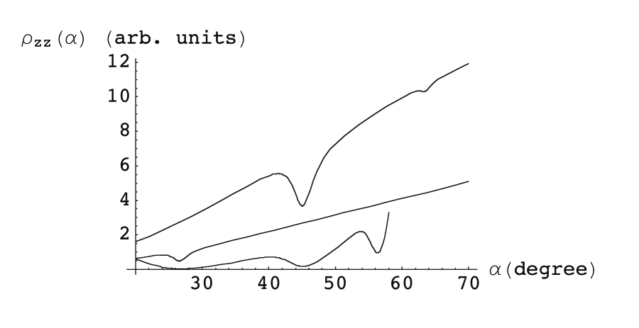
Figure 1: Resistivity component $\rho_{zz}(\alpha)=1/\sigma_{zz}(\alpha)$, perpendicular to conducting layers, calculated by means of Eqs.(17),(18),(5). For $\alpha$-(BEDT-TTF)₂MHg(SCN)₄ (lower curve) and (TMTSF)₂PF₆ (middle curve) conductors, we use model electron spectrum $\epsilon(p_{x},p_{y},p_{z})=2t_{a}\cos(p_{x}a/2)+2t_{b}\cos(p_{y}b^{*})+2t_{c}\cos(p_{z}c^{*})$ [1] with weak, $t_{a}/t_{b}\simeq 3$, and strong, $t_{a}/t_{b}=8.5$ [27], Q1D anisotropies, respectively. For (TMTSF)₂ClO₄ conductor (upper curve), we take into account anion ordering [1] and, thus, use the spectrum $\epsilon(p_{x},p_{y},p_{z})=2t_{a}\cos(p_{x}a/2)+\sqrt{[2t_{b}\cos(p_{y}b)]^{2}+\Delta^{2}}+2t_{c}\cos(p_{z}c)$ [1] with $t_{a}/t_{b}=8.5$ and $\Delta=0.2t_{b}$. In all three cases, we use the value $\omega_{b}(0)\tau=15$.

References

- (1) T. Ishiguro, K. Yamaji, and G. Saito, Organic Superconductors (Second Edition, Springer-Verlag, Heidelberg, 1998).
- (2) See review articles in J. Phys. I (France) 6 (1996) and references therein.
- (3) See recent review S.E. Brown, M.J. Naughton, I.J. Lee, E.I. Chashechkina, and P.M. Chaikin in More is Different, N.P. Ong and R.N. Bhatt Eds. (Princeton University Press, Princeton, 2001) and references therein.
- (4) A.G. Lebed, Pis’ma Zh. Eksp. Teor. Fiz. 43, 137 (1986) [JETP Lett. 43, 174 (1986)].
- (5) M.J. Naughton, O.H. Chung, M. Chaparala, X. Bu, and P. Coppens, Phys. Rev. Lett. 67, 3712 (1991); M.J. Naughton, O.H. Chung, L.Y. Chiang, and J.S. Brooks, Mat. Res. Soc. Symp. Proc. 173, 257 (1990).
- (6) G.S. Boebinger, G. Montambaux, M.L. Kaplan, R.C. Haddon, S.V. Chichester, and L.Y. Chiang, Phys. Rev. Lett. 64, 591 (1990).
- (7) T. Osada, A. Kawasumi, S. Kagoshima, N. Miura, and G. Saito, Phys. Rev. Lett. 66, 1512 (1991).
- (8) W. Kang, S.T. Hannahs, and P.M. Chaikin, Phys. Rev. Lett. 69 2827 (1992).
- (9) K. Behnia, M. Ribault, and C. Lenoir, Europhys. Lett. 25, 285 (1994).
- (10) W. Kang, S.T. Hannahs, and P.M. Chaikin, Physica B 201, 442 (1994).
- (11) K. Oshima, H. Okuno, K. Kato, R. Maruyama, R. Kato, A. Kobayashi, and H. Kobayashi, Synth. Metals 70, 861 (1995).
- (12) E.I. Chashechkina and P.M. Chaikin, Phys. Rev. Lett. 80, 2181 (1998).
- (13) E.I. Chashechkina and P.M. Chaikin, Phys. Rev. B 65, 012405 (2002).
- (14) W. Wu, I. J. Lee, and P. M. Chaikin, Phys. Rev. Lett. 91, 056601 (2003)
- (15) H. Kang, Y. J. Jo, S. Uji, and W. Kang, Phys. Rev. B 68, 132508 (2003).
- (16) H. Kang, Y. J. Jo, W. Kang, Phys. Rev. B 69, 033103 (2004).
- (17) G.M. Danner, W. Kang, and P.M. Chaikin, Phys. Rev. Lett. 72, 3714 (1994).
- (18) T. Osada, S. Kagoshima, and N. Miura, Phys. Rev. Lett. 77, 5261 (1996).
- (19) H. Yoshino, K. Saito, H. Nishikawa, K. Kikuchi, K. Kobayashi, and I. Ikemoto, J. Phys. Soc. Jpn. 66 , 2410 (1997).
- (20) I.J. Lee and M.J. Naughton, Phys. Rev. B 57, 7423 (1998); Phys. Rev. B 58, R13343 (1998).
- (21) H. Yoshino, K. Murata, T. Sasaki, K. Saito, H. Nishikawa, K. Kikuchi, K. Kobayashi, I. Ikemodo, J. Phys. Soc. Jpn. 66, 2248 (1997).
- (22) M.V. Kartsovnik and V.N. Laukhin, J. Phys. I (France) 6 , 1753 (1996).
- (23) S.J. Blundell and J. Singleton, J. Phys. I (France) 6 , 1837 (1996).
- (24) N. Biskup, J.S. Brooks, R. Kato, and K. Oshima, Phys. Rev. B 62 , 21 (2000).
- (25) A.G. Lebed and N.N. Bagmet, Phys. Rev. B 55, R8654 (1997).
- (26) A.G. Lebed and M.J. Naughton, J. Phys. IV (France) 12, Pr9-369 (2002).
- (27) A.G. Lebed and M.J. Naughton, Phys. Rev. Lett. 91, 187003 (2003).
- (28) A.G. Lebed and Per Bak, Phys. Rev. Lett. 63, 1315 (1989).
- (29) A. Bjelis and K. Maki, Phys. Rev. B 44, 6791 (1991).
- (30) T. Osada, S. Kagoshima, and N. Miura, Phys. Rev. B 46, 1812 (1992).
- (31) K. Maki, Phys. Rev. B 45, 5111 (1992).
- (32) V.M. Yakovenko, Phys. Rev. Lett. 68, 3607 (1992).
- (33) P.M. Chaikin, Phys. Rev. Lett. 69, 2831 (1992).
- (34) S.P. Strong, D.G. Clarke, and P.W. Anderson, Phys. Rev. Lett. 73, 1007 (1994).
- (35) A.G. Lebed, J. Phys. I (France) 4, 351 (1994); J. Phys. I (France) 6, 1819 (1996).
- (36) D. G. Clarke, S. P. Strong, P. M. Chaikin, and E. I. Chashechkina, Science 279, 2071 (1998).
- (37) T. Osada, H. Nose, and M. Kuraduchi, Physica B 294-295, 402 (2001).
- (38) R.H. McKenzie and P. Moses, Phys. Rev. B 60, R11241 (1999).
- (39) N.P. Ong, W. Wu, P.M. Chaikin, and P.W. Anderson, Los-Alamos preprint: cond-mat/0401159.
- (40) As shown in Ref.[35], eigenfunctions of Hamiltonian (1) [i.e., Hamiltonian (3),(5) with ] are localized on conducting chains at arbitrary inclined magnetic field (2).
- (41) See, for example, A.A. Abrikosov, Fundamentals of Theory of Metals (Elsevier Science Publisher B.V., Amsterdam, 1988).
- (42) L.P. Gorkov and A.G. Lebed, J. Phys. (France) Lett. 45, L433 (1984).
- (43) I.S. Gradshteyn and I.M. Ryzhik, Table of Integrals, Series, and Products (Fifth Edition, Academic Press, Inc., New York, 1994).
- (44) Numerical simulations of a complex three-dimensional integral (16) will be publishes elsewhere.
- (45) L.P. Gor’kov, J. Phys. I (France) 6, 1697 (1996).
- (46) P.M. Chaikin, Phys. Rev. B 31, 4770 (1985).
- (47) Urban Lundin and Ross H. McKenzie, preprint (2004).