Dynamic Model of Fiber Bundles

Abstract

A realistic continuous-time dynamics for fiber bundles is introduced and studied both analytically and numerically. The equation of motion reproduces known stationary-state results in the deterministic limit while the system under non-vanishing stress always breaks down in the presence of noise. Revealed in particular is the characteristic time evolution that the system tends to resist the stress for considerable time, followed by sudden complete rupture. The critical stress beyond which the complete rupture emerges is also obtained.

During past decades fiber bundle models have received considerable attention and been studied extensively sil . Originally introduced to explain ruptures in heterogeneous material under tension hd , fiber bundle models have been applied to cracks and fractures, earthquakes, and other related breakdown phenomena asl ; sor1 ; zrsv . The main issue in the studies of fiber bundles is the life time of a bundle under given applied stress and accordingly, how the system fails as the applied stress is gradually increased lt . Recent works have been extended to the study of thermodynamic transitions pt , damping effects of viscous fibers khhp , and thermally activated failures therm . The breaking dynamics in the fiber bundle model is essentially determined by the condition whether the threshold of a particular fiber is exceeded by the applied stress and the equation of motion is expressed as recursion relations. It is thus deterministic, even though the thresholds of the fibers are drawn from some probability distributions which may include various effects bpc . The recursion equations can be solved by means of the graphical method and have been shown to be useful in classifying all possible threshold distributions. Here time is viewed as a discrete variable and it is assumed that at each time step all the fibers meeting the breaking condition break immediately. The concern is then the number of intact fibers in the stationary state after evolving in discrete time. Unlike the stationary state, however, this deterministic recursive dynamics, based on synchronous updating of the fibers at each discrete time step, does not provide a realistic description of the actual dynamics. In real systems it is obvious that time is continuous and there usually exists retardation. Namely, it may take time for a fiber to respond to a given stress and for the stress to get redistributed among fibers.

This work is the first attempt toward realistic dynamics of fiber bundles, incorporating those features together with the probabilistic generalization. This kind of continuous-time dynamics in general yields the equations of motion in the form of delay-differential equations and was successfully applied to neural network problems myc . From this formulation, we obtain the equation of motion for the average number of intact fibers, and find that the stationary solutions for simple threshold distributions are the same as those found previously in the recursion-equation approach. For realistic distributions, the equation is solved numerically to give the time evolution. It is revealed that after initial rupture the average number of intact fibers tends to remain more or less constant, exhibiting plateau-like behavior as a function of time. In other words, even in case that the stress is strong enough to break all the fibers eventually, the system resists the stress for considerable time before complete rupture. The critical stress beyond which the complete rupture emerges is also obtained.

We consider a bundle of $N$ fibers pulled by an external force $F$. In the global load-sharing limit, all fibers share the force uniformly so that which provides stress to each fiber. Each fiber has its own threshold and resists the stress lower than the threshold, thus remaining intact. If the stress exceeds the threshold, however, the fiber becomes broken, leaving the applied stress redistributed among the neighboring intact fibers. For convenient representation, we assign a “spin” variable to each fiber in such a way that $s_{i}=+1\,(-1)$ for the $i$th fiber broken (intact). The state of the bundle is described by the configuration of all the fibers, i.e., $\mathbf{s}\equiv(s_{1},s_{2},...,s_{N})$. The total number of the intact fibers is related with the average spin $\bar{s}\equiv N^{-1}\sum_{j}s_{j}$ via

$$N_{-}=\sum_{j=1}^{N}\frac{1-s_{j}}{2}=\frac{N}{2}(1-\bar{s}),$$ (1)

and we are interested in how $N_{-}$ evolves in time as well as its stationary value.

The total stress on the $i$th fiber can then be written in the form

$$\eta_{i}=f+\sum_{j}V_{ij}\,\frac{1+s_{j}}{2},$$ (2)

where $f$ is the stress directly due to the external force and $V_{ij}$ represents the stress transferred from the $j$th fiber (in case that it is broken). The breaking of the $i$th fiber with threshold $h_{i}$ is determined according to:

$$\eta_{i}<h_{i}~{}\Rightarrow~{}s_{i}=-1$$

$$\ \eta_{i}>h_{i}~{}\Rightarrow~{}s_{i}=+1,$$ (3)

which, through the use of Eq. (1), can be simplified as

$$s_{i}E_{i}>0$$ (4)

with the local field $E_{i}\equiv(\eta_{i}-h_{i})(1-\bar{s})/2$. This determines the stationary configuration at zero “temperature” (i.e., in the deterministic limit).

To describe the time evolution toward the stationary state described by Eq. (4), we also take into consideration the uncertainty (“noise”) present in real situations, which may arise from impurities and other environmental influences. We thus begin with the conditional probability that the $i$th fiber breaks at time $t{+}\delta t$, given that it is intact at time $t$:

$$p(s_{i}{=}+1,t{+}\delta t|s_{i}{=}-1,t;\mathbf{s}^{\prime},t{-}t_{d})=\frac{\delta t}{2t_{r}}[1+\tanh\beta E^{\prime}_{i}],$$ (5)

where $\mathbf{s}^{\prime}\equiv(s^{\prime}_{1},s^{\prime}_{2},\ldots,s^{\prime}_{N})$ represents the configuration of the system at time $t{-}t_{d}$ and $E^{\prime}_{i}\equiv(\eta^{\prime}_{i}-h_{i})(1-\bar{s}^{\prime})/2$ is the local field at time $t{-}t_{d}$. Note the two time scales $t_{d}$ and $t_{r}$ here: $t_{d}$ denotes the time delay during which the stress is redistributed among fibers while the refractory period $t_{r}$ sets the relaxation time of the system. The temperature $T\equiv\beta^{-1}$ measures the width of the threshold region of the fibers or the noise level com : In the deterministic limit $(T=0)$, which is our main concern, the factor $(1+\tanh\beta E^{\prime}_{i})/2$ in Eq. (5) reduces to the step function $\theta(E^{\prime}_{i})$, yielding the stationary-state condition given by Eq. (4). The conditional probability that the $i$th fiber is reconnected given that it is broken at time $t$ is obviously zero com1

$$p(s_{i}{=}-1,t{+}\delta t|s_{i}{=}+1,t;\mathbf{s}^{\prime},t{-}t_{d})=0.$$ (6)

Equations (5) and (6) can be combined to give a general expression for the conditional probability $p(s^{\prime}_{i},t{+}\delta t|s_{i},t;\mathbf{s}^{\prime},t{-}t_{d})$, which, in the limit $\delta t\rightarrow\infty$, can be expressed in terms of the transition rate:

$$p(s^{\prime}_{i},t{+}\delta t|s_{i},t;\mathbf{s}^{\prime},t{-}t_{d})$$

$$~{}~{}~{}~{}=\left\{\begin{array}[]{ll}w_{i}(s_{i};\mathbf{s}^{\prime},t{-}t_{d})\delta t&~{}\mbox{for}~{}s^{\prime}_{i}=-s_{i}\\ 1-w_{i}(s_{i};\mathbf{s}^{\prime},t{-}t_{d})\delta t&~{}\mbox{for}~{}s^{\prime}_{i}=s_{i},\end{array}\right.$$ (9)

where the transition rate is given by

$$w_{i}(s_{i};\mathbf{s}^{\prime},t{-}t_{d})=\frac{1}{2t_{r}}\left[\frac{1-s_{i}}{2}+\frac{1-s_{i}}{2}\tanh\beta E^{\prime}_{i}\right].$$ (10)

The behavior of the fiber bundle is then governed by the master equation, which describes the evolution of the joint probability $P(\mathbf{s},t;\mathbf{s}^{\prime},t{-}t_{d})$ that the system is in state $\mathbf{s}^{\prime}$ at time $t{-}t_{d}$ and in state $\mathbf{s}$ at time $t$:

$$P(\mathbf{s},t{+}\delta t;\mathbf{s}^{\prime},t{-}t_{d})-P(\mathbf{s},t;\mathbf{s}^{\prime},t{-}t_{d})$$

$$~{}~{}=-\sum_{\mathbf{s}^{\prime\prime}}[p(\mathbf{s}^{\prime\prime},t{+}\delta t|\mathbf{s},t;\mathbf{s}^{\prime},t{-}t_{d})P(\mathbf{s},t;\mathbf{s}^{\prime},t{-}t_{d})$$

$$~{}~{}~{}~{}~{}~{}-p(\mathbf{s},t{+}\delta t|\mathbf{s}^{\prime\prime},t;\mathbf{s}^{\prime},t{-}t_{d})P(\mathbf{s}^{\prime\prime},t;\mathbf{s}^{\prime},t{-}t_{d})].$$ (11)

Thus we obtain the equation of motion in the form of a non-Markov master equation. Here the conditional probability for the whole system is given by the product of that for each fiber

$$p(\mathbf{s}^{\prime\prime},t{+}\delta t|\mathbf{s},t;\mathbf{s}^{\prime},t{-}t_{d})=\prod_{i=1}^{N}p(s^{\prime\prime}_{i},t{+}\delta t|s_{i},t;\mathbf{s}^{\prime},t{-}t_{d}).$$

In the limit $\delta t\rightarrow\infty$, Eq. (Dynamic Model of Fiber Bundles) takes the differential form:

$$\frac{d}{dt}P(\mathbf{s},t;\mathbf{s}^{\prime},t{-}1) = -\sum_{i}[w_{i}(s_{i};\mathbf{s}^{\prime})P(\mathbf{s},t;\mathbf{s}^{\prime},t{-}1)$$ (12)

$$- w_{i}(-s_{i};\mathbf{s}^{\prime})P(F_{i}\mathbf{s},t;\mathbf{s}^{\prime},t{-}1)],$$

where time $t$ has been rescaled in units of the delay time $t_{d}$, the transition rate is given by $w_{i}(s_{i};\mathbf{s}^{\prime})\equiv t_{d}w_{i}(s_{i};\mathbf{s}^{\prime},t{-}t_{d})$ with $w_{i}(s_{i};\mathbf{s}^{\prime},t{-}t_{d})$ defined in Eq. (10), and $F_{i}\mathbf{s}\equiv(s_{1},s_{2},...,-s_{i},s_{i+1},...,s_{N})$. Then equations describing the time evolution of relevant physical quantities in general assume the form of differential-difference equations due to the retardation in the stress redistribution. In particular, the average spin for the $k$th fiber, $m_{k}(t)\equiv\langle s_{k}\rangle\equiv\sum_{\mathbf{s},\mathbf{s}^{\prime}}s_{k}P(\mathbf{s},t;\mathbf{s}^{\prime},t{-}1)$ can be obtained from Eq. (12), by multiplying $s_{k}$ and summing over all configurations:

$$\frac{d}{dt}m_{k}(t) = -\sum_{\mathbf{s},\mathbf{s}^{\prime}}[s_{k}w_{k}(s_{k};\mathbf{s}^{\prime})P(\mathbf{s},t;\mathbf{s}^{\prime},t{-}1)$$ (13)

$$~{}-s_{k}w_{k}(-s_{k};\mathbf{s}^{\prime})P(F_{k}\mathbf{s},t;\mathbf{s}^{\prime},t{-}1)]$$

$$= -2\langle s_{k}w_{k}(s_{k};\mathbf{s}^{\prime})\rangle,$$

where $\langle\;\rangle$ denotes the average over $P(\mathbf{s},t;\mathbf{s}^{\prime},t{-}1)$. Evaluation of the average $\langle s_{k}w_{k}(s_{k};\mathbf{s}^{\prime})\rangle$, with $s_{k}^{2}=1$ noted, leads to

$$\tau\frac{d}{dt}m_{k}=\frac{\displaystyle{1-m_{k}}}{\displaystyle 2}+\left\langle\frac{\displaystyle{1-s_{k}}}{\displaystyle 2}\tanh\beta E^{\prime}_{k}\right\rangle$$ (14)

where $\tau\equiv t_{r}/t_{d}$ gives the relaxation time (in units of $t_{d}$).

To proceed further, we need to specify the explicit form of $V_{ij}$. In the simplest case of global load sharing, which has been mostly studied due to the analytical tractability, we have $V_{ij}=\eta_{j}/N_{-}$ as well as $f=F/N$. Equation (2) then leads to $(1-\bar{s})\eta_{i}=2f$ and accordingly, the local field $E_{i}=f-(h_{i}/2)(1-\bar{s})$. The infinite-range nature of such global load sharing allows one to replace $E^{\prime}_{k}$ by its average $\langle E^{\prime}_{k}\rangle=f-(h_{k}/2)[1-\bar{m}(t{-}1)]$, where it has been noted that $s^{\prime}$ is the configuration at time $t{-}1$, i.e., $\langle\bar{s}^{\prime}\rangle=N^{-1}\sum_{j}\langle\bar{s}^{\prime}_{j}\rangle=N^{-1}\sum_{j}m_{j}(t{-}1)\equiv\bar{m}(t{-}1)$.

For convenience, we now rewrite Eq. (14) in terms of the average number of intact fibers at time $t$. Defining $x_{k}\equiv(1-m_{k})/2$ and $\bar{x}\equiv N^{-1}\sum_{k}x_{k}=(1-\bar{m})/2$, we have, from Eq. (1), $\langle N_{-}\rangle=N\bar{x}$ and thus obtain from Eq. (14) the equation of motion for the average fraction of intact fibers:

$$\tau\frac{d}{dt}x_{k}(t)=-x_{k}(t)-x_{k}(t)\tanh\beta[f{-}h_{k}\bar{x}(t{-}1)]$$ (15)

or, upon the sample average,

$$\tau\frac{d}{dt}\bar{x}(t)=-\bar{x}(t)-\langle\!\langle x(t)\tanh\beta[f{-}h_{k}\bar{x}(t{-}1)]\rangle\!\rangle,$$ (16)

where $\langle\!\langle\;\rangle\!\rangle$ stands for the average with respect to the distribution of $\{h_{k}\}$ and self-averaging has been assumed.

We first examine the stationary solutions of Eq. (15)

$$x_{k}+x_{k}\tanh\beta[f{-}h_{k}\bar{x})]=0,$$ (17)

which possesses two possible solutions: $x_{k}=0$ or $\tanh\beta(f{-}h_{k}\bar{x})=-1$. The latter is possible only if $f<h_{k}\bar{x}$ at $T=0$. In this case, the stress $f$ is not large enough to break the fiber, so that we have $x_{k}=1$. When $f>h_{k}\bar{x}$, on the other hand, $x_{k}=0$ is the only solution. It is thus concluded that

$$x_{k}=\theta(h_{k}\bar{x}{-}f)$$ (18)

in the deterministic limit ($T=0$). The average fraction of intact fibers, given by the sample average, i.e., the average over the distribution of the threshold, then becomes

$$\bar{x}=\int dhg(h)x=\int dh\theta(h\bar{x}{-}f)g(h),$$ (19)

where $g(h)$ is the distribution function of the threshold $\{h_{k}\}$. This is the self-consistent equation, the solution of which gives the stationary fraction of the surviving fibers. Note also that the stationarity condition $\bar{x}+\langle\!\langle x\tanh\beta[f{-}h_{k}\bar{x}]\rangle\!\rangle=0$ or

$$\int dhg(h)\theta(h\bar{x}{-}f)[1+\tanh\beta(f{-}h\bar{x})]=0$$ (20)

is automatically satisfied since $\tanh\beta(f{-}h\bar{x})=\theta(f{-}h\bar{x})-\theta(h\bar{x}{-}f)$. At $T\neq 0$, we have $x_{k}=0$, giving $\bar{x}=0$ as the only possible solution.

We now briefly discuss how to solve the Eq. (19). For a continuous distribution of the threshold, we formally solve Eq. (19) by simply performing the integration

$$\bar{x}=1-G(f/\bar{x}),$$ (21)

where $G(h)=\int_{0}^{h}dh^{\prime}g(h^{\prime})$ is the cumulative distribution of the threshold. This equation corresponds to the fixed-point equation for the deterministic dynamics, except that in our case $\bar{x}$ is a double averaged quantity. This equation may be solved, e.g., graphically for given $g(h)$ sil , and yields all known results, which we do not reproduce here. For example, the simple bimodal distribution $g(h)=\rho\delta(h{-}f_{1})+(1-\rho)\delta(h{-}f_{2})$ with $0<f_{2}<f_{1}$ and $0\leq\rho\leq 1$ leads to

$$\bar{x}=\int dh\theta(h\bar{x}{-}f)[\rho\delta(h{-}f_{1})+(1-\rho)\delta(h{-}f_{2})]$$ (22)

whose solution is given by

$$\bar{x}=\left\{\begin{array}[]{ll}1&~{}\mbox{for}~{}f<f_{2}\bar{x}\\ \rho&~{}\mbox{for}~{}f_{2}\bar{x}<f<f_{1}\bar{x}\\ 0&~{}\mbox{for}~{}f_{1}\bar{x}<f.\end{array}\right.$$

As $f$ is increased from zero, the first rupture occurs at $f=f_{2}$, yielding $\bar{x}=\rho$, and the second one occurs at $f=\rho f_{1}$ if $f_{2}<\rho f_{1}$. For $f_{2}>\rho f_{1}$, however, there appears only one rupture at $f=f_{2}$. In these two cases the critical stress $f_{c}$, beyond which the system breaks completely, is thus given by $\rho f_{1}$ and $f_{2}$, respectively.

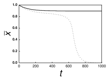
Figure 1: Behavior of the average fraction $\bar{x}$ of intact fibers with time $t$ (in units of the delay time) for the Gaussian distribution of $\bar{h}=1$ and $\sigma=0.2$. Solid and dotted lines correspond to $f=0.66$ and $0.68$, respectively.

Next the time evolution of the system is explored via direct numerical integration of the equation of motion (15). We consider realistic distributions of the threshold including the Gaussian distribution as well as the uniform one. Specifically, we set $\tau=100$ and use the time step $\Delta t=0.1$, mostly in a system of $N=10^{3}$ fibers. These parameter values have been varied, only to give no appreciable difference.

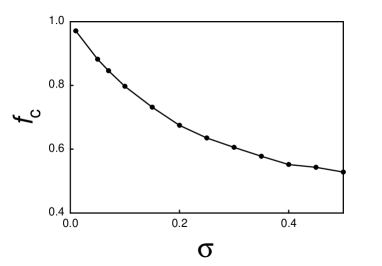
Figure 2: Critical stress $f_{c}$ versus variance $\sigma$

The typical behavior of the average fraction $\bar{x}$ of intact fibers is shown in Fig. 1 for the Gaussian distribution with unit mean $(\bar{h}=1)$ and variance $\sigma=0.2$. Note that for $f=0.66$ a large part of the fibers remain intact whereas all fibers become broken for $f=0.68$, indicating that the critical stress $f_{c}$ lies in between. Indeed this is the case in Fig. 2, which displays how the critical stress varies with the variance of the threshold distribution. It is of interest that after initial rupture $\bar{x}$ tends not to change much and exhibits a plateau as a function of time, which persists regardless of the details of the threshold distribution. This indicates that even for the stress strong enough to break all the fibers eventually, the system resists the stress for considerable time, followed by the complete rupture occurring suddenly. Note the sharp contrast with the results based on the conventional discrete-time recursive dynamics, where the strong stress brings about immediate failure bpc .

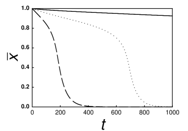
Figure 3: Behavior of the average fraction of intact fibers with time at $T=0.1$ for $f=0.48$ (solid line), $0.58$ (dotted line), and $0.68$ (dashed line). Other parameters are the same as those in Fig. 1.

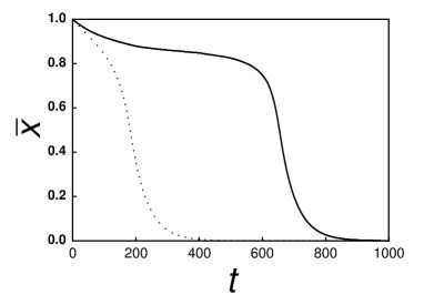
Figure 4: Comparison of the behavior at $T=0$ (solid line) and $0.1$ (dotted line). The stress is $f=0.68$ and other parameters are the same as those in Fig. 1.

We also examine the effects of noise ($T\neq 0$), which disallows the nontrivial solution in the stationary state and leads to $f_{c}=0$. Nevertheless Fig. 3 displays that the rupture time can be very long unless $f$ is not large. In a real system $T$ is nonzero but usually very small, and the complete rupture practically does not occur in the time scale of interest. For large $f$, the rupture is accelerated in the presence of noise, as shown in Fig. 4.

In summary, we have introduced realistic continuous-time dynamics for fiber bundles and investigated the behavior of the system under stress. The dynamics has been generalized to include uncertainty due to impurities and environmental influences. In its presence the system has been found always to break eventually, reflecting the irreversible nature of breaking, whereas in its absence all stationary features found in the deterministic recursion-equation approach have been reproduced. In particular disclosed is characteristic time evolution that the system tends to resist the stress for considerable time, followed by the complete rupture occurring suddenly. This has interesting implications to many systems in nature such as biological problems, the investigation of which is left for further study.

This work was supported in part by the Overhead Research Fund of SNU and in part by the Basic Research Program (Grant No. R01-2002-000-00285-0) of KOSEF.

References

- (1) See, e.g., R. da Silveira, Am. J. Phys. 67, 1177 (1999).
- (2) H.E. Daniels, Proc. R. Soc. London, Ser A 183, 405 (1945); F.T. Peirce, J. Text. Ind. 17, 355 (1926).
- (3) J.V. Anderson, D. Sornette, K.-t. Leung, Phys. Rev. Lett. 78, 2140 (1997).
- (4) D. Sornette, J. Phys. I 2, 2089 (1992).
- (5) S. Zapperi, P. Ray, H.E. Stanley, and A. Vespignani, Phys. Rev. Lett. 78, 1408 (1997).
- (6) B.D. Coleman, J. Appl. Phys. 29, 968 (1958); S.-d. Zhang, Phys. Rev. E 59, 1589 (1999); W.I. Newman and S.L. Phoenix, Phys. Rev. E 63 021507 (2001); L. Moral, Y. Moreno, J.B. Gomez, and A.F. Pacheco, Phys. Rev. E 63, 066106 (2001).
- (7) S.R. Pride and R. Toussaint, Physica A 312, 159 (2002).
- (8) F. Kun, R.C. Hidalgo, H.J. Hermann, and K. Pal, e-print cond-mat/0209308.
- (9) S. Roux, Phys. Rev. E 62, 6164 (2000); R. Scorretti, S. Ciliberto, and A. Guarino, Europhys. Lett. 55, 626 (2001).
- (10) A. Politi, S. Ciliberto, and R. Scorretti, e-print cond-mat/0206201; P. Bhattacharyya, S. Pradhan, and B.K. Chakrabarti, Phys. Rev. E 67, 046122 (2003); S. Pradhan and B.K. Chakrabarti, ibid. 67, 046124 (2003).
- (11) M.Y. Choi, Phys. Rev. Lett. 61, 2809 (1988); G.M. Shim, M.Y. Choi, and D. Kim, Phys. Rev. A 43, 1079 (1991).
- (12) Here is not directly related with the thermodynamic temperature of the system, considered in Refs. therm, and bpc, .
- (13) Then the problem corresponds to the Choi model of neural networks with . See Ref. myc, .