The violation of the Hund’s rule in semiconductor artificial atoms

Abstract

The unrestricted Pople-Nesbet approach for real atoms is adapted to quantum dots, the man-made artificial atoms, under applied magnetic field. Gaussian basis sets are used instead of the exact single-particle orbitals in the construction of the appropriated Slater determinants. Both system chemical potential and charging energy are calculated, as also the expected values for total and z-component in spin states. We have verified the validity of the energy shell structure as well as the Hund’s rule state population at zero magnetic field. Above given fields, we have observed a violation of the Hund’s rule by the suppression of triplets and quartets states at the $1p$ energy shell, taken as an example. We also compare our present results with those obtained using the $\mathbf{LS}$-coupling scheme for low electronic occupations. We have focused our attention to ground-state properties for GaAs quantum dots populated up to forty electrons.

The influence of spatial confinement on the physical properties such as the electronic spectra of

0D structures is a topic of growing interest. Among such systems one could select carriers and impurity atoms in metallic or semiconductor mesoscopic structures,jask as also atoms, ions and molecules trapped to microscopic cavities,jask ; conne ; riv ; waz ; beekman . In these systems, the confinement becomes important whenever a quantum sizes equal the cavity length. However, the energy spectrum of these systems is not only determined by the spatial confinement and its geometrical shape, but also by environmental facts such as electric and magnetic applied fields that break or lower the general symmetries. Finally, many-body effects as electron-electron interaction, may be even be more important than the confinement itself. In any case, a correct description of physical properties of the problem requires that the wavefunction must reflect both the form of confinement and the appropriated boundary conditions.

Interesting confined systems are the semiconductor quantum dots structures (QDs), also referred as man-made artificial atoms, built as low-dimensional electronic gases when crystalline translation invariance is broken in all three spatial dimensions and leading to discrete energy states, as in real atoms. Various are the approaches that have been used to deal with many-particle QDs. Among them, one can cite charging model,11 ; 12 ; 13 ; 14 correlated electron model,29 Green functions,30 Lanczos algorithm,16 Monte Carlo method,31 Hartree-Fock (HF) calculations,32 ; 33 ; 34 ; 35 and density functional theory.36

The charging model can reproduce well experimental findings for ”metallic dots”. On the opposite side, with much lower electronic density, the semiconductor dots requires a microscopic point of view to treat the electron-electron interaction.

Here we will consider a QD defined by a ”hard wall” spherical volume which is appropriated for semiconductors grown inside glass matrices. Some of the commonly studied topics are the formation of energy shells in their spectra,43 the control of their electronic correlations,44 the formation of Wigner molecules,45 and the influence of the Coulomb interaction in their spectra.46 ; 47 In these spherically defined artificial atoms both spin and orbital angular momenta are good quantum numbers, and the low occupation many-particle eigenstates can be labelled according to the $\mathbf{LS}$-coupling scheme,condon . For occupation number above four, the $\mathbf{LS}$-coupling scheme becomes extremely cumbersome and, in this paper, we have chosen the unrestricted Pople-Nesbet matrix approachszabo of the single determinant self-consistent HF formalism to treat shell configurations of dots containing up to forty electrons, where we have calculated the total spin expected values, chemical potential and charging energy. We show the changes induced by the magnetic field on such approach, using a set of Gaussian basis (section II). Then we discuss our main results (section III) by focusing on how magnetic field determines the Zeeman splitting and induces violation of the Hund’s rule.

Within the Unrestricted Hartree-Fock formalism (UHF), the $\alpha$ (spin-up) and $\beta$ (spin-down) functions have different spatial components, $\chi_{i}(\mathbf{x})=\left\{\psi_{j}^{\alpha}(\mathbf{r})\alpha(\omega),\psi_{j}^{\beta}(\mathbf{r})\beta(\omega)\right\}$, described by the orbitals $\left\{\psi_{j}^{\alpha}|j=1...k\right\}$ ($\{\psi_{j}^{\beta}|j=1...k\}$). Therefore, an UHF wavefunction has the form $\left|\Psi^{UHF}\right\rangle=\left|\psi_{1}^{\alpha}\overline{\psi}_{1}^{\beta}...\right\rangle$, which represents open shells once no spatial orbital can be doubly occupied. The closed shells can be also obtained,szabo more specifically, UHF functions are not necessarily system eigenstates having well defined $L$ and $S$ values. Yet, the number of carrier, $N$, must equal the the sum of spin-up and spin-down electrons, as $N=N^{\alpha}+N^{\beta}$. The integration of the spin degrees of freedomszabo yields two coupled HF equations that must be simultaneously solved. They have the form $f^{\alpha/\beta}\left|\psi_{j}^{\alpha/\beta}\right\rangle=\varepsilon_{j}^{\alpha/\beta}\left|\psi_{j}^{\alpha/\beta}\right\rangle$, where the respective Fock operators are given by

$$f^{\alpha/\beta}=h_{j}+\sum_{a}^{N^{\alpha/\beta}}\left[J_{a}^{\alpha/\beta}-K_{a}^{\alpha/\beta}\right]+\sum_{a}^{N^{\beta/\alpha}}J_{a}^{\beta/\alpha}\text{.}$$ (1)

Both $f^{\alpha}$ and $f^{\beta}$ include the kinetic($h_{j}$), the direct( $J_{a}^{\alpha/\beta}$) and the exchange ($K_{a}^{\alpha/\beta}$) terms between electrons with same spin, and a direct term ($J_{a}^{\beta/\alpha}$ ) between electrons with opposite spins. The interdependence among $f^{\alpha}$ ($f^{\beta}$) and $\psi_{j}^{\beta}$ ($\psi_{j}^{\alpha}$) requires the simultaneous solution of the two HF equations. They yield the sets $\left\{\psi_{j}^{\alpha}\right\}$ and $\left\{\psi_{j}^{\beta}\right\}$ that should minimize the energy $E_{0}^{UHF}$ of the unrestricted ground-state, $\left|\Psi_{0}^{UHF}\right\rangle$, given by

$$E_{0}^{UHF} = \sum_{a}^{N^{\alpha}}h_{aa}^{\alpha}+\sum_{a}^{N^{\beta}}h_{aa}^{\beta}+\frac{1}{2}\sum_{a}^{N^{\alpha}}\sum_{b}^{N^{\alpha}}\left[J_{ab}^{\alpha\alpha}-K_{ab}^{\alpha\alpha}\right]$$ (2)

$$+\frac{1}{2}\sum_{a}^{N^{\beta}}\sum_{b}^{N^{\beta}}\left[J_{ab}^{\beta\beta}-K_{ab}^{\beta\beta}\right]+\sum_{a}^{N^{\alpha}}\sum_{b}^{N^{\beta}}J_{ab}^{\alpha\beta}\text{.}$$

In these expressions, $h_{aa}^{\alpha/\beta}=\left\langle\psi_{a}^{\alpha/\beta}\right|h_{a}\left|\psi_{a}^{\alpha/\beta}\right\rangle$, $J_{ab}^{\alpha\beta}=\left\langle\psi_{a}^{\alpha}\right|J_{b}^{\beta}\left|\psi_{a}^{\alpha}\right\rangle=\left\langle\psi_{b}^{\beta}\right|J_{a}^{\alpha}\left|\psi_{b}^{\beta}\right\rangle=J_{ba}^{\beta\alpha}$, $J_{ab}^{\alpha\alpha}=\left\langle\psi_{a}^{\alpha}\right|J_{b}^{\alpha}\left|\psi_{a}^{\alpha}\right\rangle=\left\langle\psi_{b}^{\alpha}\right|J_{a}^{\alpha}\left|\psi_{b}^{\alpha}\right\rangle=J_{ba}^{\alpha\alpha}$ (with an analog term for $J_{ab}^{\beta\beta}$), and $K_{ab}^{\alpha\alpha}=\left\langle\psi_{a}^{\alpha}\right|K_{b}^{\alpha}\left|\psi_{a}^{\alpha}\right\rangle=\left\langle\psi_{b}^{\alpha}\right|K_{a}^{\alpha}\left|\psi_{b}^{\alpha}\right\rangle=K_{ba}^{\alpha\alpha}$ (with an analog term for $K_{ab}^{\beta\beta}$).

The Pople-Nesbet approach transforms the UHF equations into a matrix formulation by expanding $\psi_{i}^{\alpha/\beta}$ in a set of known basis functions $\left\{\phi_{\nu}|\nu=1...k\right\}$,

$$\psi_{i}^{\alpha/\beta}=\sum_{\nu}C_{\nu i}^{\alpha/\beta}\phi_{\nu}\text{,}$$ (3)

where the expansion coefficients $C_{\nu i}^{\alpha/\beta}$ become the parameters to be iterated. When Eq. 3 is inserted into Eq. 1 one obtains the $k$ $\times$ $k$ coupled matrix equations,

$$\mathbf{F}^{\alpha/\beta}\mathbf{C}^{\alpha/\beta}=\mathbf{SC}^{\alpha/\beta}\mathbf{\varepsilon}^{\alpha/\beta}\text{,}$$ (4)

where $\mathbf{S}$ is the positive defined overlap ($S_{\mu\nu}=\left\langle\phi_{\mu}\right.\left|\phi_{\nu}\right\rangle$) between basis functions, $\mathbf{C}^{\alpha/\beta}$ are the expansion coefficient matrices whose columns describe each spatial orbital $\psi_{i}^{\alpha/\beta}$, $\mathbf{\varepsilon}^{\alpha/\beta}$ are the diagonal matrices of the orbital energies ($\varepsilon_{i}^{\alpha/\beta}$), and $\mathbf{F}^{\alpha/\beta}$ are the Fock operators,

$$F_{\mu\nu}^{\alpha/\beta}=\int d^{3}\mathbf{r}\phi_{\mu}^{\ast}(\mathbf{r})f^{\alpha/\beta}\phi_{\nu}(\mathbf{r})\text{.}$$ (5)

At this point becomes convenient to introduce the charge density for the spin-up and -down electrons, defined as $\rho^{\alpha/\beta}(\mathbf{r})=\sum_{a}^{N^{\alpha/\beta}}\left|\psi_{a}^{\alpha/\beta}(\mathbf{r})\right|^{2}=\sum_{\mu}\sum_{\nu}P_{\mu\nu}^{\alpha/\beta}\phi_{\mu}(\mathbf{r})\phi_{\nu}^{\ast}(\mathbf{r})$, where the elements of the respective density matrices are $P_{\mu\nu}^{\alpha/\beta}=\sum_{a}^{N^{\alpha/\beta}}C_{\mu a}^{\alpha/\beta}C_{\nu a}^{\alpha/\beta\ast}$. Thus, one can define two new quantities: i) The total charge density, $\rho^{T}(\mathbf{r})=\rho^{\alpha}(\mathbf{r})+\rho^{\beta}(\mathbf{r})$, that determines $N$ when integrated over all space; ii) The spin density, $\rho^{S}(\mathbf{r})=\rho^{\alpha}(\mathbf{r})-\rho^{\beta}(\mathbf{r})$, that yields $2M_{S}$ after integration over all space. The unrestricted wavefunctions are eigenfunctions of $S_{Z}$, but not necessarily of $S^{2}$, therefore one can define the total charge ( $\mathbf{P}^{T}=\mathbf{P}^{\alpha}+\mathbf{P}^{\beta}$) and the spin ( $\mathbf{P}^{S}=\mathbf{P}^{\alpha}-\mathbf{P}^{\beta}$) density matrices for the system. The elements of the two Fock matrices are obtained as $F_{\mu\nu}^{\alpha/\beta}=T_{\mu\nu}+G_{\mu\nu}^{\alpha/\beta}$, where $T_{\mu\nu}=-\hbar^{2}/(2m)\left\langle\phi_{\mu}\right|\nabla^{2}\left|\phi_{\nu}\right\rangle$ and $G_{\mu\nu}^{\alpha/\beta}=e^{2}/\varepsilon\sum_{\lambda}\sum_{\sigma}[P_{\lambda\sigma}^{T}\left\langle\phi_{\mu}\phi_{\sigma}\right|\left|\mathbf{r}_{1}-\mathbf{r}_{2}\right|^{-1}\left|\phi_{\nu}\phi_{\lambda}\right\rangle-P_{\lambda\sigma}^{\alpha/\beta}\left\langle\phi_{\mu}\phi_{\sigma}\right|\left|\mathbf{r}_{1}-\mathbf{r}_{2}\right|^{-1}\left|\phi_{\lambda}\phi_{\nu}\right\rangle]$, with $\varepsilon$ being the material dielectric constant.

The self-consistency lies in the fact that both $\mathbf{F}$ and $\mathbf{P}$ depend on $\mathbf{C}$, while the coupling of spin-up and -down equations occurs since $\mathbf{F}^{\alpha}$ ($\mathbf{F}^{\beta}$) depends on $\mathbf{P}^{\beta}$ ($\mathbf{P}^{\alpha}$) through $\mathbf{P}^{T}$.

The procedure to solve Eq. 4 is: i) Given a confinement potential, one specifies $N$ and $\left\{\phi_{\mu}\right\}$; ii) The integrations on $S_{\mu\nu}$ and $T_{\mu\nu}$ are performed; iii) An initial guess is used for $\mathbf{P}^{\alpha/\beta}$ and $\mathbf{P}^{T}$, perform two-electron integrals for $\mathbf{G}^{\alpha/\beta}$ and $\mathbf{T}$ to construct $\mathbf{F}^{\alpha/\beta}$.    Diagonalize $\mathbf{F}^{\alpha/\beta}$ to get $\mathbf{C}^{\alpha/\beta}$ and $\mathbf{\varepsilon}^{\alpha/\beta}$, and form new $\mathbf{P}^{\alpha/\beta}$; iv) This iteration is repeated until the desired convergence for $E_{0}^{UHF}$ is reached. The Pople-Nesbet ground-state energy is

$$E_{0}^{UHF}=\frac{1}{2}\sum_{\mu}\sum_{\nu}\left[P_{\nu\mu}^{T}T_{\mu\nu}+P_{\nu\mu}^{\alpha}F_{\mu\nu}^{\alpha}+P_{\nu\mu}^{\beta}F_{\mu\nu}^{\beta}\right]\text{ .}$$ (6)

The unrestricted functions are not, in general, eigenstates of $S^{2}$, thus we calculate the spin expectation values as szabo

$$\left\langle S^{2}\right\rangle_{UHF} = \left(\frac{N^{\alpha}-N^{\beta}}{2}\right)\left(\frac{N^{\alpha}-N^{\beta}}{2}+1\right)+N^{\beta}$$ (7)

$$-\sum_{a}^{N^{\alpha}}\sum_{b}^{N^{\beta}}\left[\sum_{\mu}\sum_{\nu}C_{\mu a}^{\alpha\text{ }\ast}C_{\nu b}^{\beta}S_{\mu\nu}\right]^{2}\text{,}$$

and

$$\left\langle S_{Z}\right\rangle_{UHF}=\frac{1}{2}\sum_{\mu}\sum_{\nu}\left(P_{\nu\mu}^{\alpha}-P_{\nu\mu}^{\beta}\right)S_{\mu\nu}\text{.}$$ (8)

As an application of the Pople-Nesbet approach, we consider a QD with radius $R_{0}$ confined to an infinite spherical potential in the presence of a magnetic field $\mathbf{B}=(0,0,B_{0})$ and populated up to forty electrons. Its single-particle Hamiltonian is

$$H_{0}=\frac{\hbar^{2}}{2m}\left(\mathbf{k}+\frac{e}{\hbar c}\mathbf{A}\right)^{2}+g\frac{\mu_{B}}{\hbar}\mathbf{B}\cdot\mathbf{S}\text{,}$$ (9)

where $\mu_{B}$ is the Bohr magneton, $g$ is the bulk $g$-factor, and we use the symmetric gauge, $\mathbf{A}=(\mathbf{B}\times\mathbf{r})/2$. Using atomic units, $E_{Ry}=e^{2}/(2a_{0})$(Rydberg) for the energy, and $a_{0}=\hbar^{2}/(m_{0}e^{2})$(Bohr radius) for length, the Hamiltonian $H_{0}$ can be written in dimensionless form

$$H_{0} = \frac{1}{\widetilde{m}}\frac{a_{0}^{2}}{R_{0}^{2}}\left[-\frac{1}{x^{2}}\frac{\partial}{\partial x}\left(x^{2}\frac{\partial}{\partial x}\right)+\frac{\mathbf{L}^{2}}{x^{2}}\right.$$

$$\left.+\frac{R_{0}^{2}}{2l_{B}^{2}}\left(L_{Z}+\widetilde{m}gS_{Z}\right)+\frac{R_{0}^{4}}{4l_{B}^{4}}x^{2}\sin^{2}(\theta)\right]\text{,}$$

where $\widetilde{m}=m/m_{0}$, $l_{B}=\sqrt{\hbar c/(eB_{0})}$ is the magnetic length, and $x=r/R_{0}$. Without magnetic field, the normalized spatial eigenfunctions of $H_{0}$ are given by

$$\phi_{\nu}(\mathbf{r})=\left[\frac{2}{R_{0}^{3}}\frac{1}{\left[j_{l+1}\left(\alpha_{nl}\right)\right]^{2}}\right]^{1/2}j_{l}\left(\alpha_{nl}x\right)Y_{l,m_{l}}(\theta,\phi)\text{.}$$ (11)

The boundary condition at the surface, $r=R_{0}$ (or $x=1$), determines $\alpha_{nl}$ as the $n^{th}$ zero of the spherical Bessel function $j_{l}(\alpha_{nl}x)$ and $Y_{l,m_{l}}(\theta,\phi)$ is the spherical harmonic.

The Hamiltonian for the electron-electron interaction in atomic units becomes $H_{ee}=(a_{0}/R_{0})2/(\varepsilon\left|\mathbf{x}_{1}-\mathbf{x}_{2}\right|)$, where the usual multipole expansion for $|\mathbf{x}_{1}-\mathbf{x}_{2}|^{-1}$ is used in our calculations.

The spatial orbitals in $\psi_{i}^{\alpha/\beta}$ define the six lowest energy shells ($1s$, $1p$, $1d$, $2s$, $1f$, $2p$) without magnetic field,walecka . Thus, the index $\nu\equiv n,l,m_{l}$ can assume up to $40$ ($20$ spin-up and $20$ -down) possible values for those shells. Certainly, the magnetic field lifts both spin and orbital degeneracies. Let us consider a GaAs dot, a wide-gap semiconductor having $\widetilde{m}=0.065$, $g=0.45$ and $\varepsilon=12.65$.

The inclusion of a magnetic field requires modifications on the UHF equations. The spin-independent linear and quadratic magnetic terms are easyly added to the definitions of both $h$ in $f^{\alpha/\beta}$ and $T_{\mu\nu}$. However, the inclusion of the spin-dependent linear term ($\sim B_{0}S_{Z}$) to $h$ in $f^{\alpha/\beta}$ requires decomposition of kinetic and Coulomb terms into $T_{\mu\nu}^{\alpha/\beta}$ and $G_{\mu\nu}^{\alpha/\beta}$. Thus, under a magnetic field we should make the substitution $P_{\nu\mu}^{T}T_{\mu\nu}\Rightarrow P_{\nu\mu}^{\alpha}T_{\mu\nu}^{\alpha}+P_{\nu\mu}^{\beta}T_{\mu\nu}^{\beta}$ in $E_{0}^{UHF}$ (Eq. 6).

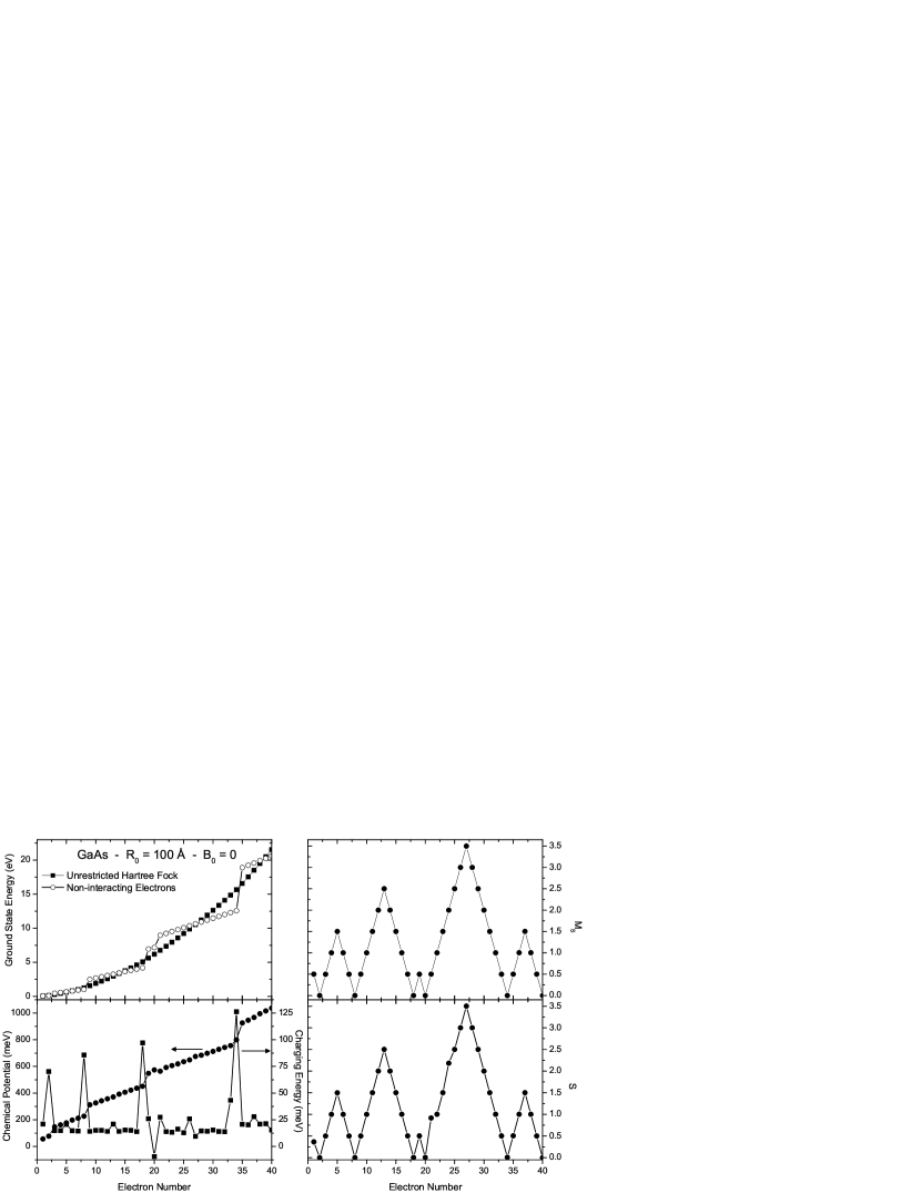
Figure 1: Unrestricted ground-state energy for a $R_{0}=100$ Å GaAs QD without magnetic field. In the upper left panel we compare the unrestricted and the non-interacting energies, where the QD energy shell structure is visible. The bottom left panel shows QD chemical potential (left scale) and charging energy (right scale). The former displays abrupt change always when a new shell starts to be populated, while the latter presents larger (smaller) peaks when a shell is fully filled (half-filled), a direct consequence of the Hund’s rule. The bottom and upper right panels show, respectively, the $N$-evolution of the expected values of total spin and its z-projection.

Another important detail refers to the orbital basis $\left\{\phi_{\nu}|\nu=1...k\right\}$. Instead of the exact spherical Bessel functions of Eq.11, the radial part of each orbital was decomposed in a sum involving five Gaussians confined to region $x\leq 1$, while the angular part is maintained as defined by its symmetry, as

$$\phi_{n,l,m_{l}}(x,\theta,\phi) = N_{nl}\left(1-x\right)^{n}x^{l}\prod_{i=1}^{n-1}\left(\widetilde{\alpha}_{il}-x\right)$$

$$\times\sum_{k=1}^{5}V_{k}e^{-D_{k}R_{0}^{2}x^{2}}Y_{l,m_{l}}(\theta,\phi)\text{,}$$

where $N_{nl}$ is the normalization, the polynomial $\left(1-x\right)^{n}$ garanties the boundary $x=1$, the polynomial in $x^{l}$ is required for $l>0$ states at the origin $x=0$, the product in $\left(\widetilde{\alpha}_{il}-x\right)$ nulls functions at the zeros $\widetilde{\alpha}_{il}$ of the respective spherical Bessel function transposed to the interval $0\leq x\leq 1$, and the last sum involves an expansion into $5$ Gaussians. Higher order expansion did not show any improvement for $N\leq 40$. The Gaussian coefficients $V_{k}$ and exponents $D_{k}$ are determined for each value of $R_{0}$, by maximizing the superposition between Eqs. 11 and The violation of the Hund’s rule in semiconductor artificial atoms. Once $V_{k}$ and $D_{k}$ are determined, we run our UHF code for each value of $R_{0}$ and $N$ , and find the parameters $C_{\nu i}^{\alpha/\beta}$ that better describe Eq. 3 and give the minimal energy in Eq. 6.

At last, we have calculated two quantities that will be used in the description of our results. The first one is the QD chemical potential, which yields the energy difference between two successive ground states,

$$\mu_{dot}(N)=E_{0}(N)-E_{0}(N-1)\text{ .}$$ (13)

The second one is the QD charging energy, which yields the energy cost to add an extra electron to the system,

$$E_{char}(N)=E_{0}(N+1)-2E_{0}(N)+E_{0}(N-1)\text{ .}$$ (14)

From these two last equations, one can also see that $E_{char}(N)=\mu_{dot}(N+1)-\mu_{dot}(N)$.

We show in Fig. 1 the results of a UHF Pople-Nesbet calculation for a GaAs QD having $R_{0}=100$ Å, at zero magnetic field. In the left upper panel we have compared the non-interacting electron problem and the UHF results as function of occupation. The shell structure occurs for magic numbers $N=2$, $8$, $18$, $20$, $34$ and $40$. It is observed that electron-electron interaction decreases (increases) the non-interacting ground-state energy when occupation corresponds to a shell less (more) than half-filled. At exactly half-filled cases $N=5$, $13$, $27$ and $37$, the interacting and non-interacting energy values are approximately equal.

In the bottom left panel of Fig. 1 we show both QD chemical potential (left scale, Eq. 13) and charging energy (right scale, Eq. 14), where the respective values of $E_{0}$ were obtained from the unrestricted calculation presented in the left upper panel. Notice that $\mu_{dot}$ linearly increases as the occupation increases inside a given shell. When such shell is totally filled, there is an abrupt change in $\mu_{dot}$ indicating that the following shell starts its occupation. Also, the higher the occupation, the more abrupt is this change. An anomalous behavior seems to occur with the $2s$ shell, whose $\mu_{dot}$-value is larger than the $1f$ shell, that has higher energy. The charging energy is another form to verify not only the presence of shell strusture in the spectrum, but also the validity of Hund’s rule for the filling of such shells. In principle, $E_{char}$ must present larger (smaller) peaks when the total (half) occupation of a shell is achieved. The first fact is due to the higher difficulty in adding an electron to a QD in a filled shell state, while the second one refers to Hund’s rule, which states that electrons must be added to the system with their spin being parallel, until all possible orbitals inside a given shell be occupied, making the total energy of the system be decreased because of the maximized exchange contribution. However, some discrepancies are verified in $E_{char}$: the smaller peak of $N=27$ occurs here at $N=26$, and the larger peak of $N=20$ is negative.

Figure 2: Violation of Hund’s rule induced by magnetic field in the $R_{0}=100$ Å GaAs QD of the previous figure. The panels show the successive occupation (indicated in the upper right corner of each panel) of the $1p$ shell, assuming that the $1s$ shell remains populated by one spin-up and one spin-down electron. The possible spin configurations for given $N$ are indicated by $+$ (spin-up) and $-$ (spin-down). For $B_{0}=0$ the spin sequence is $1/2-1-3/2-1-1/2-0$, while at fields higher than $3$ T, it changes to $1/2-0-1/2-0-1/2-0$. It interesting to observe that a magnetic field can suppress the energy triplets and quartets from the QD spectrum.

The right bottom and upper panels of Fig.1 show respectively the $N$-evolution of the total spin $S$ and its projection $M_{S}$ as calculated from Eqs. 7 and 8 for the unrestricted energies. Notice that, with no magnetic field, Hund’s rule seems to be followed; the $M_{S}$ expected value oscillates from $0$ in a filled shell to its maximum in a half-filled shell, when it starts to decrease again on the way to the closing of the shell; the maxima are $M_{S}=1/2$, $3/2$, $5/2$ and $7/2$ for $s$, $p$, $d$ and $f$ shells, respectively. The $S$ expected value yielded by the unrestricted formalism is also very reasonable; discrepancies are only observed at $N=24$, where $S>2$, and at $N=21$, where $S>1/2$. We believe that both discrepancies related to the $2s$ shell or to its surroundings - $\mu_{dot}$ larger than the one of $1f$ shell, negative peak for $N=20$ in $E_{char}$, and almost doubled $S$ expected value for $N=21$ - are caused by the non-reasonable Gaussian reproduction of this orbital.artigo

By focusing on the $1p$ shell we show in Fig. 2, for the same QD of the previous figure, how a finite magnetic field is able to violate Hund’s rule in the system. Panels from left to right and from up to bottom show the successive ground state energies from $N=3$ to $N=8$ as this shell is filled, always considering that the $1s$ shell remain fully occupied by two electrons, one up and one down; the distinct possible spin configurations for each $N$ are indicated by $+$ (up) and $-$ (down). In addition to the small Zeeman effect present in all occupations, there is a changing of ground state spins at $N=4$, $5$ and $6$ as the field is increased. Notice that at zero field the spin sequence is $1/2-1-3/2-1-1/2-0$; in a field above $3$ T it becomes $1/2-0-1/2-0-1/2-0$, meaning that quartets and triplets are suppressed by the magnetic field, and the ground state of the system starts to oscillate only between singlets and doublets at high fields as $N$ increases. When this $1p$ shell is half-filled ($N=5$), the ground state goes from a quartet to a doublet at $B_{0}\simeq 2$ T; when it has one electron more ($N=6$) or less ($N=4$) than that, it goes from a triplet to a singlet at $B_{0}\simeq 3$ T.

At last, in order to prove the efficiency of the Pople-Nesbet approach, we compared the results from this UHF self-consistent matrix formulation with the ones obtained from the $\mathbf{LS}$-coupling scheme used in Ref. [LS, ], where a GaAs QD having $R_{0}=90$ Å was considered, and the quadratic term in $B_{0}$ was neglected since only small fields were considered; also, only $N=2$ and $N=3$ occupations were calculated, since the states were exactly built (not only a single Slater determinant), and the electron-electron interaction was included by using perturbation theory, justified at such radius. At zero field the energies for $N=2$ are $16.5$ meV ($\mathbf{LS}$) and $16.1$ meV (UHF), while for $N=3$ they are $34.8$ meV ($\mathbf{LS}$) and $33.9$ meV (UHF); so, the formalism here used indeed give smaller ground state energies than the $\mathbf{LS}$ perturbation scheme. We have also checked the validity of neglecting the quadratic term in $B_{0}$ for fields smaller than $2$ T. One should emphasize that a disadvantage of the UHF approach is that, in principle, it is not sure that one gets trustable information about the $L$ and $S$ expected values of QD states; on the other hand, the applicability of the $\mathbf{LS}$ scheme is highly decreased as the QD occupation increases.

We have shown how the unrestricted Pople-Nesbet approach applied to a spherical QD under a magnetic field yields a reasonable description of its energetic spectrum, where a maximum occupation of $40$ electrons has been considered. We have seen how both QD chemical potential and charging energy reproduce the filling and half-filling structures of its energy shells at zero field. With the total spin expected value for each occupation in a given radius, we have seen that the Hund rule is satisfied at zero field; however, under a finite field, we have shown that it is violated and, at given values of the field which depend on QD parameters, transitions that change a given ground state symmetry are observed.

We acknowledge support from FAPESP-Brazil.

References

- (1) W. Jaskólski, Phys. Rep. 271, 1 (1996).
- (2) J. P. Connerade, V. K. Dolmatov, P. A. Lakshmit, J. Phys. B: At. Mol. Opt. Phys. 33, 251 (2000).
- (3) R. Rivelino, J. D. M. Vianna, J. Phys. B: At. Mol. Opt. Phys. 34, L645 (2001).
- (4) D. Bielinska-Waz, J. Karkowski, G. H. F. Diercksen, J. Phys. B: At. Mol. Opt. Phys. 34, 1987 (2001).
- (5) R. A. Beekman, M. R. Roussel, P. J. Wilson, Phys. Rev. A 59, 503 (1999).
- (6) D. V. Averin, A. N. Korothov, K. K. Likharev, Phys. Rev. B 44, 6199 (1991).
- (7) C. W. J. Beenakker, Phys. Rev. B 44, 1646 (1991).
- (8) H. Grabert, Z. Phys. B 85, 319 (1991).
- (9) L. P. Kouwenhoven, N. C. van der Vaart, A. T. Johnson, W. Kool, C. J. P. M. Harmans, J. G. Williamson, A. A. M. Staring, C. T. Foxon, Z. Phys. B 85, 367 (1991).
- (10) D. Weinmann, W. Häusler, B. Kramer, Ann. Phys. 5, 652 (1996).
- (11) G. Cipriani, M. Rosa-Clot, S. Taddei, Phys. Rev. B 61, 7536 (2000).
- (12) K. Jauregui, W. Häusler, D. Weinmann, B. Kramer, Phys. Rev. B 53, R1713 (1996).
- (13) J. Harting, O. Mülken, P. Borrmann, Phys. Rev. B 62, 10207 (2000).
- (14) D. Pfannkuche, V. Gudmundsson, P. A. Maksym, Phys. Rev. B 47, 2244 (1993).
- (15) Y. Alhassid, S. Malhotra, Phys. Rev. B 66, 245313 (2002).
- (16) B. Reusch, H. Grabert, Phys. Rev. B 68, 045309 (2003).
- (17) S. Bednarek, B. Szafran, J. Adamowski, Phys. Rev. B 59, 13036 (1999).
- (18) M. Ferconi, G. Vignale, Phys. Rev. B 50, 14722 (1994).
- (19) W. D. Heiss, R. G. Nazmitdinov, Phys. Rev. B 55, 16310 (1997).
- (20) Y. E. Lozovik, S. Y. Volkov, Phys. Sol. Stat. 45, 364 (2003).
- (21) P. A. Sundqvist, S. Y. Volkov, Y. E. Lozovik, M. Willander, Phys. Rev. B 66, 075335 (2002).
- (22) R. K. Pandey, M. K. Harbola, V. A. Singh, Phys. Rev. B 67, 075315 (2003).
- (23) B. Szafran, J. Adamowski, S. Bednarek, Physica E 4, 1 (1999).
- (24) E. U. Condon and G. H. Shortley, The Theory of Atomic Spectra (Cambridge University Press, London, 1977).
- (25) A. Szabo, N. S. Ostlund, Modern Quantum Chemistry: Introduction to Advanced Electronic Structure Theory (Dover, New York, 1999).
- (26) A. L. Fetter, J. D. Walecka, Quantum Theory of Many-Particle Systems (McGraw-Hill, San Francisco, 1971).
- (27) C. F. Destefani, J. D. M. Vianna, G. E. Marques, submitted to J. Phys. B: At. Mol. Opt. Phys. (physics/0404007).
- (28) C. F. Destefani, G. E. Marques, and C. Trallero-Giner, Phys. Rev. B 65, 235314 (2002).