Nonequilibrium transfer and decoherence in quantum impurity problems

Abstract

Using detailed balance and scaling properties of integrals that appear in the Coulomb gas reformulation of quantum impurity problems, we establish exact relations between the nonequilibrium transfer rates of the boundary sine-Gordon and the anisotropic Kondo model at zero temperature. Combining these results with findings from the thermodynamic Bethe ansatz, we derive exact closed form expressions for the transfer rate in the biased spin-boson model in the scaling limit. They illustrate how the crossover from weak to strong tunneling takes place. Using a conjectured correspondence between the transfer and the decoherence rate, we also determine the exact lower bound for damping of the coherent oscillation as a function of bias and dissipation strength in this paradigmic model for NMR and superposition of macroscopically distinct states (qubits).

I Introduction

Quantum impurity problems (QIPs) have attracted a great deal of interest recently. This is because the underlying physics is non-trivial and the models are manageable technically despite their essentially nonperturbative nature. In addition, they have a multitude of experimental applications, including the Kondo effect, quantum dots, dissipative quantum mechanics, tunneling in quantum wires and fractional quantum Hall devices.weissbook

There have been discovered various relations between thermodynamic quantities of the anisotropic Kondo model (AKM) and the boundary sine-Gordon (BSG) field theory model.fendley95a Each of these integrable models is of considerable interest and it is remarkable that they are closely related. They are both boundary integrable quantum field theories with a quantum-group spin at the boundary which takes values in standard or cyclic representations of the quantum group $SU(2)_{q}$.fendley95c

The AKM is related to the spin-boson (SB) model. leggett87 The BSG model is equivalent to the Schmid model, which describes a damped particle in a tilted cosine potential schmid83 and has a great variety of applications to charge and particle transport including Josephson junction dynamics. weissbook The field theory limit in the AKM and BSG model corresponds to the Ohmic scaling limit in the SB and Schmid model. Here we are interested in the strong-backscattering or tight-binding (TB) representations of these models. The equivalence and difference of the various models can most easily be seen in the Anderson-Yuval Coulomb gas representation for the partition function, which is the grandcanonical sum of a one-dimensional classical gas of positive and negative unit charges with ”log-sine” interactions and overall neutrality. The AKM or SB model differs from the BSG or Schmid model by a different charge ordering. Principally in the sequel, we concentrate on the Schmid and SB model and use the language of dissipative quantum mechanics. With use of the correspondence relations, our results directly apply also to the BSG and the anistropic Kondo model.

Here we study nonequilibrium quantum dynamics of the models mentioned with the rigorous Keldysh approach. Upon uncovering functional relations between perturbative Coulomb integrals, we discover that at zero temperature for every particular transfer rate only paths with minimal number of tunneling moves contribute. This allows us then to find the characteristic function encapsulating all statistical fluctuations of the transport process. The results for the Schmid model corroborate the findings from the thermodynamic Bethe ansatz. We discover, as a second result of current interest, an intriguing functional relation between transfer rates in the Schmid and partial transfer rates in the SB model. The major result is given in Eq. (73). Using this, we derive a concise contour integral expression for the transfer rate in the SB model [cf. Eq. (86)], from where we find both the weak- and the strong-tunneling expansion for this rate. We also make and check a conjecture which relates the transfer rate to the decoherence rate in the SB model. The ensuing asymptotic series, Eq. (100), provides an exact lower bound for decoherence in the scaling limit as a function of bias and damping strength.

In the following section, we briefly review a general Poissonian transport model with transfer rates describing direct forward and backward transitions by $m$ states, $m=1,\,2,\,3,\cdots$. We solve the master equation and determine the evolution of the probability distribution. In Sec. III, we study the Schmid model in the real-time Coulomb gas representation, which is based on the nonequilibrium Keldysh method. Upon performing a cluster decomposition, we show that the BSG dynamics at long times represents a realization of the Poissonian dynamics studied in Sec. II. We derive exact formal expressions for the quantum transfer rates in which friction and noise effects are clearly separated. The corresponding investigation for the AKM or SB model is presented in Sec. IV. The weak-tunneling expansion for the transfer rates at zero temperature are studied both for the Schmid and SB model in Sec. V. Using detailed balance relations, and scaling properties holding for a subgroup of the Coulomb integrals, we uncover a multitude of linear functional relations between the occuring Coulomb integrals of same order. Using these relations, we discover formidable cancellations in the path sum for the individual rates of the Schmid model such that only the paths with minimal number of tunneling moves contribute. This peculiarity allows us to determine all statistical fluctuations once the current is known. The corresponding discussion is given in Subsec. V.5. We also discover an intriguing functional relation between the rates in the Schmid model and the partial rates in the SB model. The findings in Sec. V can be used to shed light on the entire regime from weak to strong tunneling, both in the Schmid and SB model. In Sec. VI, we derive from the perturbative series an exact integral representation for the transfer rate in the SB model at zero temperature valid for general coupling, bias and damping strengths. From that, the asymptotic (strong-tunneling) expansion for the transfer rate is derived. In Subsec. VI.3, we propose a conjecture about a simple close relation between the relaxation and decoherence rate in the SB model. The conjectured formula for the decoherence rate is in agreement with all known special cases and gives a lower bound on decoherence for general bias and damping strength. Finally, in Subsec. VI.4 we give analytic expressions for the leading thermal corrections.

II Poissonian transport and noise

Consider a general model describing transport of mass or charge between sites $n=0,\,\pm 1,\,\pm 2,\cdots$ via direct forward and backward transitions by $\ell$ sites, $\ell=1,\,2,\cdots$. The respective weights per unit time (transfer “rates”) are denoted by $\gamma_{\ell}^{\pm}$. Assuming statistically independent transitions, the dynamics of the population probability $P_{n}(t)$ of site $n$ is governed by the master equation

$$\dot{P}_{n}(t)=\!\sum_{\ell=1}^{\infty}\left[\gamma_{\ell}^{+}P_{n-\ell}(t)+\gamma_{\ell}^{-}P_{n+\ell}(t)-(\gamma_{\ell}^{+}\!+\!\gamma_{\ell}^{-})P_{n}(t)\right]\,.$$

The Fourier transform $\tilde{P}(k,t)=\sum_{n}e^{ikn}\,P_{n}(t)$ with initial state $P_{n}(0)=\delta_{n,0}$ is found from this equation as

$$\tilde{P}(k,t)=\prod_{n=1}^{\infty}\exp\left[t\left(e^{ikn}-1\right)\gamma_{n}^{+}+t\left(e^{-ikn}-1\right)\gamma_{n}^{-}\right].$$

The moments of the probability distribution follow from the characteristic function $\tilde{P}(k,t)$ by differentiation,

$$\left<n^{m}(t)\right>\equiv\sum_{n}n^{m}P_{n}(t)=\left.\left(-i\frac{\partial}{\partial k}\right)^{m}\tilde{P}(k,t)\right|_{k=0}\;.$$ (1)

The resulting expressions can be written in terms of the irreducible moments or cumulants $\left<n^{m}(t)\right>_{c}$ as

$$\left<n(t)\right> = \left<n(t)\right>_{c}\;,$$

$$\left<n^{2}(t)\right> = \left<n(t)\right>_{c}^{2}+\left<n^{2}(t)\right>_{c}\;,$$ (2)

$$\left<n^{3}(t)\right> = \left<n(t)\right>_{c}^{3}+3\left<n^{2}(t)\right>_{c}\left<n(t)\right>_{c}+\left<n^{3}(t)\right>_{c}\;.$$

The cumulants expansion

$$\ln\tilde{P}(k,t)=\sum_{m=1}^{\infty}\frac{(ik)^{m}}{m!}\left<n^{m}(t)\right>_{c}$$ (3)

leads us to the expressions

$$\begin{array}[]{rcl}\left<n^{m}(t)\right>_{c}&=&{\displaystyle\left.\left(-i\frac{\partial}{\partial k}\right)^{m}\ln\tilde{P}(k,t)\right|_{k=0}}\\[8.53581pt] &=&{\displaystyle t\sum_{n=1}^{\infty}n^{m}\left[\gamma_{n}^{+}+(-1)^{m}\gamma_{n}^{-}\right]\;.}\end{array}$$ (4)

The function $\tilde{P}(k,t)$ may be conveniently rewritten in terms of partial forward/backward currents $I_{n}^{\pm}=n\gamma_{n}^{\pm}$ as

$$\tilde{P}(k,t) = {\displaystyle\prod_{n=1}^{\infty}Z_{n}^{+}(k,t)\,Z_{n}^{-}(k,t),}$$

$$Z_{n}^{\pm}(k,t) = {\displaystyle\sum_{\ell=0}^{\infty}e^{ikn\ell}\frac{(tI_{n}^{\pm}/n)^{\ell}}{\ell!}e^{-tI_{n}^{\pm}/n}}$$

$$= {\displaystyle\exp[t(e^{ikn}-1)I_{n}^{\pm}/n\,]\;.}$$

The characteristic function $\tilde{P}(k,t)$ encapsulates all statistical fluctuations of the transport process. To elucidate the physical meaning of the above expressions, suppose now that the mass transferred per unit time in forward direction were the result of a Poisson process for particles of unit mass propagating via uncorrelated nearest-neighbour forward steps, contributing a current $I_{1}^{+}=\gamma_{1}^{+}$, plus a Poisson process of uncorrelated forward moves via next-to-nearest-neighbour transitions contributing a current $I_{2}^{+}=2\gamma_{2}^{+}$, etc. Further suppose that the total backward current were the result of independent Poisson processes with corresponding partial backward currents $I_{n}^{-}$, $n=1,2,\cdots$. The final form of the characteristic function would then be the expression (II).

With regard to applications of this model to QIPs (see below), there is a different interpretation. Expression (II) may also represent independent Poisson processes for particles of charge one going across the impurity’s barrier in forward/backward direction, contributing a current $I_{1}^{\pm}$, plus a Poisson process for particles of charge two (or for a pair of particles of charge one) contributing a forward/backward current $I_{2}^{\pm}$, etc.

Next, suppose that the particle is coupled to a thermal reservoir at temperature $T$. Then the forward and backward transfer weights are related by detailed balance. Assuming that the potential drop per site interval in forward direction is $\epsilon>0$ (we use units where $\hbar=k_{\rm B}=1$), we then have

$$\gamma_{n}^{-}=e^{-n\epsilon/T}\gamma_{n}^{+}\;.$$ (6)

For classical Poisson processes, all of the transfer weights $\gamma_{n}^{\pm}$, $n=1,\,\cdots$, must be positive. When the Poisson processes come about quantum-mechanically, the transfer weights may be partly negative (see below). This does not spoil conservation of probability, since $\sum_{n}\dot{P}(t)=0$ by construction of the master equation regardless of the forms chosen for the set $\{\gamma_{n}^{\pm}\}$.

III Nonequilibrium quantum transport in the BSG or Schmid model

The nonequilibrium transport through a local backscattering potential embedded in a Luttinger liquid environment gives a fingerprint of the non-Fermi-liquid state. This situation is realized e.g. in resonant tunneling experiments through a point contact in quantum Hall devices.roddaro ; picciotto In the field theory limit, the tunneling problem is described by the BSG model, which is a harmonic bosonic field on a half-line, and the only interactions take place on the boundary. fendley95c The Hamiltonian for strong-backscattering is $H_{\rm BSG}=H_{0}+H_{\rm Bound}$, where

$$H_{0} = {\displaystyle\frac{g}{4\pi}\int_{0}^{\infty}\!\!\!\!{\rm d}x\left[\,\Pi^{2}+(\partial_{x}\phi)^{2}\,\right]+\frac{V}{2\pi}\!\int_{0}^{\infty}\!\!\!{\rm d}x\,\partial_{x}\phi\;,}$$

$$H_{\rm Bound} = -\;{\displaystyle\;\Delta_{\rm S}\,\cos[\,\phi(0)\,]}\;.$$ (7)

Here, $H_{0}$ represents the bulk and an applied voltage $V$, and $H_{\rm Bound}$ is the interaction on the boundary.

The Schmid model describes a quantum Brownian particle moving in a tilted cosine potential. schmid83 In the TB representation, the Hamiltonian is (except for a counterterm)

$$\begin{array}[]{rcl}H_{\rm S}&=&-{\displaystyle\frac{\Delta_{\rm S}}{2}\!\sum_{n}\left(a_{n}^{\dagger}a_{n+1}+{\rm h.c.}\right)\,-\,\epsilon\sum_{n}n\,a_{n}^{\dagger}a_{n}}\\[11.38109pt] &&-\;{\displaystyle\sum_{\alpha}c_{\alpha}x_{\alpha}\sum_{n}na_{n}^{\dagger}a_{n}\,+\,H_{\rm bath}(\,\{x_{\alpha}\}\,)}\,.\end{array}$$ (8)

The first line gives the TB system. Here, $\Delta_{\rm S}$ is the coupling energy and $\epsilon$ is the potential drop or bias energy between neighbouring sites (lattice constant $a=1$). The second line describes the system-bath coupling and the harmonic bath. In the Ohmic scaling limit, the spectral density $J(\omega)=\pi\sum_{\alpha}\delta(\omega-\omega_{\alpha})c_{\alpha}^{2}/(2m_{\alpha}\omega_{\alpha})$ is strictly linear in $\omega$, $J(\omega)=2K\omega$. The Kondo parameter $K$ is a dimensionless Ohmic damping strength, kondo88 and is the inverse of the Luttinger parameter $g$ or the filling fraction $\nu$ in fractional quantum Hall systems.

The effects of the Luttinger liquid bulk are in the two-point function on the boundary, $\langle e^{i\phi(0,t)}\,e^{-i\phi(0,0)}\rangle_{T}=e^{-Q(t)}$. The function $Q(t)=\langle\,[\phi(0,0)-\phi(0,t)]\,\phi(0,0)\rangle_{T}$ directly corresponds to the thermal correlator in the Schmid model. Introducing a high-frequency cutoff $\omega_{c}$, we get in the field theory or scaling limit

$$Q(t)=2K\ln[\,(\omega_{\rm c}/\pi T)\sinh(\pi T|t|)\,]+i\,\pi K\,{\rm sgn}(t)\;.$$ (9)

The BSG model is in correspondence with the Ohmic Schmid model if we put $K=1/g$ and $\epsilon=2\pi V$. The system (7) or (8) represents a quantum-mechanical realization of the general model discussed in Section II.

The nonequilibrium transport may be found upon employing the Feynman-Vernon or Keldysh formalism to the calculation of the reduced density matrix (RDM). It is convenient to parametrize the sudden moves of the system along the forward path $q$ and backward path $q^{\prime}$ in terms of charges $\{u_{j}=\pm 1\}$ and $\{v_{i}=\pm 1\}$, respectively. It is then straightforward to derive the exact series expansion in the number of tunneling transitions for the characteristic function $\tilde{P}(k,t)$. This series has formal similarity to the partition function of charges in a one-dimensional fixed volume. Taking the Laplace transform $\hat{P}(k,\lambda)$ formally corresponds to switching to the analog of an isobaric ensemble of charges. Upon tracing out the thermal bath, the charges are interacting with each other through the complex time-nonlocal interaction $Q(t)$.

Consider an individual double path or charge sequence with $n+2\ell$ time-ordered $u$ charges on the $q$ path at locations $t_{1}\leq t_{2}\cdots\leq t_{n+2\ell}$ and $n+2m$ time-ordered $v$ charges on the $q^{\prime}$ path at locations $t^{\prime}_{1}\leq t^{\prime}_{2}\cdots\leq t^{\prime}_{n+2m}$,

$$\alpha_{\ell,m}^{\pm n} \equiv \{q_{\ell}^{\pm n};\;{q^{\prime}}_{m}^{\pm n}\}$$

$$\equiv \{u_{1},u_{2}\cdots,u_{n+2\ell};\;v_{1},v_{2},\cdots,v_{n+2m}\}_{\pm n}\;,$$

where the total charges satisfy the constraints

$$\sum_{j=1}^{n+2\ell}u_{j}=\sum_{i=1}^{n+2m}v_{i}=\pm n\;.$$ (11)

The tunneling amplitude factor for this arrangement is

$$A[\alpha_{\ell,m}^{\pm n}]=\left(\frac{i\Delta_{\rm S}}{2}\right)^{n+2\ell}\left(\frac{-i\Delta_{\rm S}}{2}\right)^{n+2m}\;,$$ (12)

and the bias phase factor reads $B[\alpha_{\ell,m}^{\pm n}]=e^{i\varphi[\alpha_{\ell,m}^{\pm n}]}$ with

$$\varphi[\alpha_{\ell,m}^{\pm n}]={\textstyle\epsilon\left(\sum_{i}v_{i}t^{\prime}_{i}-\sum_{j}u_{j}t_{j}\right)}\;.$$ (13)

The interactions for the arrangement (III) are described by the Gaussian influence function

$${\cal F}[\alpha_{\ell,m}^{\pm n}]={\cal F}_{1}[q_{\ell}^{\pm n}]\,{\cal F}_{1}^{\ast}[{q^{\prime}}_{m}^{\pm n}]\,{\cal F}_{2}[q_{\ell}^{\pm n},{q^{\prime}}_{m}^{\pm n}]\;,$$ (14)

where ${\cal F}_{1}$ and ${\cal F}_{1}^{\ast}$ describe the selfinteractions of the $q$ and $q^{\prime}$ path, respectively, and ${\cal F}_{2}$ the mutual interactions,

$${\cal F}_{1}[q_{\ell}^{\pm n}] = \exp\bigg{\{}\sum_{j>i=1}^{n+2\ell}u_{j}u_{i}Q(t_{j}-t_{i})\bigg{\}}\;,$$

$${\cal F}_{1}^{\ast}[{q^{\prime}}_{m}^{\pm n}] = \exp\bigg{\{}\sum_{j>i=1}^{n+2m}v_{j}v_{i}Q^{\ast}(t_{j}^{\prime}-t_{i}^{\prime})\bigg{\}}\;,$$ (15)

$${\cal F}_{2}[\alpha_{\ell,m}^{\pm n}] = \exp\bigg{\{}-\sum_{j=1}^{n+2m}\sum_{i=1}^{n+2\ell}v_{j}u_{i}Q(t_{j}^{\prime}-t_{i})\bigg{\}}\;.$$

The Poissonian dynamics (II) appears at times $t$ large compared to the transition times between the sites. It is found upon performing a cluster decomposition of the individual charge arrangements contributing to $P_{n}(t)$. The clusters represent the elementary processes of the tunneling dynamics. They are charge sequences corresponding to irreducible path sections which start and end in diagonal states of the RDM. By definition, clusters are noninteracting. Therefore in Laplace space, a succession of clusters factorizes and every interval in a diagonal state separating neighbouring clusters generates an additional factor of $1/\lambda$. Path segments which have interim visits of diagonal states can be divided up into a reducible part, which breaks down into a succession of clusters of lower order, and an irreducible remnant (see below).

When the Laplace variable $\lambda$ goes to zero, the clusters become independent of $\lambda$. As a result, the dynamics turns into Markovian behaviour at long times. In this limit, the totality of irreducible clusters describing the elementary processes $0\to\pm n$ and $0\to 0$ represent the weight per unit time $\gamma_{n}^{\pm}$ for direct transitions from arbitrary site $m$ to site $m\pm n$, and the weight per unit time $\gamma_{0}$ to stay at the same site, respectively. Since the system with initial state $P_{n}(0)=\delta_{n,0}$ must finally take real occupation of site $n$, there is an excess of forward moves over the backward moves for $n>0$. Thus we find from the Coulomb gas or path sum (we put $\delta(m,n)=\delta_{m,n}$)

$$P_{n}(t) = e^{\gamma_{0}t}\,\prod_{i=1}^{\infty}\Bigg{\{}\sum_{j_{i}=0}^{\infty}\;\sum_{\ell_{i}=0}^{\infty}\;\frac{(\gamma_{i}^{+}t)^{j_{i}}\,(\gamma_{i}^{-}t)^{\ell_{i}}}{j_{i}!\,\ell_{i}!}\Bigg{\}}$$ (16)

$$\quad\times\;\delta\left(\sum_{i=1}^{\infty}i(j_{i}-\ell_{i}),\,n\right)\;.$$

The transfer “rate” $\gamma_{n}^{+}$ can be divided up into $\gamma_{n}^{+}(+)$ and $\gamma_{n}^{+}(-)$, in which the last charge is positive and negative, respectively, $\gamma_{n}^{+}=\gamma_{n}^{+}(+)+\gamma_{n}^{+}(-)$. Next, assume that we replace the last charge in $\gamma_{n}^{+}(-)$, which is either $u_{\rm f}=-1$ or $v_{\rm f}=-1$, by the charge $v_{\rm f}=+1$ or $u_{\rm f}+1$. Under this substitution, the bias phase and the influence factor are left unchanged while the amplitude (12) changes sign, and the constraint $n$ in Eq. (11) changes into $n+1$, as we see from Eqs. (11) - (15). Therefore we have $\gamma_{n}^{+}(-)=-\gamma_{n+1}^{+}(+)$. Similarly, we get $\gamma_{n}^{-}(+)=-\gamma_{n+1}^{-}(-)$. Thus we find $\gamma_{n}^{\pm}=\gamma_{n}^{\pm}(\pm)-\gamma_{n+1}^{\pm}(\pm)$ and $\gamma_{0}=-\gamma_{1}^{+}(+)-\gamma_{1}^{-}(-)$, and therefore finally

$$\gamma_{0}+\sum_{n=1}^{\infty}(\gamma_{n}^{+}+\gamma_{n}^{-})=0\;.$$ (17)

This relation ensures conservation of probability of the expression (16), $\sum_{n}P_{n}(t)=1$. Furthermore, the characteristic function $\tilde{P}(k,t)$ is found to take the form (II).

The irreducible contribution of the charge arrangement (III) with excess charge $\pm n$ in Eq. (11) gives a partial contribution to the transfer “rate” $\gamma_{n}^{\pm}$. We find

$$\gamma_{n}^{\pm}[\alpha_{\ell,m}^{\pm n}] = {\displaystyle(-1)^{\ell+m}\left(\frac{\Delta_{\rm S}}{2}\right)^{2(n+\ell+m)}\int_{-\infty}^{\infty}\!\!{\rm d}\tau}$$

$$\times {\displaystyle\!\!\!\int\limits_{0}^{\infty}\;\prod_{j=1}^{n+2\ell-1}\!\!\!{\rm d}\rho_{j}\!\!\!\prod_{i=1}^{n+2m-1}\!\!\!{\rm d}\rho^{\prime}_{i}\,\,e^{i\varphi[\alpha_{\ell,m}^{\pm n}]}\,{\cal F}^{(c)}[\alpha_{\ell,m}^{\pm n}]}\;,$$

where ${\cal F}^{(c)}$ is the irreducible part of the influence function. The integrations are over the charge intervals $\rho_{j}=t_{j+1}-t_{j}$ and $\rho^{\prime}_{i}=t^{\prime}_{i+1}-t^{\prime}_{i}$. The additional unrestricted integration over the interval $\tau=t_{1}^{\prime}-t_{n+2\ell}$ introduces $N_{n;\ell,m}=\frac{(2n+2\ell+2m)!}{(n+2\ell)!\,(n+2m)!}$ different possibilities of mixing up the time-ordered moves in $q_{\ell}^{\pm n}$ with those in ${q^{\prime}}_{m}^{\pm n}$. In general, the partial transfer weight (III) is complex. The complex conjugate counterpart comes from the set (III) in which the $u$ and $v$ charges are interchanged.

For given $n$, the term with $\ell=m=0$ in Eq. (III) has minimal number of tunneling moves. The contributions with $\ell,m>0$ have additional pairs of forward/backward moves both along the path $q$ and the path $q^{\prime}$. The grand-canonical ensemble of charge arrangements satisfying the constraint (11) yields the transfer rate $\gamma_{n}^{\pm}$,

$$\gamma_{n}^{\pm}=\sum_{\ell=0}^{\infty}\sum_{m=0}^{\infty}\sum_{\alpha_{\ell,m}^{\pm n}}\gamma_{n}^{\pm}[\alpha_{\ell,m}^{\pm n}]\;.$$ (19)

The sum $\sum_{\alpha_{\ell,m}^{\pm n}}$ is over the $M_{n;\ell,m}=\frac{(n+2\ell)!}{(n+\ell)!\,\ell!}\,\frac{(n+2m)!}{(n+m)!\,m!}$ different possibilities to order the $u$ charges for fixed $n$ and $\ell$ and the $v$ charges for fixed $n$ and $m$.

The partial transfer weight (III) takes up the tunneling contributions to the incoherent rate $\gamma_{n}^{\pm}$, in which (i) the succession of moves in the $q$ and $q^{\prime}$ path is kept fixed separately, and (ii) all possible arrangements relative to each other are contained, the latter being due to the unrestricted $\tau$-integration in Eq. (III). It describes a coherent tunneling process from site 0 to site $\pm n$ and takes into account $M_{n;\ell,m}$ different possibilities of visiting virtually $2(n+\ell+m)-1$ intermediate states of the RDM.

It is straightforward to see that the partial “rate” (III) obeys detailed balance already. To this, observe that the expression (9) is analytic for complex time $z$ in the strip $0\geq{\rm Im}\,z>-1/T$ and has the property $Q(t-i/T)=Q^{\ast}(t)=Q(-t)$. Thus we may shift the flip times of the backward path as $t^{\prime}_{i}\to t_{i}^{\prime}-i\bar{\tau}$, where $0\leq\bar{\tau}<1/T$. This results in a shift of the $\tau$ integration path in (III), $\tau\to\tau-i\bar{\tau}$. Since this path is unrestricted, the edge contours perpendicular to the real-time axis do not contribute. Hence the integral does not depend on the shift $\bar{\tau}$. Putting $\bar{\tau}=1/T$, the bias factor (13) in Eq. (III) then generates a factor $e^{\pm n\epsilon/T}$ and the interaction term ${\cal F}_{2}$ transforms into ${\cal F}_{2}^{\ast}$, while ${\cal F}_{1}$ and ${\cal F}_{1}^{\ast}$ are left unchanged. Next observe that under combination of time reversal and charge conjugation both the bias factor $e^{i\varphi}$ and the interaction factors ${\cal F}_{1}$ and ${\cal F}_{1}^{\ast}$ are invariant, while ${\cal F}_{2}^{*}$ transforms back into ${\cal F}_{2}$. Thus we find

$$\gamma_{n}^{-}[\alpha_{\ell,m}^{-n}]=e^{-n\epsilon/T}\,\gamma_{n}^{+}[\widetilde{\alpha}_{\ell,m}^{+n}]\;,$$ (20)

where $\widetilde{\alpha}_{\ell,m}^{\mp n}$ is the charge sequence resulting from (III) by charge conjugation and time reversal.

In the above we have shown that the $\{u,v\}$ representation is useful to identify partial sums of tunneling paths for which detailed balance holds already. On the other hand, the disadvantage of this representation is that it mixes up friction and noise. These effects can be separated clearly in the Ohmic scaling limit using a different representation. To this end, we now introduce charges $\eta_{j}=\pm 1$ describing forward/backward moves along the quasiclassical path $q+q^{\prime}$ and charges $\xi_{i}=\pm 1$ representing sudden moves along the quantum fluctuation path $q-q^{\prime}$. We then have the correspondence

$$u=\pm 1\qquad \longleftrightarrow \qquad\{\eta,\,\xi\}=\{\pm 1,\,\pm 1\}\;,$$

$$v=\pm 1\qquad \longleftrightarrow \qquad\{\eta,\,\xi\}=\{\pm 1,\,\mp 1\}\;.$$

The cumulative charges

$$r_{j}=\sum_{k=1}^{j}\eta_{k}\quad\qquad\mbox{and}\quad\qquad p_{j}=\sum_{k=1}^{j}\xi_{k}$$ (21)

measure propagation of the system after $j$ moves in forward/backward and off-diagonal direction, respectively.

An individual tunneling path with $2\ell$ moves contributing to the rate $\gamma_{n}^{\pm}$, where $\ell\geq n$ is then parametrized by a set of $\{\eta,\xi\}$ pairs at locations $t_{1}\leq t_{2}\leq\cdots\leq t_{2\ell}$,

$$\beta_{2\ell}^{\pm n}\equiv\{\eta_{1},\xi_{1};\,\eta_{2},\xi_{2};\,\cdots;\,\eta_{2\ell},\xi_{2\ell}\,\}_{\pm n}\;,$$ (22)

where the charge arrangements are constrained as

$$\sum_{i=1}^{2\ell}\eta_{i}=\pm 2n\;;\qquad\sum_{i=1}^{2\ell}\xi_{i}=0\;.$$ (23)

Next, we introduce dimensionless temperature $\vartheta=T/\epsilon$ and dimensionless charge intervals $\tau_{i}=\epsilon\,(t_{i+1}-t_{i})$ where $i=1,\cdots,2\ell-1$. Then the irreducible influence factor for the charge sequence (22) may be written as weissbook

$${\cal F}^{(c)}[\beta_{2\ell}^{\pm n}]=(\epsilon/\omega_{c})^{2K\ell}\,G_{\ell}^{(c)}(\vec{\tau},\,\vec{\xi}\,)\,e^{-i\phi_{\ell}(\vec{\eta},\,\vec{\xi}\,)}\;.$$ (24)

The influence phase $\phi_{\ell}(\vec{\eta},\vec{\xi}\,)$ adds up the imaginary parts of the bath correlations and describes friction,

$$\phi_{\ell}(\vec{\eta},\vec{\xi}\,)=\pi K\sum_{j=1}^{2\ell-1}\eta_{j}p_{j}\;.$$ (25)

Observe that $\phi_{\ell}$ depends only on the order of the charges, but not on the individual charge intervals $\tau_{1},\,\cdots,\,\tau_{2\ell-1}$.

The amplitude $G_{\ell}^{(c)}(\vec{\tau},\vec{\xi}\,)$ includes the quantum fluctuations. The term $G_{\ell}^{\rm(subtr)}(\vec{\tau},\,\vec{\xi}\,)$ subtracted from $G_{\ell}(\vec{\tau},\,\vec{\xi}\,)$,

$$G_{\ell}^{(c)}(\vec{\tau},\,\vec{\xi}\,)=G_{\ell}(\vec{\tau},\,\vec{\xi}\,)-G_{\ell}^{(\rm subtr)}(\vec{\tau},\,\vec{\xi}\,)\;,$$ (26)

is to eliminate the reducible parts of $G_{\ell}(\vec{\tau},\vec{\xi}\,)$, if any. Introducing the distance of charge pair $\{j,i\}$,

$$\tau_{ji}=\epsilon\,(t_{j}-t_{i})=\sum_{k=i}^{j-1}\tau_{k}\;,$$

the amplitude takes the form

$$G_{\ell}(\vec{\tau},\vec{\xi}\,)=\exp\left(2K\!\!\sum_{j>i=1}^{2\ell}\ln\left[\frac{\sinh(\pi\vartheta\tau_{ji})}{\pi\vartheta}\right]^{\xi_{j}\xi_{i}}\right)\;.$$ (27)

Subtractions are necessary when a cluster splits up into neutral subclusters, i.e. when one or several of the cumulative $p$-charges are zero. By definition, in the subtracted term $G_{\ell}^{\rm(subtr)}(\vec{\tau},\vec{\xi}\,)$ all interactions across an interval associated with zero cumulative charge are disregarded. Hence, $G_{\ell}^{\rm(subtr)}(\vec{\tau},\vec{\xi}\,)$ factorizes into a product of amplitudes of lower order representing the subclusters. Putting, e.g., $\ell=2$ and $\xi_{2}=-\xi_{1}$, i.e. $p_{2}=0$, we have

$$G_{2}^{\rm(subtr)}(\vec{\tau},\vec{\xi}\,)=\left(\frac{\pi\vartheta}{\sinh(\pi\vartheta\tau_{1})}\right)^{2K}\,\left(\frac{\pi\vartheta}{\sinh(\pi\vartheta\tau_{3})}\right)^{2K}\;.$$

The irreducible amplitude $G_{\ell}^{\rm(c)}(\vec{\tau},\vec{\xi}\,)$ encapsulates the interactions of the $\xi$ charges and acts as a Gaussian filter controlling the quantum fluctuations.

The residual factor $(\epsilon/\omega_{c})^{2K\ell}$ in Eq. (24) is an adiabatic Franck-Condon factor leading to renormalization of the tunneling amplitude. It is convenient to absorb $\Delta,\,\epsilon$ and $\omega_{c}$ into a single dimensionless parameter,

$$x_{\rm S}=\left(\frac{\epsilon}{\omega_{\rm c}}\right)^{K}\,\frac{\Delta_{\rm S}}{\epsilon}\;.$$ (28)

The full rate $\gamma_{n}^{\pm}$ can now be written as

$$\gamma_{n}^{\pm} = {\displaystyle\sum_{\ell=n}^{\infty}\gamma_{n,\ell}^{\pm}=\epsilon\,\sum_{\ell=n}^{\infty}x_{\rm S}^{2\ell}\,U_{n,\ell}^{\pm}\;,}$$ (29)

$$U_{n,\ell}^{\pm} = {\displaystyle\frac{1}{2^{2\ell}}\!\sum_{\{\xi_{j}\}^{\prime}}\sum_{\{\eta_{i}\}^{\prime}}\left[\cos\phi_{\ell}\,{\cal C}_{\ell}\pm\sin\phi_{\ell}\,{\cal S}_{\ell}\right]}\;.$$ (30)

The prime $\{\cdots\}^{\prime}$ is to remind us that the double sum underlies the constraints (23). There are $\frac{(2\ell)!}{\ell!\,\ell!}\,\frac{(2\ell)!}{(\ell+n)!(\ell-n)!}$ different charge sequences contributing to $U_{n,\ell}^{\pm}$. All quantum fluctuations are in the $2\ell-1$-fold irreducible noise integrals ${\cal J}_{\ell}^{\pm}(\vec{\xi}\,)={\cal C}_{\ell}(\vec{\xi}\,)\pm i{\cal S}_{\ell}(\vec{\xi}\,)$,

$${\cal J}_{\ell}^{\pm}(\vec{\xi}\,)=\int_{0}^{\infty}\!\!\!\!\!{\rm d}^{2\ell-1}\vec{\tau}\,\,G_{\ell}^{({\rm c})}(\vec{\tau},\vec{\xi}\,)\,e^{\pm i\varphi_{\ell}(\vec{\tau},\vec{\xi}\,)}\;,$$ (31)

where $\int_{0}^{\infty}{\rm d}^{2\ell-1}\vec{\tau}\ldots\equiv\int_{0}^{\infty}{\rm d}\tau_{2\ell-1}\cdots\,{\rm d}\tau_{1}\,\ldots\,$. In terms of the cumulative $p$ charges, the bias phase (13) reads

$$\varphi_{\ell}(\vec{\tau},\vec{\xi}\,)=\sum_{j=1}^{2\ell-1}p_{j}\tau_{j}\;.$$ (32)

The integrand of the noise integral ${\cal C}_{\ell}$ (${\cal S}_{\ell}$) depends on the cosine (sine) of the bias phase and the interactions of the “fluctuation” charges are in the factor $G_{\ell}^{(c)}(\vec{\tau},\vec{\xi}\,)$. With the subtractions in Eq. (26), all integrals in Eq. (31) are convergent at large intervals between the charges.

The functions $U_{n,\ell}^{\pm}$ are linear combinations of the noise integrals ${\cal C}_{\ell}(\vec{\xi}\,)$ and ${\cal S}_{\ell}(\vec{\xi}\,)$. As a consequence, the multitude of detailed balance relations (20) for partial rates directly results in a wealth of relations between noise integrals ${\cal J}_{\ell}^{\pm}(\vec{\xi}\,)$ of the same order. The coefficients of these relations include all the friction effects. We conclude this section with the remark that it is only the Ohmic scaling limit in which complete separation of friction and quantum or classical noise takes place.

IV Incoherent tunneling in the spin-boson model

The other quantum impurity model of interest is the one-channel anisotropic Kondo model tsvelik of spin $\frac{1}{2}$, which describes scattering of fermions at an impurity with independent exchange constants $\rho J_{\parallel}$ and $\rho J_{\perp}$. Here $\rho J_{\parallel}$ conserves the polarization of the spin, while $\rho J_{\perp}$ causes spin-flip scattering. The AKM can also be expressed in bosonized form, $H=H_{0}+H_{\rm spin}$, where $H_{0}$ is given in Eq. (7). The boundary Hamiltonian is

$$H_{\rm spin}=-\frac{\Delta_{\rm SB}}{2}\,\left[\,\sigma_{+}\,e^{i\phi(0)}\,+\,\sigma_{-}\,e^{-i\phi(0)}\,\right]-\frac{\epsilon}{2}\sigma_{z}\;.$$ (33)

The additional bias term describes a local magnetic field energy. In general, the relations between the parameters $g$ and $\Delta_{\rm SB}$ of the boundary spin model with the parameters $\rho J_{\parallel}$ and $\rho J_{\perp}$ of the AKM depend on the particular regularization prescription chosen for the singular scattering potential.  weissbook ; leggett87 ; tsvelik

On the other hand, the boundary spin model (33) with (7) is the polaron-transformed equivalent of the spin-boson (SB) model in the Ohmic scaling limit, weissbook ; leggett87

$$H_{\rm SB}=-\frac{\Delta_{\rm SB}}{2}\,\sigma_{x}-\frac{\epsilon}{2}\,\sigma_{z}-\frac{1}{2}\sigma_{z}\sum_{\alpha}c_{\alpha}x_{\alpha}+H_{\rm bath}\;.$$ (34)

In view of application of the SB model to a damped particle in a double well in the two-state limit, we choose the basis to be formed by the localized states $|{\rm R}\rangle$ (right) and $|{\rm L}\rangle$ (left), which are eigenstates of the Pauli matrix $\sigma_{z}$ with eigenvalues $+1$ and $-1$. The potential drop from $|L\rangle$ to $|R\rangle$ is $\epsilon$, and $\Delta_{\rm SB}$ is the tunneling coupling. Again, we have the correspondence $K=1/g$ and $\epsilon=2\pi V$.

A valid dynamical quantity of interest is the expectation value of $\sigma_{z}$ at time $t$ describing the difference of the populations of the two states, $\langle\sigma_{z}(t)\rangle=P_{\rm R}(t)-P_{\rm L}(t)$. The dynamics of $\langle\sigma_{z}(t)\rangle$ may be described in terms of the exact general master equation (GME)

$$\frac{{\rm d}\langle\sigma_{z}(t)\rangle}{{\rm d}t}=-\!\!\int_{0}^{t}\!\!{\rm d}t^{\prime}\!\left[K^{\rm(a)}(t-t^{\prime})+K^{\rm(s)}(t-t^{\prime})\langle\sigma_{z}(t^{\prime})\rangle\right]\;,$$

or equivalently in Laplace space

$$\lambda\langle\hat{\sigma}_{z}(\lambda)\rangle\,=\,-\hat{K}^{\rm(a)}(\lambda)-\hat{K}^{\rm(s)}(\lambda)\langle\hat{\sigma}_{z}(\lambda)\rangle\;,$$ (35)

where the kernels $K^{\rm(s/a)}(\tau)$ and $\hat{K}^{\rm(s/a)}(\lambda)$ are even/odd under bias inversion.

In this section we are interested in the regime where the kernels decay fast compared to the relevant time scales of the relaxation dynamics of the particle. On this assumption, the GME becomes local in time,

$$\frac{{\rm d}\langle\sigma_{z}(t)\rangle}{{\rm d}t}=\tilde{\gamma}^{-}-\,\tilde{\gamma}^{+}-\,(\tilde{\gamma}^{+}+\tilde{\gamma}^{-})\langle\sigma_{z}(t)\rangle\;,$$ (36)

where

$$\begin{array}[]{rcl}\tilde{\gamma}^{\pm}&=&{\displaystyle\frac{1}{2}\,\int_{0}^{\infty}{\rm d}\tau\,\left[\,K^{\rm(s)}(\tau)\pm K^{\rm(a)}(\tau)\,\right]}\\[11.38109pt] &=&{\displaystyle\frac{1}{2}\left[\hat{K}^{\rm(s)}(\lambda=0)\pm\hat{K}^{\rm(a)}(\lambda=0)\right]}\end{array}$$ (37)

is the forward/backward incoherent tunnneling rate. The solution of Eq. (36) is

$$\langle\sigma_{z}(t)\rangle=\langle\sigma_{z}\rangle_{\rm eq}+\left[\langle\sigma_{z}(0)\rangle-\langle\sigma_{z}\rangle_{\rm eq}\right]\,e^{-(\tilde{\gamma}^{+}+\tilde{\gamma}^{-})\,t}\;,$$ (38)

where $\langle\sigma_{z}\rangle_{\rm eq}$ is the equilibrium value,

$$\langle\sigma_{z}\rangle_{\rm eq}=\frac{\tilde{\gamma}^{+}-\tilde{\gamma}^{-}}{\tilde{\gamma}^{+}+\tilde{\gamma}^{-}}=\tanh\left(\frac{\epsilon}{2T}\right)\;.$$ (39)

The second form follows from detailed balance.

The expression (38) follows again from a cluster expansion for $\langle\hat{\sigma}_{z}(\lambda)\rangle$. The obvious difference between the Schmid and the SB model is that in the former the time-ordered $u$ and $v$ charges may have arbitrary charge order, while in the latter they must alternate in sign. In the SB model, the $2\ell+1$ $u$ charges and $2m+1$ $v$ charges in (III) are therefore separately ordered as

$${\cal A}_{\ell,m}^{\pm 1}\equiv\{\pm,\mp,\pm,\cdots,\pm;\;\pm,\mp,\pm,\cdots,\pm\}\;.$$ (40)

Thus, the series for the total tunneling rate in $\{u,\,v\}$ representation is

$$\tilde{\gamma}^{\pm}=\sum_{\ell=0}^{\infty}\sum_{m=0}^{\infty}\gamma_{1}^{\pm}[{\cal A}_{\ell,m}^{\pm 1}]\;.$$ (41)

The rate contribution $\gamma_{1}^{\pm}[{\cal A}_{\ell,m}^{\pm 1}]$ is given in (III), where $\Delta_{\rm SB}$ takes the place of $\Delta_{\rm S}$. Thus, the full rate in the SB model corresponds to a particular partial rate contributing to the rate $\gamma_{1}^{\pm}$ in the Schmid model.

Next, we switch to the $\{\eta,\xi\}$ representation. For the set of paths specified by (40) the sequence of $\eta$’s and $\xi$’s are restricted such that the cumulative charges $r_{j}$ and $p_{j}$ $(j=1,\cdots,\,2+2\ell+2m)$ obey the constraints

$$\begin{array}[]{rclcl}0&\leq&r_{j}\,\leq\,2\;,&\mbox{for}&\qquad{\cal A}_{\ell,m}^{+}\;,\\[5.69054pt] 0&\geq&r_{j}\,\geq\,-2\;,&\mbox{for}&\qquad{\cal A}_{\ell,m}^{-}\;,\\[5.69054pt] p_{j}&=&0\;,&\mbox{for}&\qquad j\;\mbox{even}\;.\end{array}$$ (42)

In analogy with Eq. (28) we introduce the dimensionless dressed tunneling coupling as

$$x_{\rm SB}=\left(\frac{\epsilon}{\omega_{c}}\right)^{K}\,\frac{\Delta_{\rm SB}}{\epsilon}\;.$$ (43)

Formally we may then write

$$\tilde{\gamma}^{\pm}=\sum_{\ell=1}^{\infty}\tilde{\gamma}_{\ell}^{\pm}\;;\qquad\tilde{\gamma}_{\ell}^{\pm}=\epsilon\,x_{\rm SB}^{2\ell}\,W_{\ell}^{\pm}\;,$$ (44)

where $W_{\ell}^{\pm}=U_{1,\ell}^{\pm}\,$, and where the double sum in (30) underlies the SB constraints (42). The $\eta$ sum in $U_{1,\ell}^{\pm}$ is easily performed, yielding

$$W_{\ell}^{\pm}={\textstyle\left(-\frac{1}{2}\right)^{\ell-1}}\!\cos^{\ell}(\pi K)\!\!\sum_{\{\xi_{j}\}^{\prime\prime}}\!\!\left[{\cal C}_{\ell}\pm\xi_{1}\tan(\pi K){\cal S}_{\ell}\right]\,,$$ (45)

where $\{\cdot\}^{\prime\prime}$ reminds us of the SB constraint $\xi_{2k}=-\xi_{2k-1}$ $(k=1,\cdots,\,\ell)$ [ cf. Eq. (42) ].

V Weak-tunneling expansion at $T=0$

In this section we investigate the weak-tunneling expansion for the tunneling rates in the Schmid and SB model. We restrict the attention to the scaling limit and zero temperature. Then the charge interaction is logarithmic at all distances, $Q(\tau)=Q_{0}(\tau)$ where

$$Q_{0}(\tau)=2K\ln(\tau)+i\,\pi K\,{\rm sgn}(\tau)\;.$$ (46)

Consequently, the noise integrals ${\cal J}_{\ell}^{\pm}(\vec{\xi})$ given in Eq. (31) diverge at short distances between neighbouring attractive charge pairs for $K\geq\frac{1}{2}$. Now we first focus the attention on the case $K<\frac{1}{2}$, in which all noise integrals are finite. The way to regularize the integrals for $K\geq\frac{1}{2}$ without introducing nonuniversal cutoff-dependent physics shall be discussed at the end of Subsection VI.1.

At $T=0$, backward transitions to higher wells are absent, i.e.,

$$\gamma_{n}^{-}[\alpha_{\ell,m}^{-n}]=0\qquad\mbox{for all}\qquad\alpha_{\ell,m}^{-n}\;,$$ (47)

as follows from Eq. (20). In the sequel, the $u$ charges are depicted as $+$ and $-$, and the $v$ charges as $\oplus$ and $\ominus$. Complex conjugation is synomynous with exchange of the $u$ and $v$ charges, and charge conjugation means change of the signs of the charges.

V.1 Golden rule limit

For very weak intersite coupling $\Delta_{\rm S}$, the leading contribution in the series (29) has one $u$ and one $v$ charge. The respective ordered arrangements are $+\;\oplus$ and $\oplus\;+$ for the forward rate, and the corresponding charge-conjugate pairs for the backward rate. The noise integrals associated have $\xi_{1}=p_{1}=\pm 1$ and read

$$J^{\pm}_{1}\equiv C_{1}\pm iS_{1}=\int_{0}^{\infty}{\rm d}\tau\,e^{\pm i\tau}\frac{1}{\tau^{2K}}\;.$$ (48)

Equation (29) with (30) for $n=\ell=1$ then gives

$$\gamma_{1,1}^{\pm}=\epsilon\frac{x_{\rm S}^{2}}{2}\left[\,\cos(\pi K)\,C_{1}\pm\sin(\pi K)\,S_{1}\,\right]\;.$$ (49)

With the substitution $\tau=\pm ix$ in Eq. (48), it is straightforward to see that

$$C_{1}=\tan(\pi K)\,S_{1}\;,$$ (50)

and $S_{1}=\cos(\pi K)\Gamma(1-2K)$. Thus $\gamma_{1,1}^{-}=0$, and

$$\gamma_{1,1}^{+}=\epsilon\,x_{\rm S}^{2}\sin(\pi K)\,S_{1}=\frac{\pi}{2\Gamma(2K)}\,\epsilon\,x_{\rm S}^{2}\;.$$ (51)

This is the golden rule tunneling rate to the nearest-neighbour site in forward direction in the Schmid model. Clearly, the same expression

$$\tilde{\gamma}_{1}^{+}=\epsilon\,x_{\rm SB}^{2}\sin(\pi K)S_{1}$$ (52)

holds for the rate in the SB model in the nonadiabatic limit.

V.2 The order $\Delta^{4}$

In order $\Delta_{\rm S}^{4}$ in the Schmid model, there is (i) the possibility for direct tunneling transitions to the next-to-nearest-neighbour site, and (ii) the possibility for tunneling transitions to the nearest-neighbour site via a pair of virtual forward/backward moves. The first possibility contributes to the rate $\gamma_{2}^{\pm}$, and the second one to the rate $\gamma_{1}^{\pm}$. In case (i), the charge arrangements have two $u$ charges on the path $q$ and two $v$ charges on the path $q^{\prime}$, all of the same sign. The unrestricted integration over $\tau$ in Eq. (III) yields all possibilities of mixing up the $u$ with the $v$ charges. The resulting sets ${\cal D}_{1}$ and $\bar{\cal D}_{1}$ each have six different time-ordered arrangements as shown in Fig. 1. These sets make up the backward rate $\gamma_{2,2}^{-}$ and forward rate $\gamma_{2,2}^{+}$, respectively.

$$\begin{array}[t]{ccccccccc}&&{\cal D}_{1}&&&&&\bar{\cal D}_{1}&\\[5.69054pt] -&-&\ominus&\ominus&&+&+&\oplus&\oplus\\[2.84526pt] -&\ominus&-&\ominus&&+&\oplus&+&\oplus\\[2.84526pt] -&\ominus&\ominus&-&&+&\oplus&\oplus&+\\[2.84526pt] \ominus&-&-&\ominus&&\oplus&+&+&\oplus\\[2.84526pt] \ominus&-&\ominus&-&&\oplus&+&\oplus&+\\[2.84526pt] \ominus&\ominus&-&-&&\oplus&\oplus&+&+\end{array}$$

Figure 1: The set ${\cal D}_{1}$ consisting of six different charge sequences or paths constitutes the backward rate $\gamma_{2,2}^{-}$. The charge-conjugate set $\bar{\cal D}_{1}$ determines the forward rate $\gamma_{2,2}^{+}$.

In case (ii), there are three charges on path $q$ and one charge on path $q^{\prime}$, and vice versa. Accordingly, there are three different sets denoted by ${\cal D}_{2},\,{\cal D}_{3},\,{\cal D}_{4}$, and the respective complex conjugate counterparts ${\cal D}_{2}^{\ast},\,{\cal D}_{3}^{\ast},\,{\cal D}_{4}^{\ast}$. These six sets make up the rate $\gamma_{1,2}^{-}$ (see Fig. 2).

$$\begin{array}[t]{cccccccccccc}&&{\cal D}_{2}&&&&{\cal D}_{3}&&&&{\cal D}_{4}&\\[5.69054pt] -&-&+&\ominus&\qquad\quad-&+&-&\ominus&\qquad\quad+&-&-&\ominus\\[2.84526pt] -&-&\ominus&+&\qquad\quad-&+&\ominus&-&\qquad\quad+&-&\ominus&-\\[2.84526pt] -&\ominus&-&+&\qquad\quad-&\ominus&+&-&\qquad\quad+&\ominus&-&-\\[2.84526pt] \ominus&-&-&+&\qquad\quad\ominus&-&+&-&\qquad\quad\ominus&+&-&-\end{array}$$

Figure 2: The three sets ${\cal D}_{2},\,{\cal D}_{3},\,{\cal D}_{4}$, each consisting of four different arrangements, form, together with their complex conjugate counterparts ${\cal D}_{2}^{\ast}\,{\cal D}_{3}^{\ast},\,{\cal D}_{4}^{\ast}$, the rate $\gamma_{1,2}^{-}$.

The quantum fluctuations are carried by three different arrangements of the cumulative charges $p_{1},\,p_{2},\,p_{3}$, which are $\{1,\,2,\,1\}$, $\{1,\,0,\,1\}$, and $\{1,\,0,\,-1\}$, and their charge conjugate counterparts. The corresponding connected complex noise integrals

$$J_{2,k}^{\pm}=C_{2,k}\pm iS_{2,k}\;,\qquad k=1,\,2,\,3$$ (53)

are

$$J_{2,1}^{\pm}\!\! = \!\!\int_{0}^{\infty}\!\!\!\!\!{\rm d}^{3}\!\vec{\tau}\,e^{\pm i(\tau_{1}+2\tau_{2}+\tau_{3})}\left(\frac{\tau_{1}\tau_{3}}{\tau_{2}\tau_{12}\tau_{23}\tau_{13}}\right)^{2K},$$

$$J_{2,2}^{\pm}\!\! = \!\!\!\int_{0}^{\infty}\!\!\!\!{\rm d}^{3}\!\vec{\tau}\,e^{\pm i(\tau_{1}+\tau_{3})}\!\left[\!\left(\frac{\tau_{12}\tau_{23}}{\tau_{1}\tau_{2}\tau_{3}\tau_{13}}\right)^{2K}\!\!-\left(\frac{1}{\tau_{1}\tau_{3}}\right)^{2K}\right],$$

$$J_{2,3}^{\pm}\!\! = \!\!\!\int_{0}^{\infty}\!\!\!\!{\rm d}^{3}\!\vec{\tau}\,e^{\pm i(\tau_{1}-\tau_{3})}\!\left[\!\left(\frac{\tau_{2}\tau_{13}}{\tau_{1}\tau_{3}\tau_{12}\tau_{23}}\right)^{2K}\!\!-\left(\frac{1}{\tau_{1}\tau_{3}}\right)^{2K}\right].$$

The integrals $J_{2,2}^{\pm}$ and $J_{2,3}^{\pm}$ embody intermediate visits of diagonal states. The subtractions made serve to eliminate the reducible parts. The set ${\cal D}_{1}$ yields the backward rate $\gamma_{2,2}^{-}$, which is zero. Upon transcribing the set ${\cal D}_{1}$ into the $\{\eta,\xi\}$ representation, we get the following linear relation between noise integrals $J_{2,k}^{\pm}$ ($k=1,\,2,\,3$),

$$\begin{array}[]{rcl}e^{-i4\pi K}J_{2,1}^{-}&+&e^{i4\pi K}J_{2,1}^{+}+e^{-i2\pi K}J_{2,2}^{-}\\[8.53581pt] &&\quad+\;e^{i2\pi K}J_{2,2}^{+}+J_{2,3}^{-}+J_{2,3}^{+}=0\;.\end{array}$$ (54)

The sets ${\cal D}_{2},\,{\cal D}_{3},\,{\cal D}_{4}$ yield complex partial “rates” $\gamma_{1,1}^{-}[{\cal D}_{2}]$, $\gamma_{1,1}^{-}[{\cal D}_{3}]$, and $\gamma_{1,1}^{-}[{\cal D}_{4}]$. According to Eq. (20), these partial rates vanish individually at $T=0$. The resulting linear relations between the noise integrals are

$$\begin{array}[]{rcl}\left(e^{-i2\pi K}+e^{-i4\pi K}\right)\!J_{2,1}^{-}+e^{-i2\pi K}J_{2,2}^{-}+J_{2,3}^{+}\!\!&=&\!\!0\,,\\[8.53581pt] e^{-i2\pi K}J_{2,2}^{-}+J_{2,2}^{+}+\left(1+e^{-i2\pi K}\right)J_{2,3}^{-}\!\!&=&\!\!0\,,\\[8.53581pt] \left(1+e^{i2\pi K}\right)\!J_{2,1}^{+}+J_{2,2}^{+}+e^{-i2\pi K}J_{2,3}^{+}\!\!&=&\!\!0\,.\end{array}$$ (55)

In addition, there are relations between the real and imaginary parts of the noise integrals $J_{2,1}^{\pm}$ and $J_{2,2}^{\pm}$. Upon rotating the integration paths by $\pm\frac{\pi}{2}$, $\vec{\tau}=\pm i\vec{x}$, the integrals $J_{2,1}^{\pm}$ and $J_{2,2}^{\pm}$ receive a definite phase factor $\mp ie^{\mp i2\pi K}$. Thus we get

$$\begin{array}[]{rcl}C_{2,1}&=&\tan(2\pi K)\,S_{2,1}\;,\\[5.69054pt] C_{2,2}&=&\tan(2\pi K)\,S_{2,2}\;.\end{array}$$ (56)

Furthermore, for reasons of symmetry we have

$$S_{2,3}=0\;.$$ (57)

The set of linear equations (54) and (55), together with expressions (56) and (57), yields the relations

$$\begin{array}[]{rcl}C_{2,3}&=&\tan(2\pi K)\,S_{2,1}\;,\\[5.69054pt] S_{2,2}&=&-[\,1+\cos(2\pi K)\,]\,S_{2,1}\;.\end{array}$$ (58)

With the expressions (56) - (58) the noise integrals $C_{2,1},\,C_{2,2},\,C_{2,3}$ and $S_{2,2}$ can be expressed in terms of the noise integral $S_{2,1}$. As a result, also the individual partial rates in forward direction can be written in terms of the noise integral $S_{2,1}$. The nearest-neighbour partial “rates” in order $\Delta_{\rm S}^{4}$ are found to read

$$\gamma_{1,2}^{+}[\,\bar{\cal D}_{2}+\bar{\cal D}_{2}^{\ast}\,] = -\epsilon\frac{x_{\rm S}^{4}}{4}\sin(2\pi K)\cos(2\pi K)\,S_{2,1}\;,$$

$$\gamma_{1,2}^{+}[\,\bar{\cal D}_{3}+\bar{\cal D}_{3}^{\ast}\,] = \epsilon\frac{x_{\rm S}^{4}}{4}\sin(2\pi K)[\,1+\cos(2\pi K)\,]\,S_{2,1}\;,$$

$$\gamma_{1,2}^{+}[\,\bar{\cal D}_{4}+\bar{\cal D}_{4}^{\ast}\,] = -\epsilon\frac{x_{\rm S}^{4}}{4}\sin(2\pi K)\,S_{2,1}\;.$$

Now observe that these partial rates add up to zero,

$$\gamma_{1,2}^{+}=0\;.$$ (59)

Next, we recall that the set $\bar{\cal D}_{1}$ in Fig. 1 determines the forward rate to the next-to-nearest-neighbour site in order $\Delta_{\rm S}^{4}$, $\gamma_{2,2}^{+}$, in the Schmid model. Using again the relations (56) - (58), we obtain the compact expression

$$\gamma_{2,2}^{+}=-\epsilon\frac{x_{\rm S}^{4}}{2}\sin^{2}(\pi K)\sin(2\pi K)S_{2,1}\;.$$ (60)

Finally, we turn to the SB model. Because the signs of the $u$ and $v$ charges must alternate, the only charge arrangement contributing to the rate $\tilde{\gamma}_{2}^{+}$ are the sets $\bar{\cal D}_{3}$ and $\bar{\cal D}_{3}^{\ast}$ (cf. Fig. 2). Thus we obtain

$$\tilde{\gamma}_{2}^{+}=\epsilon\frac{x_{\rm SB}^{4}}{4}\sin(2\pi K)[\,1+\cos(2\pi K)\,]\,S_{2,1}\;.$$ (61)

Upon combining the expression (60) with (61) we find the simple relation

$$\tilde{\gamma}_{2}^{+}=-\left(\frac{\Delta_{\rm SB}}{2\sin(\pi K)\Delta_{\rm S}}\right)^{4}\,4\sin^{2}(2\pi K)\,\gamma_{2,2}^{+}\;.$$ (62)

This concludes the discussion of order $\Delta^{4}$.

V.3 The order $\Delta^{6}$

In the Schmid model, the irreducible clusters of order $\Delta^{6}$ contribute to the rates $\gamma_{3}^{\pm},\,\gamma_{2}^{\pm}$ and $\gamma_{1}^{\pm}$. Now consider first the various noise integrals of this order. There are 10 different complex conjugate pairs of possibilities to order the $\xi$ charges. Some of these pairs can be transferred into each other by reversal of the order of the charges. As a result, there are seven different arrangements left. The related noise integrals $J_{3,k}^{\pm}=C_{3,k}\pm iS_{3,k}$ $(k=1,\,\cdots,\,7)$ are listed in Fig. 3. The individual expressions can be be traced from Eq. (31). The noise integrals $J_{3,1}^{\pm}$ and $J_{3,2}^{\pm}$ are irreducible on principle, and we assume that the reducible parts of $J_{3,3}^{\pm},\,\cdots,\,J_{3,7}^{\pm}$ are already subtracted.

$$\begin{array}[t]{rrrrrrrr}p_{1}&\quad p_{2}&\quad p_{3}&\quad p_{4}&\quad p_{5}\\[5.69054pt] 1&2&3&2&1&\quad\qquad J_{3,1}^{\pm}\\[2.84526pt] 1&2&1&2&1&\quad\qquad J_{3,2}^{\pm}\\[2.84526pt] 1&2&1&0&1&\quad\qquad J_{3,3}^{\pm}\\[2.84526pt] 1&0&1&0&1&\quad\qquad J_{3,4}^{\pm}\\[2.84526pt] 1&2&1&0&-1&\quad\qquad J_{3,5}^{\pm}\\[2.84526pt] 1&0&-1&0&1&\quad\qquad J_{3,6}^{\pm}\\[2.84526pt] 1&0&1&0&-1&\quad\qquad J_{3,7}^{\pm}\end{array}$$

Figure 3: The different sets of cumulative charges, which (together with the charge-conjugate counterparts) define the noise integrals $J_{3,1}^{\pm},\,\cdots,\,J_{3,7}^{\pm}$.

The cumulative charges of the noise integrals $J_{3,1}^{\pm},\cdots,\,J_{3,4}^{\pm}$ do not change sign. The real parts of these integrals are again directly related to the respective imaginary parts. The corresponding relations are discovered upon rotating the integration paths by $\pm\frac{\pi}{2}$, $\vec{\tau}=\pm i\vec{x}$. The integrals then receive a definite phase factor $\pm ie^{\mp i3\pi K}$. We then find

$$C_{3,k}=\tan(3\pi K)S_{3,k}\;,\quad\mbox{for}\quad k=1,\,2,\,3,\,4\;.$$ (63)

Now consider first the rate contribution $\gamma_{3,3}^{\pm}$. The relevant charge sequences have three charges of type $u$ and three charges of type $v$, all of the same sign. There are 20 different possibilities to mix up the $v$ charges with the $u$ charges, i.e., there are 20 individual paths on the $\{q,q^{\prime}\}$ or $\{\eta,\xi\}$ plane. Hence $\gamma_{3,3}^{\pm}$ emerges as a linear combination of 20 noise integrals chosen from the list displayed in Fig. 3, and the coefficients can be traced from Eq. (30).

Secondly, the rate $\gamma_{2,3}^{\pm}$ is made up of arrangements with four $u$ charges (three of the same and one of opposite sign) and two $v$ charges of same sign, and of the corresponding arrangements in which the $u$ and $v$ charges are interchanged. According to the four different possibilities to order the four $u$ charges, there are four different complex partial “rates”, denoted by $\gamma_{2,3}^{\pm}[k]$ $(k=1,\cdots,\,4)$. There are 15 different possibilities to mix up the four $u$ charges with the two $v$ charges. Hence each of the partial rates $\gamma_{2,3}^{\pm}[k]$ can be written as a linear combination of 15 noise integrals taken from the set $J_{3,1}^{\pm},\,\cdots,\,J_{3,7}^{\pm}$. Taking into account also the complex conjugate arrangements, the rate $\gamma_{2,3}^{\pm}$ is made up by altogether 120 different charge sequences or tunneling paths.

Thirdly, the rate $\gamma_{1,3}^{\pm}$ emerges from (i) the sets with five $u$ charges (three of the one and two of the other sign), and one $v$ charge, (ii) the corresponding complex conjugate sets, and (iii) the sets with three $u$ and three $v$ charges (each with two charges of the one sign and one charge of the other sign). In case (i) there are 10 possibilities to order the $u$ charges. This results in 10 complex partial rates $\gamma_{1,3}^{\pm}[k]$, $k=1,\,\cdots,\,10$. Each is a linear combination of six noise integrals, according to the six possibilities to add in the $v$ charge to the arrangement of $u$ charges. Case (ii) yields the respective complex conjugate counterparts. Case (iii) gives three possibilities to order the $u$ and three possibilities to order the $v$ charges. Accordingly, there are additional 9 partial rates $\gamma_{1,3}^{\pm}[k]$, $k=11,\,\cdots,\,19$. Since there are 20 different possibilities to mix up the $u$ with the $v$ charges, each of these partial rates is a linear combination of 20 noise integrals, again taken from the list shown in Fig. 3. In summary, there are 300 different charge sequences or tunneling paths altogether which determine the partial rate $\gamma_{1,3}^{\pm}$.

All the noise integrals $J_{3,j}^{\pm}$ $(j=1,\,\cdots,\,7)$ are related with each other such that

$$\gamma_{3,3}^{-} = 0\;,$$

$$\gamma_{2,3}^{-}[k] = 0\,,\,\quad\qquad k=1,\,\cdots,\,4\;,$$ (64)

$$\gamma_{1,3}^{-}[k] = 0\,,\quad\qquad k=1,\,\cdots,\,19\;.$$

With use of Eqs. (64) and (63) the noise integrals $J_{3,3}^{\pm},\,\cdots,\,J_{3,7}^{\pm}$ can be expressed in terms of the noise integrals $S_{3,1}$ and $S_{3,2}$. Upon using these relations the respective forward rates are found as

$$\begin{array}[]{rcl}\gamma_{1,3}^{+}&=&0\;,\\[8.53581pt] \gamma_{2,3}^{+}&=&0\;,\\[5.69054pt] \gamma_{3,3}^{+}&=&{\displaystyle\epsilon\frac{x_{\rm S}^{6}}{3}\sin^{2}(\pi K)\sin^{2}(2\pi K)}\\[11.38109pt] &&\times\;[\,\sin(\pi K)S_{3,2}+\sin(3\pi K)S_{3,1}\,]\;.\end{array}$$ (65)

Finally, consider the forward rate in the SB model in order $\Delta^{6}$. Since the $u$ and $v$ charges must alternate in sign separately, there are only 32 different tunneling paths contributing to $\tilde{\gamma}_{3}^{+}$, and the noise integrals involved are $J_{3,4}^{\pm}$, $J_{3,6}^{\pm}$ and $J_{3,7}^{\pm}$. Expressing these in terms of the noise integrals $S_{3,1}$ and $S_{3,2}$ and using Eq. (65), we find

$$\tilde{\gamma}_{3}^{+}=\left(\frac{\Delta_{\rm SB}}{2\sin(\pi K)\Delta_{\rm S}}\right)^{6}4\sin^{2}(3\pi K)\gamma_{3,3}^{+}\;.$$ (66)

In conclusion, we have found again formidable cancellations between the contributions of the various tunneling paths in the Schmid model. All those rates of order $\Delta_{\rm S}^{6}$ which involve pairs of virtual forward/backward moves vanish. In addition, we found again a simple relation between the rate in the SB model and the one nonvanishing rate in the Schmid model of same order in $\Delta$.

V.4 Higher orders

With increasing order of the perturbative expansion, the number of contributing tunneling paths increases enormously. Therefore, the computation, although straightforward, becomes rather elongated. The general strategy is based on two observations:

(i) The set of equations (47) results in a set of linear relations between the noise integrals ${\cal J}_{\ell}^{\pm}(\vec{\xi}\,)$ of same order $\ell$ and different $\vec{\xi}$.

(ii) Consider an arrangement of “fluctuation” charges $\vec{\xi}=\vec{\xi}^{\rm\,(d)}$ for which the bias phase $\varphi_{\ell}$ has a definite sign. We see from Eq. (32) that the sign of $\varphi_{\ell}$ is definite when all cumulative charges $p_{j}$ have the same sign (apart from zeros), say ${\rm sgn}(p_{j})=+$. It is now decisive that the real and imaginary part of each individual noise integral ${\cal J}_{\ell}^{\pm}(\vec{\xi}^{\rm\,(d)}\,)$ are related to each other. To determine the relation, we rotate the integration paths by $\pm\frac{\pi}{2}$, $\vec{\tau}=\pm i\vec{x}$. With these rotations, ${\cal J}_{\ell}^{\pm}(\vec{\xi}^{\rm\,(d)}\,)$ picks up a definite phase factor, which is $\mp i\,e^{\pm i\pi(1-K)\ell}$. Thus we find

$${\cal C}_{\ell}(\vec{\xi}^{\rm\,(d)}\,)=\tan(\ell\pi K)\,{\cal S}_{\ell}(\vec{\xi}^{\rm\,(d)}\,)\;.$$ (67)

This is the generalization of Eq. (63) to order $\Delta^{2\ell}$.

Property (i) is in general a virtue of the Ohmic scaling limit, Eq. (9). It also holds at finite temperatures, where Eq. (47) is replaced by Eq. (20) (see remark at the end of Section III). Property (ii) is based on the scale invariant logarithmic charge interaction (46). It does not hold when scale invariance is broken by finite temperature.

Upon combining (i) with (ii) we find for fixed $\ell$ that all those noise integrals ${\cal J}_{\ell}^{\pm}(\vec{\xi}\,)$, which have one or several of the cumulative charges $p_{j}$ equal to zero, can be expressed in terms of noise integrals ${\cal S}_{\ell}(\vec{\xi}\,)$ in which all $p_{j}$ are nonzero, which entails that the respective $p_{j}$ have all the same sign. Making use of these relations, we discover formidable cancellations among the various path contributions to $U_{n,\ell}^{+}$ in Eq. (30). In fact, all tunneling paths which describe detours via virtual forward/backward hops cancel each other. Thus we find

$$\gamma_{n,\ell}^{+}=0\;,\qquad\quad\mbox{for}\qquad\ell>n\;.$$ (68)

Only direct tunneling paths which have all $u$ and $v$ charges positive contribute. Finally, we obtain in generalization of Eq. (65)

$$\begin{array}[]{rcl}\gamma_{n}^{+}&=&\gamma_{n,n}^{+}=\epsilon\,x_{\rm S}^{2n}U_{n,n}^{+}\;,\\[8.53581pt] U_{n,n}^{+}&=&{\displaystyle\frac{(-1)^{n-1}}{2n}\sum_{\{\xi_{j}\}^{\prime}}{\cal S}_{n}(\vec{\xi}\,)\prod_{k=1}^{2n-1}\sin(\pi Kp_{k})}\;.\end{array}$$ (69)

Next we turn to the discussion of the SB model. Making again use of the relations between the noise integrals of same order $n$, we discover that the weight $W_{n}^{+}$ of the SB partial rate $\tilde{\gamma}_{n}^{+}=\epsilon x_{\rm SB}^{2n}W_{n}^{+}$ given in Eq. (45) can directly be expressed in terms of the weight $U_{n,n}^{+}$ of the rate $\gamma_{n}^{+}=\epsilon\,x_{\rm S}^{2n}U_{n,n}^{+}$ in the Schmid model. We find

$$W_{n}^{+}=(-1)^{n-1}\frac{4\sin^{2}(n\pi K)}{[2\sin(\pi K)]^{2n}}\,U_{n,n}^{+}\;.$$ (70)

For later convenience, we now introduce a frequency scale $\epsilon_{0}$ analogous to the Kondo scale in the Kondo model and the scale $T_{\rm B}^{\prime}$ in QIPs. fendley95b The relation of $\epsilon_{0}$ to the bare parameters of the Schmid model is established by the exact self-duality of this model.weissbook As far as the SB is concerned, it is convenient to absorb the factor $[2\sin(\pi K)]^{-2n}$ occurring in Eq. (70) into a corresponding redefinition of the Kondo scale. Thus we have

$$\epsilon_{0}^{2-2K}=\frac{2^{2-2K}\pi^{2}}{\Gamma^{2}(K)}\,\frac{\Delta_{\rm S}^{2}}{\omega_{\rm c}^{2K}}=\frac{\Gamma^{2}(1-K)}{2^{2K}}\frac{\Delta_{\rm SB}^{2}}{\omega_{\rm c}^{2K}}\;.$$ (71)

At fixed renormalized coupling $\epsilon_{0}$, the SB bare coupling $\Delta_{\rm SB}$ is then related to the bare coupling $\Delta_{\rm S}$ of the Schmid model as

$$\frac{\Delta_{\rm SB}}{\Delta_{\rm S}}\,=\,\frac{x_{\rm SB}}{x_{\rm S}}\,=\,2\sin(\pi K)\;.$$ (72)

Upon employing relation (70), we then find that the partial rate $\tilde{\gamma}_{n}^{+}$ of the SB model is simply given by

$$\tilde{\gamma}_{n}^{+}=(-1)^{n-1}4\sin^{2}(n\pi K)\,\gamma_{n}^{+}\;.$$ (73)

The intriguing functional expression (73) is a major result of this paper. It relates the incoherent partial tunneling rate of order $\Delta_{\rm SB}^{2n}$ in the SB model to the full tunneling rate from site 0 to site $n$ in the Schmid model.

At the end of this subsection, let us briefly pause to shed light on the relations (71) and (72) from different perspective. First, we note that the relation (72) is in agreement with findings from a unification of the SB and Schmid model within the quantum group $SU(2)_{q}$.fendley95a ; fendley95c Secondly, we recall the relationship of the Ohmic SB model with the Kondo model. While the original isotropic Kondo model is at $K=1$, the anisotropic Kondo model with independent exchange constants $\rho J_{\parallel}$ and $\rho J_{\perp}$ describes variable $K$. The correspondence between the two models is universal, i.e. it is independent of the regularization prescription chosen for the singular scattering potential,tsvelik in the regime $\rho J_{\perp}=\Delta_{\rm SB}/\omega_{c}\ll 1$ and $\rho|J_{\parallel}|=|1-K|\ll 1$. In the parameter range $\rho J_{\perp}\ll\rho J_{\parallel}\ll 1$, the Kondo energy (modulo a factor $2/\pi$) is expressed in terms of the bare parameters astsvelik ; weissbook

$$\epsilon_{0}=\left(\frac{\rho J_{\perp}}{2\rho J_{\parallel}}\right)^{1/\rho J_{\parallel}}\!\!\omega_{c}\;=\;\left(\frac{1}{(1-K)}\frac{\Delta_{\rm SB}}{(2\omega_{c})^{K}}\right)^{\frac{1}{1-K}}\;.$$ (74)

The second form ensues from use of the correspondence relations. Now observe that the second form in Eq. (71) coincides with the expression (74) in the regime around the critical coupling, $|1-K|\ll 1$. These two independent conclusions strongly confirm the above analysis of the perturbative expansions of the Schmid and SB model.

V.5 Statistical fluctuations

From the characteristic function (II) at $T=0$ we see that the connected moments of the probability current $\langle I\rangle_{c}=\sum_{n}I_{n}^{+}=\sum_{n}n\gamma_{n}^{+}$ take the form

$$\langle I^{(m)}\rangle_{c}=\sum_{n=1}^{\infty}n^{m-1}I_{n}^{+}\;,$$ (75)

where what is called $\langle I^{(m)}\rangle_{c}$ corresponds to $\langle n^{m}(t)\rangle_{c}/t$. Now, since $I_{n}^{+}/\epsilon$ is of order $\Delta_{\rm S}^{2n}\epsilon^{(2K-2)n}$, as follows from Eq. (69) with Eq. (28), simple moment relations can be derived. We find

$$\begin{array}[]{rcl}\langle I^{(m)}\rangle_{c}&=&{\displaystyle\left(\frac{\Delta_{\rm S}}{2}\frac{\partial}{\partial\Delta_{\rm S}}\right)^{m-1}\langle I\rangle_{c}}\\[8.53581pt] &=&{\displaystyle\epsilon\left(\frac{\epsilon}{2(K-1)}\,\frac{\partial}{\partial\epsilon}\right)^{m-1}\frac{1}{\epsilon}\,\langle I\rangle_{c}\;.}\end{array}$$ (76)

Thus all statistical fluctuations of the transport process at $T=0$ can be extracted directly from the current.

We conclude with the remark that these findings from the nonequilibrium Keldsysh approach are in agreement with results from the thermodynamic Bethe ansatz. saleurweiss01

VI From weak to strong tunneling

VI.1 BSG or Schmid model

There is an exact duality for the nonlinear mobility at temperature $T$ of a Brownian particle in a tilted periodic potential. zwerger87 ; weissbook In the duality transformation, weak and strong corrugation of the potential are exchanged and the spectral density is transformed. One finds that super-Ohmic damping maps on sub-Ohmic and vice versa, sassetti96 while Ohmic damping maps on Ohmic (with different high-frequency cut-off), but the damping strength $K$ maps on $1/K$. fisher85 The duality becomes an exact self-duality in the Ohmic scaling limit. schmid83 Independently, thermodynamic Bethe ansatz computations fendley95b established that there is an exact nonperturbative self-duality for the current in the BSG model at zero temperature. Considering the dimensionless current ${\cal I}(K,\,\epsilon/\epsilon_{0})=2\pi KI/\epsilon$ as an analytic function of $K$, gives the self-duality as

$${\cal I}(K,\,\epsilon/\epsilon_{0})\;=\;1-{\cal I}(1/K,\,\epsilon/\epsilon_{0})\;.$$ (77)

This equation applies for all $K>0$. Doing perturbation theory in the strong-backscattering limit yields

$${\cal I}(K,\,\epsilon/\epsilon_{0})=\sum_{n=1}^{\infty}i_{n}(K)\left(\frac{\epsilon}{\epsilon_{0}}\right)^{(2K-2)n}\;.$$ (78)

The thermodynamic Bethe ansatz gives the coefficients $i_{n}(K)$ in the form fendley95b

$$i_{n}(K)=\frac{(-1)^{n-1}}{n!}\,\frac{\Gamma(\frac{3}{2})\,\Gamma(1+nK)}{\Gamma[\,\frac{3}{2}+n(K-1)\,]}\;.$$ (79)

With the perturbative series (78), the self-duality (77) then yields the corresponding asymptotic or weak-backscattering expansion.

The existence of the self-duality (77) has prompted questions about the analytic structure of the BSG transport problem. It has been argued that, knowing a priori that Eq. (77) holds, it should be possible to find the exact expression for ${\cal I}$ without using the Bethe ansatz. Following these lines, exact integral representations for the current were derived which harbour both the perturbative and the asymptotic expansion. fendley98 ; weiss96 ; weissbook

Using the explicit form of the rapidity-dependent transmission coefficient in the thermodynamic Bethe ansatz, the shot noise fendley95a and also the full probability distribution $\tilde{P}(k,t)$ were derived. saleurweiss01 The strong-backscattering expression for the characteristic function was found to be in Poissonian form

$$\tilde{P}(k,t) = \prod_{n=1}^{\infty}\exp[\,t(e^{ikn}-1)\gamma_{n}^{+}\,]\;,$$ (80)

$$\gamma_{n}^{+} = \frac{(-1)^{n-1}}{n!}\frac{\Gamma(\frac{3}{2})\Gamma(Kn)}{\Gamma[\frac{3}{2}+(K-1)n]}\frac{\epsilon}{2\pi}\left(\frac{\epsilon}{\epsilon_{0}}\right)^{(2K-2)n}.$$

While a classical Poisson process requires all the $\gamma_{n}^{+}$ to be positive, the signs of the rates are alternating. The first contribution is indeed a Poisson process for the tunneling of electrons, but the tunneling process of a correlated pair of electrons (and multiples thereof) has the wrong sign, which is a distinctive feature of quantum interference.

The weak-backscattering expression was found as

$$\tilde{P}(k,t) = {\displaystyle e^{ik\epsilon t/2\pi K}\prod_{n=1}^{\infty}\exp\Big{[}\,t(e^{-ikn/K}-1)\bar{\gamma}_{n}^{+}\,\Big{]}\;,}$$ (81)

$$\bar{\gamma}_{n}^{+} = {\displaystyle\frac{(-1)^{n-1}}{n!}\frac{\Gamma(\frac{3}{2})\Gamma(\frac{n}{K})}{\Gamma[\frac{3}{2}+(\frac{1}{K}-1)n]}\frac{\epsilon}{2\pi K}\left(\frac{\epsilon}{\epsilon_{0}}\right)^{(\frac{2}{K}-2)n}.}$$

The first exponential factor represents the current in the absence of tunneling. The exponents have now the term $e^{-ikn/K}$. The factor $1/K=\nu$ is the signature of tunneling of Laughlin quasiparticles and multiples thereof. The minus sign occurs because their tunneling diminishes the current, instead of building it up as in the strong-backscattering limit. The sign of the transfer weights $\bar{\gamma}_{n}^{+}$ is now dependent on $K$. Using the reflection formula for gamma functions, the sign of $\bar{\gamma}_{n}^{+}$ is the one of $\cos(n\pi/K)$ and therefore positive for modest $n$ when $K\gg 1$. As $K\to\infty$, the classical regime is reached, in which all rates $\bar{\gamma}_{n}^{+}$ are positive, and the fluctuations disappear. saleurweiss01 In this limit, the expression (81) is summed to the form

$$\tilde{P}(k,t)=\exp\left\{ikt\frac{\epsilon}{2\pi K}\sqrt{1-\left(\frac{\epsilon_{0}}{\epsilon}\right)^{2}}\,\right\}\Theta(\epsilon-\epsilon_{0})\;.$$

We see from Eq. (80) that $\gamma_{n}^{+}$ is exactly of order $x_{\rm S}^{2n}$. Hence the integrable approach is in correspondence with the findings (69) of the perturbative analysis. Conversely, the rigorous nonequilibrium Keldysh approach presented in Sec. V thus corroborates the thermodynamic Bethe ansatz. As an important by-product, Eq. (80) provides an analytic expression for the particular linear combination of noise integrals given in Eq. (69).

We have mentioned already at the beginning of Sec. V that the noise integrals ${\cal J}_{\ell}(\vec{\xi}\,)$ diverge at short distances for $K\geq\frac{1}{2}$. At this point two remarks are appropriate. (i) It is most natural to define the regularized integrals for $K\geq\frac{1}{2}$ as the analytic continuation of their values for $K<\frac{1}{2}$. Since the integrals have simple poles and there are no branch points, the analytic continuation is well-defined. (ii) The friction factors exhibit zeros at the locations of the poles of the integrals. As a result, the expression (69), in which friction factors and noise integrals are combined, is a smooth function of $K$ for all $K$, as can be seen from expression (80). Also the Kondo scale for the BSG model, Eq. (71), is nonsingular for all $K$. On the other hand, the remaining singularities in the SB expression (70) can be fully absorbed into the definition of the Kondo scale for the SB model given in Eq. (71), as we see from relation (73). From this we may conclude that the rate expressions found from our analysis for the Schmid and SB model are valid for all $K>0$.

VI.2 Spin-boson model

With use of relation (73) and expression (80) for the BSG rate $\gamma_{n}^{+}$, we immediately obtain an exact expression in closed analytic form for the partial tunneling rate $\tilde{\gamma}_{n}^{+}$ in the spin-boson model. With this, the weak-tunneling expansion of the full rate $\tilde{\gamma}^{+}$, Eq. (44), is found to read

$$\begin{array}[]{rcl}\tilde{\gamma}^{+}&=&{\displaystyle\frac{\epsilon}{2\sqrt{\pi}}\,\sum_{m=1}^{\infty}a_{m}(K)\,\left(\frac{\epsilon}{\epsilon_{0}}\right)^{(2K-2)m}\;,}\\[17.07164pt] a_{m}(K)&=&{\displaystyle\frac{1}{m!}\,\frac{\Gamma(Km)\,[\,1-\cos(2\pi Km)\,]}{\Gamma[\,\frac{3}{2}+(K-1)m\,]}}\,\;.\end{array}$$ (82)

For rational $K$, the series (82) can be written as a linear combination of hypergeometric functions.

In the regime $K<1$, the perturbative series (82) is absolutely converging for large enough bias. For $K>1$, the series is absolutely converging for small enough bias. The leading term is the golden rule rate leggett87 ; weissbook

$$\begin{array}[]{rcl}\tilde{\gamma}_{\rm GR}^{+}&=&{\displaystyle\frac{\pi}{2\,\Gamma(2K)}\,\epsilon\,x_{\rm SB}^{2}}\\[11.38109pt] &=&{\displaystyle\frac{\sin^{2}(\pi K)\Gamma(K)}{\sqrt{\pi}\Gamma(\frac{1}{2}+K)}\,\,\epsilon\left(\frac{\epsilon}{\epsilon_{0}}\right)^{2K-2}\;.}\end{array}$$ (83)

The coefficients $a_{m}(K=\frac{1}{2})$ are zero when $m\neq 1$. Hence $\gamma_{\rm GR}^{+}$ coincides with the full rate for $K=\frac{1}{2}$.

An integral representation for $\tilde{\gamma}^{+}$ is found by writing the quotient of the Gamma functions in Eq. (82) as a contour integral,temme

$$\frac{\Gamma(x)}{\Gamma(x+y)}=\frac{\Gamma(1-y)}{2\pi i}\int_{\cal C}{\rm d}z\,z^{x-1}(z-1)^{y-1}\;.$$ (84)

The contour starts at the origin, circles around the branch point in counter-clockwise sense, and returns to the origin. Equating $x$ with $Km$ and $y$ with $\frac{3}{2}-m$, and putting $u_{1}=(\epsilon/\epsilon_{0})^{2K-2}$ and $u_{2}=e^{i2\pi K}u_{1}$, we get

$$\begin{array}[]{rcl}\tilde{\gamma}^{+}&=&{\displaystyle\frac{\epsilon}{2\sqrt{\pi}}\sum_{m=1}^{\infty}\frac{\Gamma(m-\frac{1}{2})}{m!}\;{\rm Re}\Big{\{}\,u_{1}^{m}-u_{2}^{m}\,\Big{\}}}\\[14.22636pt] &&\times\;{\displaystyle\frac{1}{2\pi i}\int_{\cal C}{\rm d}z\,\frac{\sqrt{z-1}}{z}\left(\frac{z^{K}}{z-1}\right)^{m}}\;.\end{array}$$ (85)

Since the weak-tunneling series (82) is absolutely convergent within the circle of convergence, we can interchange the order of integration and summation. This yields

$$\begin{array}[]{rcl}\tilde{\gamma}^{+}&=&{\displaystyle{\rm Re}\,\frac{\epsilon}{2\pi i}\!\!\int_{\cal C}\!\frac{{\rm d}z}{z}}\\[11.38109pt] &&\times{\displaystyle\left[\sqrt{z-1-z^{K}u_{2}}\,-\,\sqrt{z-1-z^{K}u_{1}}\,\right]}\;.\end{array}$$ (86)

The integral representation (86) converges for all $K$ and all $\epsilon/\epsilon_{0}$, not just in the regime where the series (82) does. Evidently, Eq. (86) is generally valid. Inter alia, it must also hold the corresponding strong-tunneling or asymptotic expansion for small (large) enough bias when $K<1$ ($K>1$).

Consider first the asymptotic expansion for $K<1$. Upon changing variable $z$ to $y=z^{1-K}/u_{1}$ and $y=z^{1-K}/u_{2}$, respectively, Eq. (86) transforms into

$$\begin{array}[]{rcl}\tilde{\gamma}^{+}&=&{\displaystyle\frac{1}{1-K}\;\frac{\epsilon_{0}}{2\pi i}\int_{\cal C}\frac{{\rm d}y}{y}\;y^{\frac{K}{2(1-K)}}}\\[17.07164pt] &\times&\!\!{\rm Re}\,{\displaystyle\left\{e^{i\pi\frac{K}{1-K}}\sqrt{y-1-\Big{(}ye^{i2\pi}\Big{)}^{\frac{K}{K-1}}\left(\frac{\epsilon}{\epsilon_{0}}\right)^{2}}\right.}\\[17.07164pt] &&\qquad\quad\quad\;\;-\;{\displaystyle\left.\sqrt{y-1-y^{\frac{K}{K-1}}\left(\frac{\epsilon}{\epsilon_{0}}\right)^{2}}\;\right\}}\,.\end{array}$$ (87)

Next we expand the curly bracket for small $\epsilon/\epsilon_{0}$ and interchange summation and integration. Using Eq. (84), the strong-tunneling series is found as

$$\tilde{\gamma}^{+}=\sum_{n=0}^{\infty}\tilde{\gamma}_{n}^{+}\;,\qquad\tilde{\gamma}_{n}^{+}=\frac{\epsilon_{0}}{2\sqrt{\pi}}\,b_{n}(K)\,\left(\frac{\epsilon}{\epsilon_{0}}\right)^{2n}\;.$$ (88)

For $K\leq\frac{1}{3}$, the coefficient $b_{n}(K)$ is given by

$$b_{n}(K)={\textstyle 2\sin^{2}[\frac{\pi K}{1-K}(\frac{1}{2}-n)]\,c_{n}(K)\;,}$$ (89)

where

$$c_{n}(K)=\frac{1}{n!}\,\frac{\Gamma[(\frac{1}{2}-n)\frac{K}{1-K}]}{(\frac{1}{2}-n)\Gamma[(\frac{1}{2}-n)\frac{1}{1-K}]}\;.$$ (90)

For $\frac{1}{3}<K<1$, the contour does not circle the branch cut of the first term in the curly bracket in Eq. (87). Hence only the second term contributes and yields

$$b_{n}(K)=c_{n}(K)\;.$$ (91)

The strong-tunneling or asymptotic series (88) is an expansion in powers of $\epsilon^{2}/\epsilon_{0}^{2}$. The leading term represents the forward rate of the symmetric SB model,

$$\tilde{\gamma}_{0}^{+}=\frac{A_{K}}{\sqrt{\pi}}\,\frac{\Gamma[\frac{K}{2(1-K)}]}{\Gamma[\frac{1}{2(1-K)}]}\,\epsilon_{0}\;,$$ (92)

where $A_{K}=2\sin^{2}[\pi K/2(1-K)]$ for $K\leq\frac{1}{3}$, and $A_{K}=1$ for $\frac{1}{3}<K<1$.

Consider next the weak-damping limit. For $K\ll 1$, the perturbative series (82) as well as the asymptotic series (88) can be summed to the simple form

$$\tilde{\gamma}^{+}=\pi K\Delta_{\rm SB}^{2}\Big{/}\sqrt{\Delta_{\rm SB}^{2}+\epsilon^{2}}\;,$$ (93)

which is in agreement with findings from a systematic weak-damping self-energy method. woll89 ; weissbook

In Fig. 4, the normalized rate $\tilde{\gamma}^{+}/\tilde{\gamma}^{+}_{\rm GR}$ is shown for different $K<1$. The horizontal line represents the particular case $K=\frac{1}{2}$. For $K<\frac{1}{4}$, the full rate is always lower than the golden rule rate. Hence the numerous tunneling paths interfere destructively in this regime. For $\frac{1}{2}<K<1$, the tunneling contributions interfere constructively for all $x_{\rm SB}$ so that the full rate is always above the golden rule rate. In the regime $\frac{1}{4}<K<\frac{1}{2}$, the normalized rate goes through a maximum as tunneling is increased, and finally falls below one. This reflects constructive interference at small and intermediate $x_{\rm SB}$, and destructive interference at large $x_{\rm SB}$.

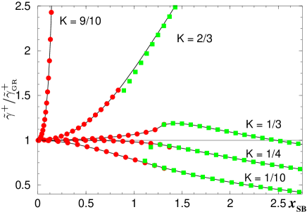
Figure 4: The scaled rate $\tilde{\gamma}^{+}/\tilde{\gamma}_{\rm GR}^{+}$ is plotted versus $x_{\rm SB}$ for various $K<1$. The circles represent the weak-tunneling series and the squares the strong-tunneling expansion. The full curve is the hypergeometric function expression

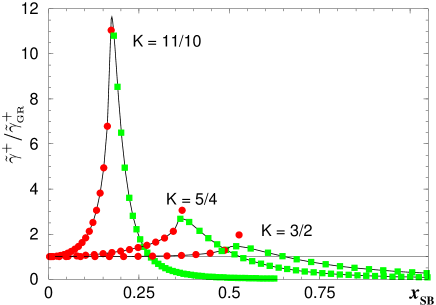
Figure 5: The same scaled rate, but now for various $K>1$.

Next consider large damping $K>1$ and large bias. It is useful to divide the damping regime into the sections $K=p+\kappa$ with $p=1,2,\cdots$ and $0\leq\kappa<1$. In the first step, we change in the integral representation (86) from variable $z$ to variable $t=e^{-i\pi}u_{1/2}z^{K}$. This gives

$$\tilde{\gamma}^{+}={\rm Re}\,\frac{1}{K}\,\frac{\epsilon}{2\pi i}\int_{\cal C}{\rm d}t\,\frac{H(t,u_{1})}{t}\;,$$ (94)

$$\begin{array}[]{rcl}H(t,u_{1})&=&{\displaystyle\sqrt{t-1+e^{i\pi(1+2p)/K}(u_{1}t)^{1/K}}}\\[11.38109pt] &&\quad\quad\quad-\;{\displaystyle\sqrt{t-1+e^{i\pi/K}(u_{1}t)^{1/K}}\;\;.}\end{array}$$ (95)

Second, we expand $H(t,u_{1}$ for small $u_{1}$ and interchange integration and summation. Using (84), we then obtain the asymptotic series as

$$\tilde{\gamma}^{+} = \frac{\epsilon}{2\sqrt{\pi}}\,\sum_{m=1}^{\infty}d_{m}(K)\,\left(\frac{\epsilon}{\epsilon_{0}}\right)^{(2/K-2)m}\;,$$ (96)

$$d_{m}(K) = \frac{(-1)^{m}}{m!}\,\frac{2\,\Gamma(\frac{m}{K})\sin[\,\frac{1+p}{K}m\pi]\sin(\frac{p}{K}m\pi)}{K\,\Gamma[\,\frac{3}{2}+(\frac{1}{K}-1)m\,]}\;.$$

The asymptotic series (96) for the SB model in the regime $K>1$ bears a strong resemblance with the corresponding series of the self-dual Schmid model (81). The powers of $\epsilon/\epsilon_{0}$ follow from those of the perturbative expansion (82) by the substitution $K\to 1/K$, as also do major parts of the coefficient $d_{m}(K)$. However, complete duality is spoilt by the alternating sign and by the sine-factors.

Fig. 5 shows plots of the normalized rate $\tilde{\gamma}^{+}/\tilde{\gamma}^{+}_{\rm GR}$ for $K>1$. The normalized rate goes through a maximum which is shifted to higher $x_{\rm SB}$ when $K$ is increased. At large enough $x_{\rm SB}$, the rate $\tilde{\gamma}^{+}$ falls below the golden rule rate. Hence there is constructive interference of tunneling at small and intermediate $x_{\rm SB}$, and destructive interference in the large tunneling regime.

VI.3 Conjecture on decoherence at $T=0$

So far, we have left aside the damping of the coherent oscillations of the populations. If one aims at calculating frequency and decoherence rate of the oscillation directly, the $\lambda$-dependence of the irreducible clusters discussed above has to be taken into account. The calculation of the respective self-energy and of the decoherence rate has been carried out in special limits, weissbook e.g. for $K\ll 1$. woll89 Here we pose the conjecture that the strong tunneling expansion of the tunneling relaxation rate $\tilde{\gamma}^{+}$, Eq. (88), and the corresponding expansion of the decoherence rate

$$\gamma^{\rm(d)}=\sum_{n=0}^{\infty}\gamma_{n}^{\rm(d)}\;;\qquad\gamma_{n}^{\rm(d)}=\frac{\epsilon_{0}}{2\sqrt{\pi}}\,f_{n}(K)\left(\frac{\epsilon}{\epsilon_{0}}\right)^{2n}$$ (97)

are closely related, viz. that the ratio of the coefficients of these expansions is given by

$$\frac{f_{n}(K)}{b_{n}(K)}=\left\{\begin{array}[]{ll}\frac{1}{2}\;,&K\leq\frac{1}{3}\;,\\[8.53581pt] \sin^{2}[\frac{\pi K(1-2n)}{2(1-K)}]\;,&\frac{1}{3}<K<\frac{1}{2}\;.\\ \end{array}\right.$$ (98)

Equation (98) is in agreement with all exact expressions known in special limits.

The decoherence rate of the unbiased SB model has been calculated within the framework of integrable QFT. lesage98 The respective result (translated into our notation) is

$$\gamma_{0}^{\rm(d)}=\frac{1}{\sqrt{\pi}}{\textstyle\sin^{2}[\frac{\pi K}{2(1-K)}]}\,\frac{\textstyle\Gamma[\frac{K}{2(1-K)}]}{\textstyle\Gamma[\frac{1}{2(1-K)}]}\,\epsilon_{0}$$ (99)

is in correspondence with expressions (98) and (92) for $K\leq\frac{1}{2}$. The relation (98) is known to hold also in the biased case in the regimes $K\ll 1$ and $K$ close to $\frac{1}{2}$. weissbook

These checks suggest that the conjecture (98) holds for the SB model at zero temperature in the regime $0<K\leq\frac{1}{2}$. Upon combining Eqs. (88) - (90) with (98) the weak-bias expansion of the decoherence rate is found as

$$\gamma^{\rm(d)}=\frac{\epsilon_{0}}{2\sqrt{\pi}}\sum_{n=0}^{\infty}{\textstyle\sin^{2}[\frac{\pi K}{1-K}(\frac{1}{2}-n)]}\,c_{n}(K)\left(\frac{\epsilon}{\epsilon_{0}}\right)^{2n}\!\!.$$ (100)

If the conjecture (98) is correct, then the series expression (100) represents the lower bound for decoherence in the SB model in the scaling limit in the regime $0<K\leq\frac{1}{2}$.

VI.4 Leading enhancement at low temperatures

We now extend the discussion to the asymptotic low-temperature regime. The leading thermal correction in the noise amplitude factor $G_{\ell}$ is found from Eq. (27) as

$$G_{\ell}=G_{\ell}(\vartheta=0)\Big{\{}1-K\frac{\pi^{2}}{3}\,\vartheta^{2}\Big{(}\sum_{j=1}^{2\ell-1}p_{j}\tau_{j}\Big{)}^{2}+{\cal O}(\vartheta^{4})\Big{\}}\;,$$

The important point now is to recognize that the annoying term in the round bracket is the bias phase (32). Therefore, this term can be generated by differentiation of the noise integral (31) with respect to the bias. sass90 We thus have, for example,

$$\gamma_{n}^{+}(\epsilon,T)=\left\{1+K\frac{\pi^{2}}{3}\,T^{2}\frac{\partial^{2}}{(\partial\epsilon)^{2}}\right\}\gamma_{n}^{+}(\epsilon,\,T=0)\;.$$ (101)

Corresponding expressions hold for the current $\langle I\rangle_{c}$ and for the moments $\langle I^{(m)}\rangle_{c}$ given in Eq. (76) both in the weak- and strong tunneling regime. Equally, the thermal enhancement of the tunneling rate and the decoherence rate in the SB model has a form analogous to Eq. (101).

We see that the leading enhancement at $T\ll\epsilon$ varies with $T^{2}$. The power 2 is a signature of Ohmic dissipation. In addition the prefactor is universally given by the curly bracket with the second order differential expression in Eq. (101). The universal form is closely related to the Wilson ratio in the AKM, in which the specific heat is related to the static susceptibility. sass90 The physical origin of the $T^{2}$ enhancement is the low-frequency thermal noise of the dissipation.grabert88

VII Conclusion

In summary, we uncovered exact functional relations between perturbative integrals occuring in the nonequilibrium Keldysh approach applied to the Schmid and the SB model at $T=0$. With that and with use of the correspondence of the Schmid with the BSG model, we found agreement between the results of the Keldysh approach and the thermodynamic Bethe ansatz for the BSG model. As a second result, we discovered exact functional relations between the rates in the Schmid model and the partial rates in the SB model. Starting out from the perturbative series obtained by use of the functional relations, we put up an exact integral representation for the tunneling rate in the SB model, from where we derived the asymptotic or strong-backscattering expansion. Thirdly, we conjectured and checked a relation between the relaxation and the decoherence rate in the SB model. Finally, we calculated the leading thermal enhancement of the transport and of all statistical fluctuations and found universal behaviour.

Our results are relevant, e.g., to charge transfer, macroscopic quantum coherence (qubits), and diverse quantum impurity problems.

References

• (1) U. Weiss, Quantum Dissipative Systems (World Scientific, Singapore, 2nd edition, 1999).
• (2) P. Fendley and H. Saleur, Phys. Rev. Lett. 75, 4492 (1995).
• (3) P. Fendley, F. Lesage, and H. Saleur, J. Stat. Phys. 85, 211 (1996).
• (4) A.J. Leggett et al., Rev. Mod. Phys. 59, 1 (1987).
• (5) A. Schmid, Phys. Rev. Lett. 51, 1506 (1983).
• (6) R. de-Picciotto et al., Nature 389, 162 (1997).
• (7) S. Roddaro et al., Phys. Rev. Lett. 90, 46805 (2003).
• (8) J. Kondo, in Fermi Surface Effects, Vol. 77 of Springer Series in Solid State Sciences, eds. J. Kondo and A. Yoshimori (Springer, Berlin, 1988).
• (9) A.M. Tsvelik and P.B. Wiegmann, Adv. Physics, 32, 453 (1983).
• (10) P. Fendley, A. Ludwig, and H. Saleur, Phys. Rev. B 52, 8934 (1995).
• (11) H. Saleur and U. Weiss, Phys. Rev. B 63 201302(R) (2001).
• (12) W. Zwerger, Phys. Rev. B 35, 4737 (1987).
• (13) M. Sassetti, H. Schomerus, and U. Weiss, Phys. Rev. B 53, R2914 (1996).
• (14) M.P.A. Fisher and W. Zwerger, Phys. Rev. B 32, 6190 (1985).
• (15) U. Weiss, Solid. State Comm. 100, 281 (1996).
• (16) P. Fendley and H. Saleur, Phys. Rev. Lett. 81, 2518 (1998).
• (17) N.M. Temme, Special Functions, (Wiley, New York, 1996).
• (18) U. Weiss and M. Wollensak, Phys. Rev. Lett. 62, 1663 (1989).
• (19) F. Lesage and H. Saleur, Phys. Rev. Lett. 80, 4370 (1998).
• (20) M. Sassetti and U. Weiss, Phys. Rev. Lett. 65, 2262 (1990).
• (21) J.M. Martinis and H. Grabert, Phys. Rev. B 38, 2371 (1988).