[

Tunneling through two resonant levels: fixed points and conductances

Abstract

We study point contact tunneling between two leads of a Tomonaga-Luttinger liquid through two degenerate resonant levels in parallel. This is one of the simplest cases of a quantum junction problem where the Fermi statistics of the electrons plays a non-trivial role through the Klein factors appearing in bosonization. Using a mapping to a ‘generalized Coulomb model’ studied in the context of the dissipative Hofstadter model, we find that any asymmetry in the tunneling amplitudes from the two leads grows at low temperatures, so that ultimately there is no conductance across the system. For the symmetric case, we identify a non-trivial fixed point of this model; the conductance at that point is generally different from the conductance through a single resonant level.

]

The calculation of conductances of quantum wires and dots continues to be of major interest, as the sophistication in the fabrication of semiconductor heterostructures and carbon nanotubes increases. Tunneling through barriers and quantum dots are now amenable to sophisticated controls that allow tunneling through specific levels in quantum dot. On the theoretical side, several studies of low dimensional systems have probed the effects of strong correlations which often lead to novel features [2].

The motivation for this work is that tunneling through two resonant levels appears to be the simplest set-up in which the Fermi statistics of the electrons that tunnel through the levels play a non-trivial role and lead to a non-trivial fixed point. Further, using quantum dots in parallel, the set-up can also be experimentally realized.

In this paper, we study a model of quantum tunneling of spinless electrons between two leads through two parallel resonant levels which are degenerate. The set-up is schematically shown in Fig. 1. A simple experimental realization of the model is shown in Fig. 2; the leads labeled $A$ and $B$ are connected to two quantum dots labeled 1 and 2 in parallel, with both the dots having been tuned to conduct through a single level. A magnetic flux can also be passed through the ring allowing for arbitrary phases in the tunneling amplitudes.

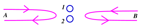
FIG. 1.: Schematics of a two-lead two resonant level multiple tunneling setup.

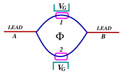
FIG. 2.: Possible experimental realization of tunneling through two resonant levels, using two quantum dots in parallel which are tuned to resonance by gate voltages. Phases in the tunneling amplitudes can be introduced through a non-zero magnetic flux through the ring.

The bosonized action for the two disconnected wires in Fig. 1 is given in imaginary time by [2]

$$S_{0}~{}=~{}\frac{1}{2g}~{}\int d\tau~{}[\int_{-\infty}^{0}dx(\partial_{\mu}\phi_{A})^{2}+\int_{0}^{\infty}dx(\partial_{\mu}\phi_{B})^{2}]~{}.$$ (1)

Here $\phi_{a}$ ($a=A,B$) is related to the electron annihilation operator on the $a^{th}$ wire as $\psi_{a}\sim\eta_{a}e^{i\phi_{a}/{\sqrt{2}}}$. The Klein factors $\eta_{a}$ are needed to enforce Fermi statistics, i.e., $\{\eta_{a},\eta_{b}\}=2\delta_{ab}$. The $\eta_{a}$’s can be chosen to be two of the Pauli matrices; hence $\eta_{a}^{\dagger}=\eta_{a}$.

The two charge states at each of the resonant levels at the origin are represented by spin 1/2 degrees of freedom. The spin raising and the spin lowering operators $S_{i}^{\pm}$ are the creation and annihilation operators for an electron at the resonant level $i$. The tunneling between the leads and the resonant levels is described by

$$H_{t} = t_{1A}S_{1}^{+}\eta_{A}e^{i\phi_{A}/{\sqrt{2}}}~{}+~{}t_{1B}S_{1}^{+}\eta_{B}e^{i\phi_{B}/{\sqrt{2}}}$$ (2)

$$+ t_{2A}S_{2}^{+}\eta_{A}e^{i\phi_{A}/{\sqrt{2}}}~{}+~{}t_{2B}S_{2}^{+}\eta_{B}e^{i\phi_{B}/{\sqrt{2}}}+h.c.$$ (3)

Here $t_{(1B,2B)}$ are the amplitudes for the electrons to tunnel to the two resonant levels 1 and 2 from the right lead $B$, and $t_{(1A,2A)}$ are the tunneling amplitudes from the left lead $A$. We have been most general here and allowed for asymmetric tunnelings. If the tunneling was symmetric between the two leads, we would have $t_{1A,2A}=t_{1B,2B}$. We have also allowed for different tunneling amplitudes to the two levels; $t_{1A,1B}$ need not be equal to $t_{2A,2B}$. Note that in general, $t_{ia}$ ($i=1,2$ and $a=A,B$) may be complex; this will take care of the phases that may be generated by a flux through the ring. However, for the calculations below, we will assume that all the $t_{ia}$ are real.

It is easy to check that the scaling dimensions of all the tunneling operators in Eq. (3) are just $1/(2g)$. So for $g<1/2$, it is irrelevant and the decoupled fixed point is stable. However, for $g>1/2$, the decoupled fixed point is unstable; one would then like to find the stable fixed point(s) of the theory.

To solve the problem, we need to be able to calculate correlation functions involving any string of operators $e^{i\phi_{a}}$. In the absence of Klein factors, this would be trivial, since the $\phi_{a}$ are just free bosonic fields. The presence of the Klein factors gives rise to non-trivial phases.

We first study the problem with a single resonant level to illustrate our method, i.e., we set $t_{2A}=t_{2B}=0$. The partition function is given by

$$Z~{}=~{}\int{\cal D}\phi_{A}{\cal D}\phi_{B}~{}e^{-S(\phi_{A},\phi_{B})}$$ (4)

where $S=S_{0}+\int d\tau dxH_{t}$. On expanding this, terms involving multiple tunnelings of the electrons will be generated. Following Ref. [3], we can map the problem to a one-dimensional Coulomb gas of logarithmically interacting charges by classifying the different tunnelings in terms of the charges $q_{i}=m_{i}-n_{i}$ and $r_{i}=m_{i}+n_{i}$. Here $m_{i}$ and $n_{i}$ denote the charges transferred to the resonant level from the left lead and right lead respectively. Thus, $q_{i}$ is the total charge transferred from the left lead to the right lead in any process, and $r_{i}$ is the change in the charge on the resonant level in any process. The four different kinds of tunneling events can be classified in terms of $q_{i}$ and $r_{i}$ as follows.

1. tunnel from lead $A$ to resonant level: $r_{i}=1,q_{i}=1$.

2. tunnel from resonant level to lead $A$: $r_{i}=-1,q_{i}=-1$.

3. tunnel from lead $B$ to resonant level: $r_{i}=1,q_{i}=-1$.

4. tunnel from resonant level to lead $B$: $r_{i}=-1,q_{i}=1$.

Furthermore, events 1 and 2 carry Klein factors of $\eta_{A}$, while events 3 and 4 carry a Klein factor of $\eta_{B}$. Let $N_{k}$ (where $k=1,2,3,4$) represent the number of each of the above events in the partition function.

Without Klein factors, the order of the tunnelings does not matter; if we also assume that the resonant level can accommodate any number of electrons, it is easy to see that an arbitrary term in the expansion of the partition function can be written as

$$(t_{1A})^{N_{1}+N_{2}}(t_{1B})^{N_{3}+N_{4}}<{S_{1}^{+}}^{N_{1}}~{}{S_{1}^{-}}^{N_{2}}~{}{S_{1}^{+}}^{N_{3}}~{}{S_{1}^{-}}^{N_{4}}>$$ (5)

$$<e^{i\phi_{A}/{\sqrt{2}}}\cdot\cdot~{}N_{1}~{}{\rm times}~{}\times~{}e^{-i\phi_{A}/{\sqrt{2}}}\cdot\cdot~{}N_{2}~{}{\rm times}~{}\times$$ (6)

$$\quad e^{i\phi_{B}/{\sqrt{2}}}\cdot\cdot~{}N_{3}~{}{\rm times}~{}\times~{}e^{-i\phi_{B}/{\sqrt{2}}}\cdot\cdot~{}N_{4}~{}{\rm times}>.$$ (7)

This correlation function is non-zero only when $N_{1}=N_{2}$ and $N_{3}=N_{4}$; then the spin terms just give unity. So the full partition function is given by

$$Z~{}=~{}\sum_{N_{1},N_{3}}~{}(t_{1A})^{2N_{1}}(t_{1B})^{2N_{3}}\int d\tau_{1}d\tau_{2}....d\tau_{N}$$ (8)

$$\quad~{}~{}<e^{im_{1}\phi_{A}/{\sqrt{2}}}e^{im_{2}\phi_{A}/{\sqrt{2}}}\cdots e^{in_{1}\phi_{B}/{\sqrt{2}}}e^{in_{2}\phi_{B}/{\sqrt{2}}}\cdots>,$$ (9)

where $m_{i}=\pm 1$, $\sum_{i}|m_{i}|=2N_{1}$, $n_{i}=\pm 1$, $\sum_{i}|n_{i}|=2N_{3}$. The total number of events is $N=2N_{1}+2N_{3}$. The correlation functions can easily be calculated since the bosons are free. Using

$$<e^{im_{i}\phi_{A}(\tau_{i})/{\sqrt{2}}}e^{im_{j}\phi_{A}(\tau_{j})/{\sqrt{2}}}>=e^{{1\over{2g}}m_{i}m_{j}\ln(\tau_{i}-\tau_{j})^{2}/\tau_{c}^{2}}~{},$$ (11)

where $\tau_{c}$ is an infra-red cutoff, one can see that the resulting partition function is identical to that of two independent Coulomb gases, with charges $m_{i}$ and $n_{i}$. The partition function can be written as

$$Z = \sum_{m_{i},n_{i}}~{}(t_{1A})^{|m_{i}|}(t_{1B})^{|n_{i}|}\int d\tau_{1}d\tau_{2}...d\tau_{N}$$ (13)

$$\quad\prod_{i<j}e^{{1\over{2g}}(m_{i}m_{j}+n_{i}n_{j})\ln(\tau_{i}-\tau_{j})^{2}/\tau_{c}^{2}~{}}~{},$$

where $N=\sum_{i}(|m_{i}|+|n_{i}|)$.

For the fermionic model (with Klein factors present), the ordering of the tunnelings becomes important since not more than one electron can sit on a resonant level. (We are considering the case of spinless electrons here). This means that the tunnelings on to and off the resonant level have to alternate in time. In other words, any chain of events must satisfy the following three constraints:

(i) $\sum_{i}q_{i}=0$,  (ii) $\sum_{i}r_{i}=0$, and

(iii) the $r_{i}$ alternate in sign.

Does the presence of two Klein factors lead to non-trivial phases in the partition function? The answer is no; this can be understood as follows. First, we note that for any pair of events $i$ and $j$, the exchange of the two Klein factors leads to a phase,

$$\eta_{i}\eta_{j}=\eta_{j}\eta_{i}~{}e^{i(\pi/2)(q_{i}r_{j}-q_{j}r_{i}){\rm sign}(\tau_{i}-\tau_{j})}~{}.$$ (14)

(Here ${\rm sign}(\tau)=1$ for $\tau>0$ and $-1$ for $\tau<0$). Eq. (14) can easily be checked for the events of type 1 to 4 listed above. For instance, 1 followed by 2 gives a phase of 1, whereas 1 followed by 4 gives a phase of $-1$. Eq. (14) suggests that for one particular ordering of two events, it is useful to introduce a factor whose phase is equal to half the exchange phase given in that equation, namely,

$$P_{ij}~{}=~{}e^{i(\pi/4)(q_{i}r_{j}-q_{j}r_{i}){\rm sign}(\tau_{i}-\tau_{j})}~{}.$$ (15)

One can use Eq. (14) to repeatedly exchange Klein factors so as to eventually bring pairs of identical Klein factors next to each other; the product of such a pair is equal to the identity matrix since each Klein factor is given by a Pauli matrix. In this way, one can show that the total phase factor for any term in the partition function can be written purely as a phase factor, namely,

$$P~{}=~{}\prod_{i<j}P_{ij}~{}.$$ (16)

Now, using the three conditions stated above, it is easy to check that $P=1$. This is crucially dependent on condition (iii) which says that $r_{i}$ has to alternate. Hence, the phases due to the fermionic nature of the electrons do not play a non-trivial role in this case. So the computation of the correlation functions can be done as for the case without the Klein factors.

To implement the constraints (i)-(iii), it is more convenient to rewrite the partition function in Eq. (13) terms of $r_{i}$ and $q_{i}$; we obtain

$$Z = \sum_{N}\sum_{q_{i}}(t_{1A})^{(1+q_{i}r_{i})/2}(t_{1B})^{(1-q_{i}r_{i})/2}\int d\tau_{1}d\tau_{2}...d\tau_{N}$$ (18)

$$\quad\prod_{i<j}e^{{1\over{4g}}(r_{i}r_{j}+q_{i}q_{j})\ln(\tau_{i}-\tau_{j})^{2}/\tau_{c}^{2}}~{}.$$

Note that we do not need the sum over $r_{i}$, because once $r_{1}$ is fixed, the rest are fixed by the alternation rule. This agrees with the result in Ref. [3] for the double barrier case, which is similar to the case of the single resonant level, as expected.

The Coulomb gas partition function can then be studied using the renormalization group (RG) method as done in Ref. [3]. Let us first discuss the symmetric case $t_{1A}=t_{1B}$. For $g>1/2$, it was shown in Ref. [3] that the tunneling amplitudes for a double barrier structure (which may be expected to have the same behavior as the single resonant level that we are considering) grow under the RG transformation, eventually leading to a ‘healing’ between the leads $A$ and $B$. We will demonstrate this below. On the other hand, for $g<1/2$, the tunneling amplitude $t_{1A}=t_{1B}$ decreases under RG as mentioned earlier; the stable fixed point then is the ‘cut’ wire with zero transmission between the two leads. The conductance is given by $ge^{2}/h$ if the wire is healed, and zero if the wire is cut. For the asymmetric case $t_{1A}\neq t_{1B}$, the situation is somewhat different. One finds the wire gets healed and the conductance is $ge^{2}/h$ if $g>1$, while the wire is cut and the conductance is zero if $g<1$ [3].

We now consider the case of two resonant levels. The main difference from the earlier analysis is that we now have to consider tunnelings to resonant level 1 and level 2 independently. We define $r_{i}$ as the total charge transferred to resonant level 1, $s_{i}$ as the total charge transferred to resonant level 2, and $q_{i}$ as the charge transferred from lead $A$ to lead $B$. Then the eight possible tunneling events and their charge assignments are as follows.

1. tunnel from lead $A$ to level 1: $r_{i}=1,s_{i}=0,q_{i}=1$.

2. tunnel from level 1 to lead $A$: $r_{i}=-1,s_{i}=0,q_{i}=-1$.

3. tunnel from lead $B$ to level 1: $r_{i}=1,s_{i}=0,q_{i}=-1$.

4. tunnel from level 1 to lead $B$: $r_{i}=-1,s_{i}=0,q_{i}=1$.

5. tunnel from lead $A$ to level 2: $r_{i}=0,s_{i}=1,q_{i}=1$.

6. tunnel from level 2 to lead $A$: $r_{i}=0,s_{i}=-1,q_{i}=-1$.

7. tunnel from lead $B$ to level 2: $r_{i}=0,s_{i}=1,q_{i}=-1$.

8. tunnel from level 2 to lead $B$: $r_{i}=0,s_{i}=-1,q_{i}=1$.

Events 1-2 and 5-6 have Klein factors $\eta_{A}$, while the others have Klein factors $\eta_{B}$. Let us again denote the number of events of type $i$ as $N_{i}$. It is easy to check that the correlation function of such a set of events will be non-zero only if $N_{1}+N_{5}=N_{2}+N_{6}$ and $N_{3}+N_{7}=N_{4}+N_{8}$. The partition function for this model can now be computed in the same way that it was computed for the single resonant level case. However, as we shall see below, this model will get mapped to a different Coulomb gas model which has charges $r_{i}$, $s_{i}$ and $q_{i}$ and non-trivial phases.

Just as before, Fermi statistics implies that for any chain of events,

(i) $\sum_{i}q_{i}=0$, (ii) $\sum_{i}r_{i}=\sum_{i}s_{i}=0$, and

(iii) non-zero values of $r_{i}$ and $s_{i}$ alternate in sign.

We now define $R_{i}=r_{i}+s_{i}$, and note that it can only take the values $\pm 1$. Overall charge neutrality implies that $\sum_{i}R_{i}=0$, but $R_{i}$ does not have to alternate in sign (unlike $r_{i}$ in the earlier model with only one resonant level). One finds that the phase can once again be written as

$$P_{ij}=e^{i(\pi/4)(q_{i}R_{j}-q_{j}R_{i}){\rm sign}(\tau_{i}-\tau_{j})}~{}.$$ (19)

However, since the $R_{i}$ do not have to alternate, the total phase $P$ in a chain of events in the partition function does not always have to be 1; it can sometimes be $-1$. This can be seen if we consider the chain of events 1,4,6,7 which contains the string $\eta_{A}\eta_{B}\eta_{A}\eta_{B}=-1$. Hence, this model clearly has non-trivial phases. This means that if we want to map it to a Coulomb gas problem, we need to worry about phases. That is, in the partition function, along with the logarithms which appear due to the contraction of the pairs of $\phi$ fields, we also need to include the phases which appear from the Klein factors. Note that the above phase occurs even in the absence of a magnetic flux through the ring, i.e., even when the tunneling amplitudes are real. When the tunnelings are complex (due to a flux through the ring), we will have extra phases.

Let us write the partition function including the phases as follows:

$$Z = \sum_{N}\sum_{R_{i},q_{i}}~{}(\prod_{i}t_{ia})~{}\int d\tau_{1}d\tau_{2}...d\tau_{N}$$ (21)

$$\quad\prod_{i<j}P_{ij}~{}e^{{1\over{4g}}(R_{i}R_{j}+q_{i}q_{j})\ln(\tau_{i}-\tau_{j})^{2}/\tau_{c}^{2}}~{},$$

where $t_{ia}$ can denote $t_{1A},t_{1B},t_{2A}$ or $t_{2B}$. Eq. (21) looks very similar to Eq. (18) for the model with a single resonance level except for the alternating constraint and the presence of the phases $P_{ij}$.

Fortunately, the above problem with the phases can be mapped to a ‘generalized Coulomb gas model’ studied in the context of the dissipative Hofstadter model, provided that $t_{1A}=t_{2A}=t_{A}$ and $t_{1B}=t_{2B}=t_{B}$. This is a model of free bosons with a ‘magnetic field’ at the boundary, and it has been studied in detail in Ref. [4, 5].

Let us introduce the model studied in Ref. [4] and show that the expansion of its partition function agrees with the expansion of the partition function for the above model with two resonant levels, under a certain identification of the parameters. They introduced a model for the quantum motion of a single particle in the presence of a magnetic field, a periodic potential and dissipation; the model is described by the action

$$S = {1\over 2}\int d\omega~{}[~{}\alpha|\omega|\delta_{\mu\nu}~{}+~{}\beta\omega\epsilon_{\mu\nu}~{}]~{}X_{\mu}(\omega)X_{\nu}(\omega)$$ (23)

$$+\int d\tau~{}[t_{A}e^{i{\bf K}_{1}\cdot{\bf X}(\tau)}+t_{B}e^{i{\bf K}_{2}\cdot{\bf X}(\tau)}+h.c.]~{},$$

where $\mu,\nu=1,2$, $\epsilon_{12}=-\epsilon_{21}=1$, and $\epsilon_{11}=\epsilon_{22}=0$. Here $\alpha$ and $\beta$ are related to the dissipation and the magnetic field respectively. The potential term is defined in terms of two vectors ${\bf K}_{1}=(1,0)$ and ${\bf K}_{2}=(0,1)$; these vectors define a rectangular basis for a two-dimensional plane defined by ${\bf X}=X_{1}{\bf K}_{1}+X_{2}{\bf K}_{2}$. The quadratic part of the above action leads to the propagator

$$D_{\mu\nu}= <X_{\mu}(\tau_{1})X_{\nu}(\tau_{2})>$$ (24)

$$= -~{}{\alpha\over\alpha^{2}+\beta^{2}}~{}\delta_{\mu\nu}~{}\ln(\tau_{1}-\tau_{2})^{2}/\tau_{c}^{2}$$ (26)

$$+~{}i\pi{\beta\over\alpha^{2}+\beta^{2}}~{}\epsilon_{\mu\nu}~{}{\rm sign}(\tau_{1}-\tau_{2})~{}.$$

The unusual part of the above propagator is the second term or phase term, which exists only in the presence of the second term in the action Eq. (23); this is a ‘magnetic field’ term and it is antisymmetric in the indices $\mu$ and $\nu$. If we now expand the partition function in powers of the perturbations $t_{i}$, we get terms of the form

$$(\prod_{i}t_{i})\int d\tau_{1}d\tau_{2}\dots...d\tau_{n}$$ (27)

$$<e^{i{\bf L}_{1}\cdot{\bf X}(\tau_{1})}<e^{i{\bf L}_{2}\cdot{\bf X}(\tau_{2})}\dots<e^{i{\bf L}_{n}\cdot{\bf X}(\tau_{n})}>$$ (28)

$$=(\prod_{i}t_{i})\int d\tau_{1}d\tau_{2}\dots...d\tau_{n}\delta(\sum_{i}{\bf L}_{i})$$ (29)

$$\exp~{}[{\alpha\over\alpha^{2}+\beta^{2}}~{}\sum_{i<j}{\bf L}_{i}\cdot{\bf L}_{j}{\rm ln}(\tau_{i}-\tau_{j})^{2}/\tau_{c}^{2}$$ (30)

$$-i\pi~{}{\beta\over\alpha^{2}+\beta^{2}}~{}\sum_{i<j}{\bf L}_{i}\times{\bf L}_{j}{\rm sign}(\tau_{i}-\tau_{j})]$$ (31)

at the $n^{th}$ order. Here each ${\bf L}_{i}$ is one of the four vectors $\pm{\bf K}_{1,2}$.

For the eight tunneling events described above, let us associate the vector ${\bf K}_{1}$ with events 1 and 5, $-{\bf K}_{1}$ with events 2 and 6, ${\bf K}_{2}$ with events 3 and 7, and $-{\bf K}_{2}$ with events 4 and 8. Then we find that for any pair of events, $R_{i}R_{j}+q_{i}q_{j}=2{\bf K}_{i}\cdot{\bf K}_{j}$ and $q_{i}R_{j}-q_{j}R_{i}=-2{\bf K}_{i}\times{\bf K}_{j}$. Hence the term in Eq. (31) matches a similar term in the partition function Eq. (21) of the resonant tunneling model if we equate

$$\frac{\alpha}{\alpha^{2}+\beta^{2}} = \frac{1}{2g}~{},$$ (32)

$$\frac{\beta}{\alpha^{2}+\beta^{2}} = n~{}-~{}\frac{1}{2}~{},$$ (33)

where $n$ is some fixed integer. This implies that

$$\alpha = \frac{2g}{1~{}+~{}(2n-1)^{2}g^{2}}~{},$$ (34)

$$\beta = \frac{2(2n-1)g^{2}}{1~{}+~{}(2n-1)^{2}g^{2}}~{}.$$ (35)

Different values of the integer $n$ describe different field theories for the $X_{i}$ in Eq. (23), but they describe the same resonant level model. As we have seen earlier, the tunneling term is irrelevant if $g<1/2$ (i.e., inside the circle $\alpha^{2}+\beta^{2}=\alpha$ in the ($\alpha,\beta$) plane), and is relevant for $g>1/2$ (outside the circle $\alpha^{2}+\beta^{2}=\alpha$). Thus we flow towards the strong tunneling limit if $g>1/2$.

We now begin at the opposite end and study the stability of the infinite tunneling (healed) limit. For $t_{A},t_{B}\rightarrow\infty$ in Eq. (23), the fields $X_{1}$ and $X_{2}$ get pinned at the minima of the potential. These minima form a square lattice with lattice spacing $2\pi$. The fluctuations around these minima are given by instantons which tunnel from one minimum to another [4]. The scaling dimension of these fluctuations are given by the square of the lattice spacing (in units of $2\pi$) multiplied by $\alpha$ [4, 6]. Hence the scaling dimension is given by

$$\Delta_{n}~{}=~{}\frac{2g}{1~{}+~{}(2n-1)^{2}g^{2}}~{}.$$ (36)

We see that this is always less than 1 except when $g=1$ and $n=0$ or 1. Thus the strong tunneling limit is always unstable, except when $g=1$ (which describes non-interacting electrons); we shall discuss this special case later. We therefore conclude that healing by resonant tunneling through two levels is generically not possible.

However, let us now return to the case of resonant tunneling through only one wire [3], namely, $t_{2A}=t_{2B}=0$. Then there are no phases as we saw earlier. A comparison between Eqs. (18) and (31) shows that the parameters $\alpha$ and $\beta$ satisfy

$$\frac{\alpha}{\alpha^{2}+\beta^{2}} = \frac{1}{2g}~{},$$ (37)

$$\frac{\beta}{\alpha^{2}+\beta^{2}} = n~{}.$$ (38)

This implies that

$$\alpha = \frac{2g}{1~{}+~{}4n^{2}g^{2}}~{},$$ (39)

$$\beta = \frac{4ng^{2}}{1~{}+~{}4n^{2}g^{2}}~{}.$$ (40)

In the limit of infinite tunneling, the fields $X_{1}$ and $X_{2}$ again get pinned at the points of a two-dimensional lattice with lattice spacing $2\pi$. The scaling dimension of the instanton fluctuations is now given by

$$\Delta_{n}~{}=~{}\frac{2g}{1~{}+~{}4n^{2}g^{2}}~{}.$$ (41)

The maximum possible value of this occurs at $n=0$, when the scaling dimension is $2g$. Then the infinite tunneling limit is stable for $g>1/2$ and unstable for $g<1/2$. This is the result in Ref. [3], except for some modifications in the region $1/4<g<1/2$ (these arise because they deal with a double barrier system, not a single resonant level, and hence have other possibilities of back-scattering). Ref. [3] also shows that the conductance is given by $ge^{2}/h$ if $g>1/2$.

A better understanding of the two-resonant level model can be obtained from the RG equations for the theory defined in Eq. (23). Using the method described in Ref. [5], one can derive the RG equations to third order in the tunneling amplitudes $t_{A}$ and $t_{B}$. Using Eqs. (33), we find that for any integer $n$,

$${dt_{A}\over d\ln L} = (1~{}-~{}{1\over 2g}~{})~{}t_{A}~{}-~{}{t_{A}t_{B}^{2}\over 4\pi^{2}}~{},$$ (42)

$${dt_{B}\over d\ln L} = (1~{}-~{}{1\over 2g}~{})~{}t_{B}~{}-~{}{t_{B}t_{A}^{2}\over 4\pi^{2}}~{},$$ (43)

where $L$ denotes the length scale. For $g>1/2$, there is a stable fixed point for non-zero values of the $t_{a}$ given by $t_{A}^{2}=t_{B}^{2}=t_{c}^{2}$ where

$$t_{c}^{2}~{}=~{}4\pi^{2}~{}(1-~{}{1\over 2g}~{})~{}.$$ (44)

The location of this fixed point moves closer to zero, the closer we get to $g=1/2$. So this third order RG result is trustworthy for small values of $t_{c}$ which occur close to $g=1/2$. Since we expect the conductance of the system to be proportional to the square of the tunneling amplitude (if the amplitude is weak), we find that

$$G~{}\sim~{}\frac{e^{2}}{h}~{}t_{c}^{2}~{}\sim~{}\frac{e^{2}}{h}~{}(~{}1~{}-~{}{1\over 2g}~{})~{}.$$ (45)

Note the non-linear dependence on $g$ at this point, similar to the non-linear dependence obtained in Ref. [6].

Eqs. (43) imply that

$${d(t_{A}^{2}-t_{B}^{2})\over d\ln L}~{}=~{}(~{}2~{}-~{}\frac{1}{g}~{})~{}(t_{A}^{2}-t_{B}^{2})~{}.$$ (46)

For $g>1/2$, this implies that any asymmetry in the amplitudes grows with the length scale. Hence, if $t_{A}^{2}\neq t_{B}^{2}$ to begin with, they will become increasingly more unequal. One can then show from Eqs. (43) that eventually the larger amplitude will flow to infinity while the smaller amplitude will flow to zero.

We thus see that if $g>1/2$, a non-zero conductance through two levels in parallel is not a stable situation. If we fine tune the tunneling amplitudes so that $t_{1A}=t_{2A}=t_{A}$ and $t_{1B}=t_{2B}=t_{B}$ are equal, then the system flows to an intermediate fixed point (IFP). But if we begin with generic values of $t_{A}$ and $t_{B}$ which are not equal, then one of them eventually grows to infinity while the other goes to zero. The conductance between the two leads is then zero in the long distance limit. A schematic RG flow diagram in the $(t_{A},t_{B})$ plane is shown in Fig. 3.

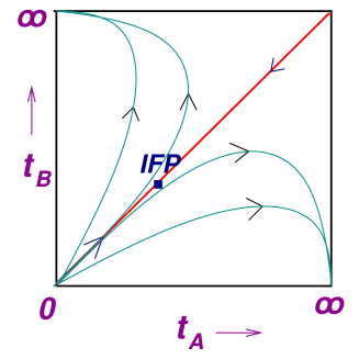
FIG. 3.: Schematic picture of the renormalization group flow in the $(t_{A},t_{B})$ plane. An intermediate fixed point is shown on the $t_{A}=t_{B}$ line.

The symmetry between the two leads (channels) is not ‘protected’ by any conservation law in our model. In order to access the non-trivial fixed point experimentally, one may therefore need to consider a different set-up in which the two channels are labeled by spin up and spin down [7]; this would give rise to a robust symmetry in the absence of a magnetic field.

For the non-interacting case given by $g=1$, we can compute the conductance in terms of the parameters $t_{A}$ and $t_{B}$ defined in the previous paragraph. We use the equation of motion method [8]. We first ‘unfold’ the left and right half-lines to full lines, and define the electron fields $\psi_{a}(x,\tau)$, where $a=A,B$ and $-\infty<x<\infty$. The incoming and outgoing fermion fields are given by $\psi_{a}(0-,\tau)$ and $\psi_{a}(0+,\tau)$ respectively. The creation and annihilation operators for the two resonant levels (which lie at $x=0$) are defined as $d_{i}(\tau)$ and $d_{i}^{\dagger}(\tau)$, where $i=1,2$. In terms of these fields, the action for $g=1$ is given by

$$S = \int d\tau~{}[~{}\sum_{i}d_{i}^{\dagger}\partial_{\tau}d_{i}+\int_{-\infty}^{\infty}dx~{}\{~{}\sum_{a}~{}\psi_{a}^{\dagger}(\partial_{\tau}+i\partial_{x})\psi_{a}$$ (48)

$$\quad\quad\quad\quad\quad+~{}\delta(x)~{}\sum_{a,i}~{}t_{a}~{}(\psi_{a}^{\dagger}d_{i}+d_{i}^{\dagger}\psi_{a})~{}\}~{}]~{}.$$

The equations of motion for this system are:

$$[~{}\partial_{\tau}~{}+~{}i~{}\partial_{x}~{}]~{}\psi_{a}(x,\tau)~{}+~{}\delta(x)~{}t_{a}~{}\sum_{i}~{}d_{i}(\tau) = 0~{},$$ (49)

$$\partial_{\tau}d_{i}(\tau)~{}+~{}\sum_{a}~{}t_{a}\psi_{a}(0,\tau) = 0~{}.$$ (50)

Here $\psi_{a}(0,\tau)=[\psi_{a}(0+,\tau)+\psi_{a}(0-,\tau)]/2$. We integrate the first equation in (50) from $x=0-$ to $x=0+$, and then Fourier transform in time to obtain

$$i~{}[~{}\psi_{a}(0+,\omega)~{}-~{}\psi_{a}(0-,\omega)~{}]~{}+~{}t_{a}~{}\sum_{i}~{}d_{i}(\omega) = 0,$$ (51)

$$\omega d_{i}(\omega)~{}+~{}\sum_{a}~{}t_{a}\psi_{a}(0,\omega) = 0.$$ (52)

We now eliminate the operators $d_{i}(\omega)$ and relate the outgoing fermion fields to the incoming fermion fields through a scattering matrix $S$, namely, $\psi_{a}(0+,\omega)=\sum_{b}S_{ab}\psi_{b}(0-,\omega)$. In the limit $\omega\rightarrow 0$ (dc conductance), we find that $S_{AA}=-S_{BB}=-(t_{A}^{2}-t_{B}^{2})/(t_{A}^{2}+t_{B}^{2})$, and $S_{AB}=S_{BA}=-2t_{A}t_{B}/(t_{A}^{2}+t_{B}^{2})$. The conductance is given by $e^{2}/h$ times $|S_{AB}|^{2}$. Thus the conductance depends on the precise values of $t_{A}$ and $t_{B}$ if $g=1$.

The non-interacting case may be exceptional in that the conductance is a continuous function of the tunneling amplitudes $t_{A}$ and $t_{B}$. For the interacting case $g\neq 1$ (and larger than 1/2), we saw above that the symmetric model ($t_{A}=t_{B}$) and the asymmetric model ($t_{A}\neq t_{B}$) have different fixed points, and the conductance at large length scales can take only two different values, i.e., a finite value given in Eq. (45) and zero respectively.

A comparison between the symmetric one-resonant level model ($t_{1A}=t_{1B}\neq 0$, and $t_{2A}=t_{2B}=0$) and the symmetric two-resonant level model ($t_{1A}=t_{1B}=t_{2A}=t_{2B}\neq 0$) shows that for $g$ slightly larger than 1/2, the conductance in the former case (where only one level contributes) is larger than in the latter case (where both levels contribute). This probably happens because, in the two-resonant level model, the phase factors $P_{ij}$ in Eq. (21) lead to destructive interference between different series of tunneling events.

It is straightforward to extend the above analysis to the case in which $t_{1A}=t_{1B}$ and $t_{2A}=t_{2B}$ are complex. A more difficult problem would be to study the general two-resonant level model in which the four tunneling amplitudes $t_{ia}$ are all different from each other and are complex. (Such a generalization would allow one to examine the case in which there is a magnetic flux through the centre of the system as indicated in Fig. 2). However, it does not seem possible at present to study such a general model using the known Coulomb gas approach which, as mentioned above, requires one to assume that $t_{1A}=t_{2A}$ and $t_{1B}=t_{2B}$.

To summarize, we have shown that a Tomonaga-Luttinger liquid tunneling through two resonant levels has a non-trivial fixed point at long distances if $g>1/2$ and the tunneling amplitudes from the two leads are equal. If the two amplitudes are not equal, then the model flows to a different fixed point in which one of the tunneling amplitudes and, therefore, the conductance is zero. Thus an asymmetry between the two leads is a relevant perturbation which grows at long distances. This behavior is similar in spirit to that of the one-impurity two-channel Kondo model in which an asymmetry between the couplings of the two channels to a spin-1/2 magnetic impurity is a relevant perturbation which drives the system to a fixed point that is very different from that of the symmetric model [9].

D. S. acknowledges financial support from a Homi Bhabha Fellowship, and from the Council of Scientific and Industrial Research, India through Grant No. 03(0911)/00/EMR-II.

REFERENCES

- [1]
- [2] A. O. Gogolin, A. A. Nersesyan, and A. M. Tsvelik, Bosonization and Strongly Correlated Systems (Cambridge University Press, Cambridge, 1998); S. Rao and D. Sen, in Field Theories in Condensed Matter Physics, edited by S. Rao (Hindustan Book Agency, New Delhi, 2001).
- [3] C. L. Kane and M. P. A. Fisher, Phys. Rev. B 46, 15233 (1992).
- [4] C. G. Callan and D. Freed, Nucl. Phys. B 374, 543 (1992).
- [5] C. G. Callan, I. R. Klebanov, J. M. Maldacena, and A. Yegulalp, Nucl. Phys. B 443, 444 (1995).
- [6] C. Chamon, M. Oshikawa, and I. Affleck, Phys. Rev. Lett. 91, 206403 (2003).
- [7] Y. Oreg and D. Goldhaber-Gordon, Phys. Rev. Lett.90, 136602 (2003); M. Pustilnik, L. Borda, L. I. Glazman, and J. von Delft, Phys. Rev. B 69, 115316 (2004).
- [8] C. Nayak, M. P. A. Fisher, A. W. W. Ludwig, and H. H. Lin, Phys. Rev. B 59, 15694 (1999).
- [9] M. Fabrizio, A. O. Gogolin, and P. Nozieres, Phys. Rev. B 51, 16088 (1995); P. Nozieres and A. Blandin, J. Phys. (France) 41, 193 (1980).