Quantum replica approach to the under-screened Kondo model

Abstract

We extend the Schwinger boson large $N$ treatment of the under-screened Kondo model in a way that correctly captures the finite elastic phase shift in the singular Fermi liquid. The new feature of the approach, is the introduction of a flavor quantum number with $K$ possible values, associated with the Schwinger boson representation. The large $N$ limit is taken maintaining the ratio $k=K/N$ fixed. This approach differs from previous approaches, in that we do not explicitly enforce a constraint on the spin representation of the Schwinger bosons. Instead, the energetics of the Kondo model cause the bosonic degrees of freedom to “self assemble” into a ground-state in which the spins of $K$ bosons and $N-K$ conduction electrons are antisymmetrically arranged into a Kondo singlet. With this device, the large $N$ limit can be taken, in such a way that a fraction $K/N$ of the Abrikosov Suhl resonance is immersed inside the Fermi sea. We show how this method can be used to model the full energy dependence of the singular Abrikosov Suhl resonance in the under-screened Kondo model and the field-dependent magnetization.

I Introduction

The work in this paper is motivated by the physics of heavy electron materials. These materials are the focus of renewed attention, in part because of the opportunity they present to understand the physics of matter near a quantum critical pointquestions ; stewartrmp ; varma ; qcp ; cox . One of the unexplained properties of heavy electron quantum criticality, is that the characteristic temperature scale of heavy electron Fermi liquid is driven to zero at the quantum critical pointhvl ; grosche ; devisser ; knebel ; gegenwart . When either the paramagnet or antiferromagnetic heavy electron phase is warmed above this temperature scale, it enters a “non-Fermi liquid” phase. The standard “Moriya-Hertz” theorymoriya ; hertz of quantum magnetism is unable to explain the divergence of the heavy electron mass in these three dimensional materials. Many other aspects, such as the appearance of $E/T$ and $H/T$ scaling in physical propertiesschroeder00 ; gegenwart03 , the development of a quasi-linear resistivity and the tentative observation of a jump in the Hall constant at the quantum critical pointsilke04 suggest that we have not yet found the correct mean-field theory for the development of magnetism in these systems.

These considerations motivate a renewed effort to find the correct mean-field theory that spans the quantum critical point between the antiferromagnetically ordered Kondo lattice and fully screened Kondo lattice paramagnet. Existing mean-field treatments of the heavy electron paramagnet describe the spin degree of freedom as a fermionic bilinearabrikosov ; read ; auerbach , and while these methods provide an adequate description of the formation of the heavy electron bands at low temperatures, they are ill-suited for a description of the antiferromagnetically ordered state.

This suggests that further progress may require a bosonic mean-field description of both the Kondo impurity and lattice model. Bosonic spin representations have the advantage that they are naturally suited to the description of antiferromagnetism in the Kondo latticearovas . In these approaches, the spin rotation group is generalized from $SU(2)$ to $SU(N)$, providing $1/N$ as a small expansion parameter. The hard part of the problem is to capture the screening physics of the Kondo effect using the bosonic spin description. A first step in this direction was made by Parcollet and Georgesparcollet97a , who argued that in order to produce a Kondo singlet in an SU($N$) approach, one needs to introduce a multi-channel Kondo model, in which the number of screening channels $F$ grows with $N$. In their approach, it became possible to describe the fully screened Kondo singlet by choosing the number of screening channels equal to the number of bosons in the spin representation, $F=2S$. One of the difficulties encountered in this work, is that the localized moment occupies only $1/N$ th of the singlet, giving rise to a vanishingly small elastic scattering phase shift of $\pi/N$parcollet97a .

In a more recent return to the Schwinger boson description of the Kondo modelcolemanpepin03 , it was shown that a controlled large $N$ treatment of the under-screened Kondo model (UKM) can actually be obtained using a single-channel Kondo model. This method captures the partial screening from spin $S$ to spin $S-1/2$, revealing that UKM is a singular Fermi liquid, where the slow logarithmic decoupling of the partially screened momentmattis ; noz generates a a singular logarithmic dependence of the scattering phase shiftborda . This is manifested by a singular divergence in the specific heat coefficient $C_{V}/T\sim 1/(T\ln^{4}(T_{K}/T))$ and differential magnetic susceptibility $\chi(B)\sim 1/(B\ln^{2}(T_{K}/B))$exact1 ; exact2 .

One of the interesting aspects of the under-screened Kondo model, is that it displays a field tuned Fermi temperature which rises linearly with field. This is a feature found to be present at a heavy electron quantum critical pointgegenwart03 . However, this approach still leads to a $\pi/N$ phase shift which vanishes in the large $N$ limit.

In this paper we continue this earlier work, showing how the phase shift problem is solved by introducing $K$ replicas of the Schwinger boson spin, writing

$$\vec{S}=\sum_{\mu=1}^{kN}\vec{S}(\mu)$$

where the number of replicas $K=kN$ is scaled with N. This technique preserves a finite fraction $k$ of the impurity spin inside the Kondo singlet, and the Abrikosov Suhl resonance which develops is now immersed beneath the Fermi sea with an elastic phase shift $\pi K/N$. Our results clearly show the formation of a singular Abrikosov Suhl resonance with a finite phase shift, but at present they do not extend to the fully screened Kondo model. We shall discuss at the end of this article how a future fusion of our method with the multi-channel approach may indeed provide a viable Fermi liquid description with a finite phase shift.

II The Model

Our starting point is the Kondo model, which is written

$$H = \sum_{k\alpha}\epsilon_{k}c^{\dagger}_{k\sigma}c_{k\sigma}+J\vec{S}\cdot\psi^{\dagger}_{\alpha}\vec{\sigma}_{\alpha\beta}\psi_{\beta}.$$ (1)

where $S$ denotes a spin $S>\frac{1}{2}$, $c^{\dagger}_{k\alpha}$ creates a conduction electron with wave vector $k$, spin component $\alpha$, $\psi^{\dagger}_{\alpha}=\sum_{k}c^{\dagger}_{k\alpha}$ creates a conduction electron at the impurity site. Our next step is to reformulate the UKM as an SU(N) invariant Coqblin Schrieffer model, which enables us to carry out a large $N$ expansion of the physics. We write

$$H = \sum_{k\alpha}\epsilon_{k}c^{\dagger}_{k\alpha}c_{k\alpha}+\frac{J}{N}\sum_{\alpha\beta}\hat{S}_{\alpha\beta}\psi^{\dagger}_{\beta}\psi_{\alpha}$$ (2)

where the spin indices run over $N$ independent values $\alpha,\beta\in(1,N)$. The new feature in our treatment, is the introduction of spin replicas. The spin operator is written as a sum of $K=kN$ replicas as follows:

$$\hat{S}_{\alpha\beta}=\sum_{\mu=1}^{kN}b^{\dagger}_{\alpha\mu}b_{\beta\mu}$$

We shall consider the case where there are $2S$ bosons of each flavor,

$$n_{b\mu}=\sum_{\alpha=1}^{N}b^{\dagger}_{\alpha\mu}b_{\alpha\mu}=2S\equiv N\tilde{S}.$$

where $\tilde{S}=2S/N$ is kept finite as $N\rightarrow\infty$. The hope behind this approach, is that by retaining the bosonic character of the spin, we should later be able to adapt this method to describe magnetic behavior in a Kondo lattice. A multi-channel, rather than a multi-flavor formulation of the above model, has previously been treated within an integral equation formalismparcollet97a and a single-flavor version was considered in colemanpepin03 .

To understand the reasoning behind the introduction of a flavor index, it is helpful to consider the strong-coupling limit of this model, where the dispersion of the conduction electrons is ignored. When the number of flavors $K=1$, only one boson can bind with the conduction electrons to form a singlet, and the remaining $2S-1$ bosons form a decoupled local moment, as shown in Fig. 1 (a). When $K$ exceeds unity, it becomes possible for $K$ bosons, each of different flavor, to antisymmetrize and form a singlet with $N-K$ conduction electrons, leaving behind $K$ decoupled spins, each with $S^{*}=S-1/2$, as shown in 1 (b).

Figure 1: Young tableaux which illustrate the strong coupling ground state of (a) the single flavor model, with $K=1$ and (b) the multi-flavor model with $K>1$. In (a), only one boson binds to the conduction electrons to form a singlet. In (b), $K$ bosons of different flavor can antisymmetrize with each other, to form a singlet with $N-K$ conduction electrons. Weak coupling models flow to this strong coupling limit, giving rise to an elastic phase shift $\delta=\pi K/N$.

The corresponding singlet ground-state is given by

$$|\Psi\rangle=\int d\eta_{1}\dots d\eta_{K}\prod_{\sigma=1}^{N}\left(b^{\dagger}_{\sigma\mu}\eta_{\mu}+c^{\dagger}_{\sigma}\right)|S^{*}_{K}\rangle$$ (3)

where we have introduced $K$ Grassman numbers so that the composite operator $f^{\dagger}_{\sigma}=\sum_{\mu=1}^{K}b^{\dagger}_{\sigma\mu}\eta_{\mu}$ has the exchange symmetry of a fermion. The ket $|S^{*}_{K}\rangle$ denotes any state formed from $2S^{*}$ Schwinger bosons of each flavor (e.g. $|S^{*}_{K}\rangle=\prod_{a=1}^{K}(b^{\dagger}_{\uparrow a})^{2S^{*}}|0\rangle$ ). Carrying out the Grassman integral, this becomes

$$|\Psi\rangle=\epsilon_{\alpha_{1}\dots\alpha_{N}}\epsilon_{{}^{{}_{\mu_{1}\dots\mu_{K}}}}b^{\dagger}_{\alpha_{1}\mu_{1}}\dots b^{\dagger}_{\alpha_{K}\mu_{K}}c^{\dagger}_{\alpha_{K+1}}\dots c^{\dagger}_{\alpha_{N}}|S^{*}_{K}\rangle.$$

We shall consider a large $N$ limit in which the ratio $k=K/N$ of flavor to spin degeneracy remains fixed, so that for instance, by considering $k=1/3$, we make it possible for the Schwinger bosons to form a one-third filled singlet ground-state, even in the large $N$ limit. The condition that $k$ is fixed as $N\rightarrow\infty$ guarantees that the impurity Free energy grows as $O(N)$, which is the condition for a controlled large $N$ expansion.

III Integral equations for the large $N$ limit.

Our first step is to cast the partition function as a path integral and factorize the interaction

$$H_{I}\rightarrow\sum_{\mu=1}^{K}\left[\frac{1}{\sqrt{N}}\bar{\phi}_{\mu}\ \left(b^{\dagger}_{\sigma\mu}\psi_{\sigma}\right)+\frac{1}{\sqrt{N}}\left(\psi^{\dagger}_{\sigma}b_{\sigma\mu}\right)\phi_{\mu}-\frac{1}{J}\bar{\phi}_{\mu}\phi_{\mu}\right].$$ (4)

The Lagrangian for this model is then written

$$S=\int_{0}^{\beta}d\tau\sum_{k,\sigma}c^{\dagger}_{k\sigma}\left(\partial_{\tau}+\epsilon_{k}\right)c_{k\sigma}+\sum_{\sigma\mu}b^{\dagger}_{\sigma\mu}\left(\partial_{\tau}+\lambda\right)b_{\sigma\mu}-2SK\lambda+\int_{0}^{\beta}d\tau H_{I}$$ (5)

where the $\lambda$ field imposes the constraint ${\cal N}_{b}=\sum_{\sigma\mu}b^{\dagger}_{\sigma\mu}b_{\sigma\mu}=2SK$. The method we now follow is closely analogous to that of Parcollet and Georgesparcollet97a . First, we integrate out the bosons, writing $S=S_{b}(\lambda)+S_{K}$, where

$$S_{b}(\lambda)=NK\log[1-e^{-\beta\lambda}]-2SK\lambda/T.$$

is the part of the action describing the free boson and

$$S_{K} = \int_{0}^{\beta}d\tau\left[\sum_{k,\sigma}c^{\dagger}_{k\sigma}\left(\partial_{\tau}+\epsilon_{k}\right)c_{k\sigma}-\frac{1}{J}\bar{\phi}_{\mu}\phi_{\mu}\right]+S_{I}$$ (6)

$$S_{I} = -\frac{1}{\beta N}\sum_{\sigma,\mu}\int_{0}^{\beta}d\tau d\tau^{\prime}\psi^{\dagger}_{\sigma}(\tau)\psi_{\sigma}(\tau^{\prime})D_{o}(\tau-\tau^{\prime})\bar{\phi}_{\mu}(\tau^{\prime})\phi_{\mu}(\tau)$$ (7)

is the “Kondo” contribution to the action, where $D_{0}(i\nu_{n})=\frac{1}{i\nu_{n}-\lambda}$.

If we carry out a Hubbard Stratonovich decoupling of $S_{I}$, to obtain

$$S_{I} = \frac{1}{\beta}\int_{0}^{\beta}d\tau d\tau^{\prime}\left[\sum_{\sigma}\psi^{\dagger}(\tau)\Sigma(\tau-\tau^{\prime})\psi(\tau^{\prime})+\sum_{\mu}\bar{\phi}_{\mu}(\tau)\Pi(\tau-\tau^{\prime})\phi_{\mu}(\tau^{\prime})\right.$$ (8)

$$+ \left.N\Pi(\tau-\tau^{\prime})\frac{1}{D_{0}(\tau-\tau^{\prime})}\Sigma(\tau^{\prime}-\tau)\right]$$ (9)

As $N$ becomes large, each term in $S_{K}$ grows extensively as $\sim N$, so that in the large $N$ limit, the saddle point of this action is expected to saturate the path-integral, giving an essentially exact solution to the problem in the large $N$ limit. The Hubbard Stratonovich transformation has in essence, replaced

$$-\frac{1}{N}\sum_{\mu}D_{0}(\tau-\tau^{\prime})\langle\bar{\phi}_{\mu}(\tau^{\prime})\phi_{\mu}(\tau)\rangle \rightarrow \Sigma(\tau-\tau^{\prime})$$ (10)

$$-\frac{1}{N}\sum_{\sigma}D_{0}(\tau^{\prime}-\tau)\langle\psi^{\dagger}_{\sigma}(\tau^{\prime})\bar{\psi}_{\sigma}(\tau)\rangle \rightarrow \Pi(\tau-\tau^{\prime})$$ (11)

These replacements become identities in the large $N$ limit. To see this directly, we integrate out the Fermions to obtain the effective Free energy:

$$F_{eff} = TS_{b}(\lambda)-KT{\rm Tr}\ln\left[-\frac{1}{J}+\Pi\right]-NT{\rm Tr}\ln\left[-g_{o}^{-1}+\Sigma\right]$$ (12)

$$+ \frac{N}{\beta^{2}}\int d\tau d\tau^{\prime}\Pi(\tau^{\prime}-\tau)\frac{1}{D_{0}(\tau-\tau^{\prime})}\Sigma(\tau-\tau^{\prime}).$$ (13)

This is the starting point for producing our mean-field equations. If we differentiate w.r.t. $\Pi(\tau^{\prime}-\tau)$ we obtain

$$\frac{1}{\beta}\overbrace{\left(\frac{K}{\frac{1}{J}-\Pi}\right)(\tau-\tau^{\prime})}^{K{\cal J}(\tau-\tau^{\prime})}+\frac{N}{D_{0}(\tau-\tau^{\prime})}\Sigma(\tau-\tau^{\prime})=0$$ (14)

or

$$\Sigma(\tau-\tau^{\prime})=-\frac{K}{N\beta}D_{0}(\tau-\tau^{\prime}){\cal J}(\tau-\tau^{\prime})$$

where

$${\cal J}(\omega)=\frac{1}{\frac{1}{J_{0}}-\Pi(\omega)}$$

Similarly, differentiating w.r.t. $\Sigma(\tau^{\prime}-\tau)$ we obtain

$$\frac{1}{\beta}\overbrace{\left(\frac{1}{g_{o}^{-1}-\Sigma}\right)(\tau-\tau^{\prime})}^{g(\tau-\tau^{\prime})}+\Pi(\tau,\tau^{\prime})\frac{1}{D_{0}(\tau-\tau^{\prime})}=0,$$ (15)

or

$$\Pi(\tau-\tau^{\prime})=-\frac{1}{\beta}D_{0}(\tau^{\prime}-\tau)g(\tau-\tau^{\prime}),$$ (16)

where

$$g(\omega)=\frac{1}{g_{0}^{-1}(\omega)-\Sigma(\omega)}.$$ (17)

If we convert the integral equations to Matsubara summations, we obtain

$$\Sigma(i\omega_{n}) = -kT\sum_{r}\frac{1}{i\nu_{r}-\lambda}{\cal J}(i\omega_{n}-i\nu_{r})$$ (18)

$$\Pi(i\omega_{n}) = -T\sum_{r}\frac{1}{i\nu_{r}-\lambda}g(i\omega_{n}+i\nu_{r}).$$ (19)

These equations governing the large $N$ limit can simply understood diagrammatically as “NCA” or non-crossing diagrams, as shown in Fig. 2.

Figure 2: Diagramatic representation of large $N$ equations. (a) Propagators for the conduction and $\phi$ fermion; (b) vertex between particles (c) self-consistent “NCA”diagrams for the self-energies.

Carrying out the Matsubara summations, we obtain

$$\Sigma(z) = kn_{b}\ {\cal J}(z-\lambda)+k\int\frac{dy}{\pi}\frac{1-f(y)}{z-y-\lambda}Im{\cal J}(y-i\delta)$$ (20)

$$\Pi(z) = n_{b}\ g(z+\lambda)+\int\frac{dy}{\pi}\frac{f(y)}{z-y+\lambda}Img(y-i\delta)$$ (21)

where $n_{b}=1/(e^{\beta\lambda}-1)=n(\lambda)$ and $K/N=k$. These integral equations can be solved simply by numerical iteration.

IV Frequency dependent t-matrix

The above integral equations (20,21) were solved by an iterative numerical procedure. One of the key quantities of interest, is the conduction electron phase shift, given by

$$\delta_{c}={\rm Im}\ln\left[1-i\pi\rho\Sigma(0-i\delta)\right],$$

Under the assumption that $K=kN$ bosons are bound into the singlet, Friedel’s sum rule determines that the conduction electron phase shift will be $\delta_{c}=k\pi$. Our numerical results (Fig. 3) confirm this result.

Figure 3: Showing the numerically computed dependence of the conduction electron phase shift on $k$. These phase shift were actually computed from at zero temperature from the zero-field limit of the finite temperature conduction electron Green’s functions. (See section VI)

To get an approximate understanding of the numerical results, it sufficient to carry out the first iteration. If we assume $g^{(0)}(\omega-i\delta)=i\pi\rho$, where $\rho$ is the conduction density of states, then the first order approximation for $\Pi(\nu)$ is

$$\Pi^{(1)}(\nu-i\delta) = i\pi\rho n_{b}+\rho\ln\frac{D}{\nu-i\delta}$$ (22)

$$\rho{\cal J}(\nu-i\delta) = \frac{\rho}{\frac{1}{J_{0}}-\Pi(\nu-i\delta)}=-\frac{1}{\ln\left(\frac{T_{K}}{|\nu|}\right)+i\pi[n_{b}+\theta(-\nu)]},$$ (23)

corresponding to an effective Kondo interaction ${\cal J}(\nu)$ which changes sign, from positive and antiferromagnetic ($Re[{\cal}J]>0$) at high energies to negative and ferromagnetic ($Re[{\cal}J]<0$) below $\nu\sim T_{K}$. Since the interactions become weak at both low and high energy, this expression captures the essential character of the full solution in these limits. To fine-tune the solution, we do however need to take account of the renormalization of the local conduction electron density of states at low energy. The renormalized conduction electron propagator at the Fermi energy is given by

$$g(0-i\delta)=\frac{g_{0}}{1-g_{0}\Sigma(0-i\delta)}=\frac{i\pi\rho}{1-i\pi\rho\Sigma(0-i\delta)}$$

Now we can determine $\Sigma(0)$ by noting that at the Fermi energy, the scattering is elastic, so that $\Sigma(0)$ is real. From the conduction electron phase shift,

$$\delta_{c}=\pi k={\rm Im}\ln\left[1-i\pi\rho\Sigma(0-i\delta)\right],$$

it then follows that

$$\Sigma(0)=-\frac{\tan(\pi k)}{\pi\rho}$$

from which we deduce that

$$1-i\pi\rho\Sigma(0-i\delta) = e^{i\pi k}\sec(\pi k),$$ (24)

$$g(0-i\delta) = i\pi\rho e^{-i\pi k}\cos\pi k$$ (25)

so the renormalized density of states is given by $\rho^{*}=\frac{1}{\pi}Im[g(0-i\delta)]=\rho\cos^{2}(\pi k)$. This depression in the local density of states will reduce the coefficient of $\ln(\nu)$ in the frequency dependence of the inverse coupling constant. If we approximating the renormalized density of states by $\rho^{*}$ within an energy $T_{K}$ of the Fermi energy and $\rho$ otherwise, we may write an improved approximation for $\Pi(\nu)$, as

$$\Pi^{(2)}(\nu-i\delta) = \rho^{*}\left(i\pi n_{b}+\ln\frac{T_{K}}{\nu-i\delta}\right)+\rho\ln\frac{D}{T_{K}}$$ (26)

$$\rho{\cal J}(\nu-i\delta) = \frac{\rho}{\frac{1}{J_{0}}-\Pi(\nu-i\delta)}=-\frac{\sec^{2}(\pi k)}{\ln\left(\frac{T_{K}}{|\nu|}\right)+i\pi[n_{b}+\theta(-\nu)]},$$ (27)

The logarithmic scaling and the dependence $\frac{1}{\rho{\cal J}}\sim\cos^{2}(\pi k)\ln(T_{K}/|\nu|)$ are indeed confirmed in our numerical results (Fig.  4). One of the interesting points about this result, is that the propagator is logarithmically dependent on energy and does not develop a power-law dependence on energy that is the hallmark of the overscreened Kondo modelparcollet97b , and also appears to be present in a recent fermionic parallel to the current approachflorens . The $\chi$ fermion basically represents the singlet combination of conduction electron and Schwinger boson $\chi_{\mu}\sim\sum_{\sigma}\psi^{\dagger}_{\sigma}b_{\sigma\mu}$. The absence of a powerlaw in the $\chi$ propagator is evidence that the addition, or removal of a boson from the system does not change the scattering phase shift. This is presumeably because the addition or removal of bosons from the system merely changes the size of the undescreened moment, without altering the number of bosons that are bound into the singlet.

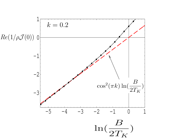
Figure 4: Showing logarithmic dependence of $Re[1/{\cal J}(0)]$ on magnetic field at zero temperature, calculated numerically for the case $k=0.2$. The magnetic field provides the cut-off to the logarithmic scaling. For details of how the magnetic field was introduced, see section VI. Dashed line is the the curve $y=\cos^{2}(\pi k)ln(\frac{B}{2T_{K}})$.

At low temperatures ${\cal J}$ scales to zero with logarithmic slowness. If we look at the the conduction electron self-energy as given by (20), we see that the leading singular frequency dependence is given by the $kn_{b}{\cal J}(\omega)$ term, so that at low frequencies,

$$\Sigma(\omega)=-\frac{k(n_{b}+\theta(\nu))\sec^{2}(\pi k)}{\rho\left[\ln\left(\frac{T_{K}}{|\omega|}\right)+i\pi[n_{b}+\theta(\omega)]\right]}-\frac{\tan(\pi k)}{\pi\rho}=-\frac{\tan(\delta(\omega))}{\pi\rho}$$ (28)

where

$$\delta_{c}(\omega)\sim\pi k\left[1+\frac{[n_{b}+\theta(\omega)]}{\ln(T_{K}/|\omega|)}\right]+O\left(\frac{1}{\ln^{2}(T_{K}/|\omega|)}\right).$$ (29)

This singular energy dependence of the conduction electron phase shift is a consequence of coupling between the degenerate manifold of the partially screened moment and the conduction sea. Although the scattering of conduction electrons is elastic at low energies, the singular frequency dependence displayed here sets this system apart from a conventional Landau Fermi liquid (where the phase shift depends linearly on energy). Indeed, if we use $\Sigma(\omega)$ to define a frequency dependent wave-function renormalization constant, we find that this quantity diverges as $Z=\frac{1}{1-\Sigma^{\prime}(\omega)}\sim\frac{1}{\omega\log(T_{K}/\omega)}$, so that there are no well-defined quasiparticles associated with the Kondo scattering. This is the meaning of the term “singular” Fermi liquid.

The singular energy dependence of the scattering is also reflected in the shape of the Abrikosov Suhl resonance, given by the imaginary part of the electron t-matrix

$$Im[t(\omega)]=Im\left[\frac{\Sigma(\omega)}{1-g_{0}(\omega)\Sigma(\omega)}\right]\sim\frac{1}{\pi\rho}\left[\sin^{2}(\pi k)+\frac{\pi k[n_{b}+\theta(\omega)]\sin(2\pi k)}{\ln(T_{K}/|\omega|)}\right].$$ (30)

These basic features are each borne out in the detailed numerical solution of the integral mean-field equations of the large $N$ limit. Fig. 5. shows the results of this numerical calculation, showing the spectral function of the t-matrix and the dependence of the phase shift on the number of flavors.

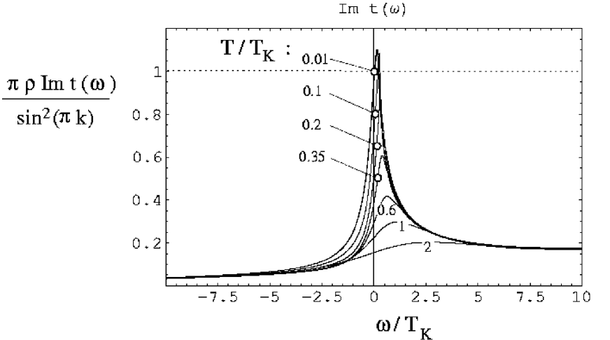
Figure 5: Showing the frequency dependence of the t-matrix, normalized with respect to zero temperature value at Fermi energy. In this numerical calculation, $k=K/N=0.45$, $n_{b}=2S/N=0.2$. Numerical labels give temperature $T/T_{K}$.

This singular energy dependence of the t-matrix also manifests itself in the temperature dependent resistivity, given by

$$\frac{\rho(T)}{\rho_{U}}=n_{i}\pi\rho\int d\omega\left(-\frac{\partial f}{\partial\omega}\right)Imt(\omega)$$ (31)

where $\rho_{U}=\left(\frac{ne^{2}}{m}\frac{2}{\pi\rho}\right)^{-1}$ is the unitary resistivity as shown in Fig. 6.

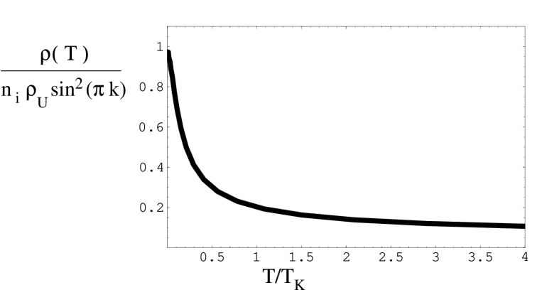
Figure 6: Showing the temperature dependence of the single impurity resistance $\rho(T)$, per unit concentration of impurity. For this plot, $k=K/N=0.45$, $n_{b}=2S/N=0.2$.

V Phase shift and the screening of the moment

To reveal the screening of the local moment, we need to compute the first correction to the constraint equation. To satisfy the constraint we must differentiate the Free energy (12) w.r.t $\lambda$. This yields

$$2SK = KNn_{b}+\delta{\cal N}_{b}$$ (32)

$$\delta{\cal N}_{b} = -T^{2}{K}\sum_{i\nu_{n},i\omega_{r}}\frac{1}{(i\nu_{n}-\lambda)^{2}}g(i\nu_{n}+i\omega_{r}){\cal J}(i\omega_{r}).$$ (33)

The first term in this sum determines the number of bosons that condense into the unscreened magnetic moment. The second term $\delta{\cal N}_{b}$ is the total number of bosons bound into the Kondo singlet in the ground-state.

At zero temperature we can replace the discrete Matsubara sums by a continuous integral as follows,

$$T\sum_{i\nu_{n}}\longrightarrow\int_{-i\infty}^{{i\infty}}\frac{d\nu}{2\pi i},\qquad T\sum_{i\omega_{r}}\longrightarrow\int_{-i\infty}^{{i\infty}}\frac{d\omega}{2\pi i},$$

so that the number of bound-bosons becomes

$$\delta{\cal N}_{b}=K\int\frac{d\omega}{(2\pi i)}\int\frac{d\nu}{(2\pi i)}g(\nu+\omega)\frac{\partial}{d\nu}\left(\frac{1}{\nu-\lambda}\right){\cal J}(\omega),$$ (34)

where we have replaced $\frac{1}{(\nu-\lambda)^{2}}\rightarrow-\frac{\partial}{d\nu}\left(\frac{1}{(\nu-\lambda)}\right)$. Next we can integrate the internal integral by parts

$$\delta{\cal N}_{b}=-K\int\frac{d\omega}{(2\pi i)}\int\frac{d\nu}{(2\pi i)}\frac{\partial}{d\nu}\left(g(\nu+\omega)\right)\frac{1}{\nu-\lambda}{\cal J}(\omega),$$ (35)

and then replace $\frac{\partial}{d\nu}\rightarrow\frac{\partial}{d\omega}$ to obtain

$$\delta{\cal N}_{b}=K\int\frac{d\omega}{(2\pi i)}\frac{\partial}{d\omega}\overbrace{\left(-\int\frac{d\nu}{(2\pi i)}g(\nu+\omega)\frac{1}{\nu-\lambda}\right)}^{{\Pi(\omega)}}{\cal J}(\omega),$$ (36)

We can now identify the term inside the central brackets as the self-energy $\Pi(\omega)$, which enables us to compactly rewrite the integral as

$$\delta{\cal N}_{b} = K\int\frac{d\omega}{(2\pi i)}\frac{\partial}{d\omega}\left(\Pi(\omega)\right){\cal J}(\omega)$$ (37)

$$= -K\int\frac{d\omega}{(2\pi i)}\frac{\partial}{d\omega}\ln\left[-{\cal J}^{-1}(\omega)\right]$$ (38)

$$= -\frac{K}{\pi}\left[\delta_{\phi}(0)-\delta_{\phi}(-\infty)\right]=-\frac{K}{\pi}\delta_{\phi}$$ (39)

where

$$\delta_{\phi}(\omega)={\rm Im}\ln\left[\frac{1}{J}-\Pi(\omega-i\delta)\right].$$

so that

$$K2S=\overbrace{NKn_{b}}^{2KS^{*}}-\overbrace{\frac{K}{\pi}\delta_{\phi}}^{{\delta n_{b}}}.$$

Now the argument inside the logarithm that determines $\delta_{\phi}$ is the inverse of the running coupling constant,

$$\frac{1}{{\cal J}(\omega)}=\frac{1}{J}-\Pi(\omega-i\delta).$$

In the underscreened Kondo model, the residual coupling between the partially screened local moment and the conduction electrons becomes ferromagnetic at low temperatures, scaling logarithmically to zero. This means that $\frac{1}{{\cal J}(\omega-i\delta)}\sim-\rho^{-1}\ln(T_{K}/\omega)-i\delta$ at low energies, which implies that $\delta_{\phi}=-\pi$. This in turn, implies that the number of bound-bosons is $\delta{\cal N}_{b}=K$. As a consequence the number of unpaired bosons is reduced by $K$ in the ground-state, and if we define $S^{*}=\frac{N}{2}n_{b}$, the effective spin of each flavor will be

$$S^{*}=S-\frac{1}{2}.$$

We can also relate the number of bound bosons to the conduction electron phase shift $\delta_{c}$, in a parallel fashion, as follows:

$$\delta{\cal N}_{b} = K\int\frac{d\omega}{(2\pi i)}\frac{\partial}{d\omega}\overbrace{\left(\int\frac{d\nu}{2\pi i}{\cal J}(\omega-\nu)\frac{1}{\nu-\lambda}\right)}^{-\Sigma(\omega)}g(\omega)$$ (40)

$$= -N\int\frac{d\omega}{(2\pi i)}\frac{\partial\Sigma(\omega)}{d\omega}{g}(\omega)$$ (41)

$$= N\int\frac{d\omega}{(2\pi i)}\frac{\partial}{d\omega}\ln\left[g_{o}^{-1}-\Sigma(\omega)\right]$$ (42)

$$= \frac{N}{\pi}\left[\delta_{c}(0)-\delta_{c}(-\infty)\right]=\frac{N}{\pi}\delta_{c}.$$ (43)

In deriving the third line of this expression, we have taken the large band-width limit, enabling all frequency dependence of the conduction green function $g_{o}=-i\pi\rho{\rm sign}(\omega_{n})$ to be be ignored. The conduction electron phase shift is given by

$$\delta_{c}(\omega)={\rm Im}\ln\left[1-g_{0}(\omega-i\delta)\Sigma(\omega-i\delta)\right].$$ (44)

By comparing the two expressions (34 ) and (40 ) for $\delta{\cal N}_{b}$, we are able to confirm that the conduction electron phase shift is given by

$$\delta_{c}=\pi\left(\frac{\delta{\cal N}_{b}}{N}\right)=\pi k.$$

Notice that along the way we have proven that

$$N\left(\frac{\delta_{c}}{\pi}\right)+K\left(\frac{\delta_{\phi}}{\pi}\right)=0$$ (45)

Although we have proven this strictly in the large N limit, this result is a Ward Identity that is expected to hold for all $N$, a result which relies solely on Fermion number conservation (see Appendix A). This result is in effect, a statement of famous the “Anderson-Clogston compensation theorem” - that the total number of bound fermions bound by the Kondo effect in the infinite band-width limit, is zeroclogston61 .

VI Zero temperature Magnetization

In order to examine the effect of a magnet field in the large $N$ limit we need to be careful about our definition of the magnetization. We shall suppose that the magnetic field couples preferentially to the “up” spin (s) of each flavor, i.e. that the magnetization takes the form

$$\hat{M}=g_{N}(\hat{n}_{b\uparrow\mu}-\hat{n}_{b\uparrow\mu}|_{B=0})$$

There are various ways in which we can now definite $\hat{n}_{b\uparrow\mu}$. One way to do this, is to define the “up” states as the first $K$ spin components, i.e

$$\hat{M}^{(1)}=\frac{N}{2(N-K)}\left[\sum_{\mu,\sigma=1}^{K}\hat{n}_{b\sigma\mu}-\frac{2SK^{2}}{N}\right]$$

Here, value of $g_{N}$ is chosen so that at full polarization, $M=SK$. With this definition, the first $K$ spin channels of the conduction electron are “up” electrons and the remaining $N-K$ spin channels are “down”. When we add $\hat{M}^{(1)}$ to the corresponding expression for the conduction electrons, we form a conserved quantity, so that we shall call $M^{(1)}$ the “conserved magnetization”. By imposing the constraint, $\sum_{\sigma\mu}n_{b\sigma\mu}=2SK$, the conserved magnetization can be rewritten as

$$\hat{M}^{(1)}=\frac{1}{2}\left[2SK-\frac{N}{N-K}n_{b\downarrow}\right]$$

where $n_{b\downarrow}=2SK-n_{b\uparrow}=\sum_{\mu=1}^{K}\sum_{\sigma>K}n_{b\sigma\mu}$. Now unfortunately, if we couple the magnetic field up to $M^{(1)}$, then we do not completely remove the spin degeneracy of the ground-state. For this purpose, we need a more restrictive definition of $n_{b\uparrow}$, and we shall choose “up” to mean the spin component where $\mu=\sigma$, i.e

$$n_{b\uparrow}\equiv\sum_{\mu=1}^{K}\sum_{\sigma=1}^{N}n_{b\sigma\mu}\delta_{\mu\sigma}=\sum_{\mu=1}^{K}n_{b\mu\mu}.$$

With this definition, by imposing the constraint, $\sum_{\sigma\mu}n_{b\sigma\mu}=2SK$, we obtain

$$\hat{M}=KS-\frac{1}{2}\sum_{\sigma\neq a}n_{b\sigma a}$$

We shall use this definition as our method for coupling the magnetic field to the spin, so that $M=-\delta F/\delta H$ is the true “thermodynamic” magnetization. In the case where $K=1$, the thermodynamic and conserved magnetizations correspond exactly. However, the need to break the flavor or replica symmetry at finite $K$ unfortunately forces us to delineate between these two forms. However, we shall see shortly that $\langle M^{(1)}\rangle$ and $\langle M\rangle$ have almost identical expectation values, and that the conserved magnetization has a far more convenient expression in terms of the scattering phase shift. The coupling to a magnetic field then gives the Hamiltonian

$$H_{B}=-B\hat{M}=-BKS+\frac{B}{2}\sum_{\sigma\neq a}n_{b\sigma a}.$$ (46)

Now in the large $N$ limit at low temperatures in a field, the “up” bosons condense. This allows us to carry out the Kondo version of spin-wave theory. Formally, we condense the “up” bosons and integrate over their phase fluctuations to exactly impose the constraint. The resulting Holstein Primakoff transformation is obtained by replacing

$$\hat{b}_{\sigma a}\rightarrow\left\{\begin{array}[]{cr}\sqrt{2S-n_{ba}}&(\sigma=a),\cr b_{\sigma a}&(\sigma\neq a)\end{array}\right.$$ (47)

where $n_{ba}=\sum_{\sigma\neq a}b^{\dagger}_{\sigma a}b_{\sigma a}$. In this process, the $\sigma=a$ or “up” components of the boson fields have been eliminated. In a field, the amount of fluctuations $n_{ba}\sim O(1)$, so that as in spin-wave theory, to leading order, we can drop the $n_{ba}$ inside the square-root. With this understanding, inside the interaction, we must now make the replacement

$$\sum_{\beta}\psi^{\dagger}_{\beta}b_{\beta a}\rightarrow\psi^{\dagger}_{a}\sqrt{2S}+\sum_{\beta^{\prime}\neq a}\psi^{\dagger}_{\beta^{\prime}}b_{\beta^{\prime}a}$$

so that the Hamiltonian in a field now becomes

$$H = \sum_{k\alpha}\epsilon_{k}c^{\dagger}_{k\alpha}c_{k\alpha}+H_{I}+H_{B}$$ (48)

$$H_{I} = \frac{1}{\sqrt{N}}\left\{\sum_{a=1}^{K}\left(\psi^{\dagger}_{a}\sqrt{2S}+\sum_{\beta^{\prime}\neq a}\psi^{\dagger}_{\beta^{\prime}}b_{\beta^{\prime}a}\right)\phi_{a}+H.c\right\}-\sum_{a=1}^{K}\frac{\bar{\phi}_{a}\phi_{a}}{J}$$ (49)

$$H_{B} = B\left(\frac{1}{2}\sum_{a=1}^{K}n_{ba}-KS\right)$$ (50)

The effective action in a field now becomes

$$S = \int_{0}^{\beta}d\tau\left[\sum_{k,\sigma}c^{\dagger}_{k\sigma}\left(\partial_{\tau}+\epsilon_{k}\right)c_{k\sigma}-\frac{1}{J}\bar{\phi}_{\mu}\phi_{\mu}-SK(2\lambda+B)\right]+S_{I}+S_{mix}$$ (51)

$$S_{I} = -\frac{1}{N}\sum_{a=1}^{K}\sum_{\sigma\neq a}\int_{0}^{\beta}d\tau d\tau^{\prime}\psi^{\dagger}_{\sigma}(\tau)\psi_{\sigma}(\tau^{\prime})D_{\sigma}(\tau-\tau^{\prime})\bar{\phi}_{a}(\tau^{\prime})\phi_{a}(\tau)$$ (52)

$$S_{mix} = \sqrt{\frac{2S}{N}}\sum_{a=1}^{K}\int_{0}^{\beta}d\tau\left[\psi(\tau)^{\dagger}_{a}\phi(\tau)_{a}+\bar{\phi}_{a}(\tau)\psi_{a}(\tau)\right]$$ (53)

where $D_{\sigma}(i\nu_{n})=\frac{1}{i\nu_{n}-(B/2)}$. The interaction term $S_{I}$ can be split up into a term with no restrictions on the spin flavor summations, plus a term ${\cal R}$ that can be neglected in the large $N$ limit:

$$S_{I} = -\frac{1}{N}\sum_{a=1}^{K}\sum_{\sigma=1}^{N}\int_{0}^{\beta}d\tau d\tau^{\prime}\psi^{\dagger}_{\sigma}(\tau)\psi_{\sigma}(\tau^{\prime})D_{\sigma}(\tau-\tau^{\prime})\bar{\phi}_{a}(\tau^{\prime})\phi_{a}(\tau)+{\cal R}$$ (54)

$$\cal R = \frac{1}{N}\sum_{a=1}^{K}\int_{0}^{\beta}d\tau d\tau^{\prime}\psi^{\dagger}_{a}(\tau)\psi_{a}(\tau^{\prime})D_{\sigma}(\tau-\tau^{\prime})\bar{\phi}_{a}(\tau^{\prime})\phi_{a}(\tau).$$ (55)

If we carry out a Hubbard Stratonovich decoupling on the first term, we now have:

$$S = \int_{0}^{\beta}d\tau d\tau^{\prime}{\cal L}(\tau,\tau^{\prime})-\beta SKB$$ (56)

$${\cal L} = \sum_{\sigma>K}\psi^{\dagger}_{\sigma}\left[-g_{0}^{-1}+\Sigma\right]\psi_{\sigma}+\sum_{a=1}^{K}\left(\psi^{\dagger}_{a},\bar{\phi}_{a}\right)\left[\begin{matrix}-g_{0}^{-1}+\Sigma&\sqrt{\tilde{n}_{b}}\cr\sqrt{\tilde{n}_{b}}&-J^{-1}+\Pi\end{matrix}\right]\left(\begin{matrix}\psi_{a}\cr\phi_{a}\end{matrix}\right)$$ (57)

$$+ N\Pi(\tau-\tau^{\prime})\frac{1}{D_{0}(\tau-\tau^{\prime})}\Sigma(\tau^{\prime}-\tau)$$ (58)

where $\tilde{n}_{b}=2S/N$ Taking the saddle point values for $\Pi$ and $\Sigma$, and then integrating out the fermions, the mean-field free energy in a field is then

$$\frac{F}{NT} = -(1-k){\rm Tr}\ln\left[-g_{o}^{-1}+\Sigma\right]-k{\rm Tr}\ln\left[\begin{matrix}-g_{0}^{-1}+\Sigma&\sqrt{\tilde{n}_{b}}\cr\sqrt{\tilde{n}_{b}}&-J^{-1}+\Pi\end{matrix}\right]$$ (59)

$$+ N\int d\tau d\tau^{\prime}\Pi(\tau^{\prime},\tau)\frac{1}{D_{0}(\tau-\tau^{\prime})}\Sigma(\tau,\tau^{\prime})-SKB.$$ (60)

When we impose the saddle-point condition on $\Sigma$ and $\Pi$, decomposition, we must be careful to delineate between the propagators of “up” and “down” electrons. The mean-field equations are then

$$\Sigma(\tau-\tau^{\prime}) = -kD(\tau-\tau^{\prime}){\cal J}(\tau-\tau^{\prime})$$ (61)

$$\Pi(\tau-\tau^{\prime}) = -D(\tau^{\prime}-\tau)[kg_{\uparrow}(\tau-\tau^{\prime})+(1-k)g_{\downarrow}].$$ (62)

The mixing terms between the “up” electrons and the “phi” fields mean that we must now modify the propagators as follows:

$$g_{\downarrow}(\omega) = \frac{1}{g_{0}^{-1}(\omega)-\Sigma_{\downarrow}(\omega)}$$ (63)

$$g_{\uparrow}(\omega) = \frac{1}{g_{0}^{-1}(\omega)-\Sigma_{\uparrow}(\omega)}.$$ (64)

Here

$$\Sigma_{\downarrow}(\omega) = \Sigma(\omega)$$ (65)

$$\Sigma_{\uparrow}(\omega) = \Sigma(\omega)+\tilde{n}_{b}\left(J^{-1}-\Pi(\omega)\right)^{-1}$$ (66)

and

$${\cal J}(\omega)=\frac{1}{J^{-1}-\Pi(\omega)-\tilde{n_{b}}g_{\downarrow}(\omega)}$$ (67)

where $\tilde{n}_{b}=2S/N$.

If we convert the integral equations to Matsubara summations, we obtain

$$\Sigma(i\omega_{n}) = -k\sum_{r}\frac{1}{i\nu_{r}-(B/2)}{\cal J}(i\omega_{n}-i\nu_{r})$$ (68)

$$\Pi(i\omega_{n}) = -\sum_{r}\frac{1}{i\nu_{r}-(B/2)}\left(kg_{\uparrow}(i\omega_{n}+i\nu_{r})+(1-k)g_{\downarrow}(i\omega_{n}+i\nu_{r})\right)$$ (69)

Carrying out the Matsubara summations, we then obtain

$$\Sigma(z) = k\int\frac{dy}{\pi}\frac{1-f(y)}{z-y-(B/2)}Im{\cal J}(y-i\delta)$$ (70)

$$\Pi(z) = \int\frac{dy}{\pi}\frac{f(y)}{z-y+(B/2)}Im\left[kg_{\uparrow}(y-i\delta)+(1-k)g_{\downarrow}(y-i\delta)\right].$$ (71)

From the solutions of these equations, we can compute the field dependent propagators and free energy. We can define the following scattering phase shifts associated with the conduction electrons and $\phi$ fermion:

$$\delta_{\phi}(B) = {\rm Im}\left[\phantom{\int}\hskip-11.38092pt\ln\bigl{(}1-J[\Pi(z)+\tilde{n}_{b}g_{\downarrow}(z)]\bigr{)}\right]_{z=0-i\delta}.$$ (72)

$$\delta_{c\sigma}(B) = {\rm Im}\left[\phantom{\int}\hskip-11.38092pt\ln\bigl{(}1-g_{0}\Sigma_{\sigma}(z)\bigr{)}\right]_{z=0-i\delta},\qquad\qquad(\sigma=\uparrow,\ \downarrow)$$ (74)

These phase shifts at finite field are actually related by Ward identities (see appendix B), and obey the following relationships at all fields:

$$K\delta_{\phi}+N\delta_{\downarrow} = 0$$ (75)

$$K\delta_{\uparrow}+(N-K)\delta_{\downarrow} = K\pi$$ (76)

The differentiation of the Free energy w.r.t. field is identical to the differentiation w.r.t. $\lambda$ carried out in the previous section. The magnetization is given by

$$M = SK-\frac{{\delta{\cal N}_{b}}}{2}$$ (77)

$$\delta{\cal N}_{b} = -T^{2}{K}\sum_{i\nu_{n},i\omega_{r}}\frac{1}{(i\nu_{n}-B/2)^{2}}\tilde{g}(i\nu_{n}+i\omega_{r}){\cal J}(i\omega_{r}),$$ (78)

where $\tilde{g}=kg_{\uparrow}+(1-k)g_{\downarrow}$. If, instead of using the thermodynamic magnetization, we use the conserved magnetization $M^{(1)}$, then we find that

$$M^{(1)} = SK-\frac{{\delta\tilde{{\cal N}}_{b}}}{2}$$ (79)

$$\delta\tilde{{\cal N}}_{b} = -T^{2}{K}\sum_{i\nu_{n},i\omega_{r}}\frac{1}{(i\nu_{n}-B/2)^{2}}g_{\downarrow}(i\nu_{n}+i\omega_{r}){\cal J}(i\omega_{r}),$$ (80)

The difference between the two expressions results from the slight energies. The advantage of the second quantity, is that by being related to a conserved quantity, it is related to the scattering phase shifts. Using exactly the same methods we relate $\delta\tilde{{\cal N}}_{b}$ to the $\phi$ and conduction electron phase shifts, as before, to obtain

$$M^{(1)} = KS+\frac{K}{2}\frac{\delta_{\phi}(B)}{\pi}$$ (81)

$$= KS-\frac{N}{2}\frac{\delta_{\downarrow}(B)}{\pi}$$ (82)

$$= K(S-\frac{1}{2})+\frac{K}{2}\frac{\delta_{\uparrow}(B)-\delta_{\downarrow}(B)}{\pi}$$ (83)

where we have used the phase-shift identities (75) given above.

We have solved equations (63, 65, 70) at zero temperature, finite field $B$ by numerical iteration, using a Fast Fourier transfer routine to carry out the convolutions. Fig. 7 shows the field dependence of the coupling constant $g(B)=Re[{\cal J}(\omega)|_{\omega=0}$, showing the change in sign of the coupling constant as the system goes from weak coupling at high fields to strong coupling at low fields.

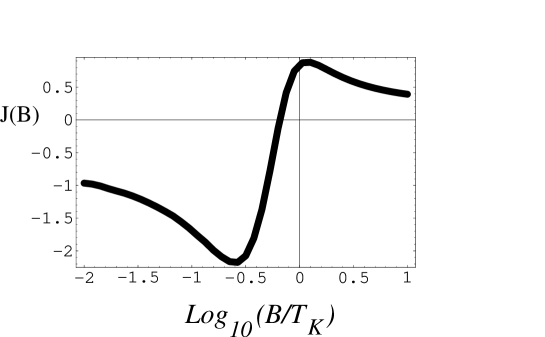
Figure 7: Dependence of the Kondo coupling constant on field for $k=0.45$.

Fig. 8 shows the field dependence of the “up” and “down” phase shifts. The results obtained by our large $N$ method are strikingly similar to results recently obtained by numerical renormalization group and the Bethe ansatzborda . Fig. 9 shows the field dependent reduction in the magnetization $\Delta M=-K\delta_{\phi}(B)/\pi$.

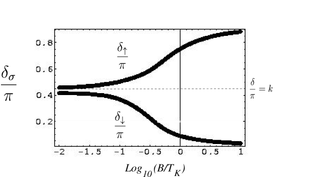
Figure 8: Field dependence of the “up” and “down” phase shifts for $k=0.45$.

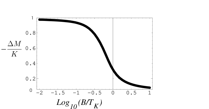
Figure 9: Field dependence of the magnetization reduction $\Delta M/K=\delta_{\phi}/\pi$ for $k=0.45$

VII Discussion

Our method gives a controlled treatment of the underscreened Kondo model, and using the method of replicas, we have been able to develop a treatment of the Kondo effect which correctly reproduces the finite phase shift $\delta=\pi K/N$ produced by the scattering resonance.

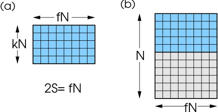
Figure 10: (a) Rectangular Young Tableau which will self-assemble in strong-coupling ground-state (b) of color-flavor-spin model in the case where $F=2S$.

What are the prospects for going further?

The first question of interest, is whether this approach can be used to describe the fully quenched Fermi liquid? An adhoc way to attempt to access the Fermi liquid, is to seek solutions where

$${\cal N}_{b}=K=2KSn_{b}(\lambda)+N\frac{\langle\delta_{c}\rangle}{\pi}$$

The presence of the additional term in the constraint then raises the value of $\lambda$, so that in the ground-state $\lambda\neq 0$, and hence $n_{b}\rightarrow 0$, producing a fully quenched ground-state. The obvious drawback with this approach, is that by pushing the problem to this limit, we are exploring a limit where the occupancy of each boson spin/flavor state is of order $O(1/N)$, which lies outside the strict region of validity for the large $N$ expansion.

A more encouraging approach to the problem may lie in trying to unify the boson replica approach used here, with the multi-channel approach developed by Parcollet and Georges (PG). The PG approach introduces F flavors of conduction electron, considering an interaction of the form

$$H_{I} = \frac{J}{N}\sum_{\gamma=1}^{F}\sum_{\alpha\beta}(\psi^{\dagger}_{\beta\gamma}b_{\beta})(b^{\dagger}_{\alpha}\psi_{\alpha\gamma})$$ (84)

This approach leads to a scattering phase shift $\delta=\pi/N$ which vanishes in the large $N$ limit, however, it has the virtues that for $F=2S$ it does describe a fully quenched Fermi liquid, and moreover, the method can, in the lattice, be neatly combined with the Arovas-Auerbacharovas treatment of antiferromagnetism, using a SP (2N) description of the RKKY interactions readsachdev91 ; zarand .

Is it possible to extend this model, introducing both conduction flavor and boson color at the same time? This suggests the following color-flavor-spin (CFS) model

$$H_{I} = \frac{J}{N}\sum_{\alpha,\beta,\gamma,\mu}(\psi^{\dagger}_{\beta\gamma}b_{\beta\mu})(b^{\dagger}_{\alpha\mu}\psi_{\alpha\gamma})\qquad\qquad(\gamma\in[1,F],\ \mu\in[1,K])$$ (85)

where we choose $2S=F=fN$, and $K=kN$ in the large $N$ limit. The strong-coupling solution to this model involves the formation of a singlet between a rectangular representation of the Bosons, and the $F$ channels of conduction electron, as shown in Fig. 10. In the ground-state, we expect the bosons to self-assemble into this strong-coupling representation.

To develop a large $N$ expansion of the CFS model, we might consider writing down the connected skeleton graphs that enter into the Luttinger-Wardluttingerward functional $Y[G,{\cal J},D]$. The two leading diagrams in $Y$ take the form shown in Fig. 11.

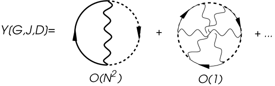
Figure 11: Two leading order skeleton diagrams for the Luttinger Ward functional of the CFS model.

There is one loop for each quantum number in each of the above diagrams, but because the second diagram involves more vertices, it is smaller by a factor of $O(1/N^{2})$. $Y$ can be used to generate the self-energies for a conserving approximation, via the relationships:

$$-\frac{\delta Y}{\delta G(i\omega_{n})} = NF\Sigma(i\omega_{n}),$$ (86)

$$-\frac{\delta Y}{\delta{\cal J}(i\omega_{n})} = KF\Pi(i\omega_{n}),$$ (87)

$$\frac{\delta Y}{\delta D(i\nu_{n})} = NK\Sigma_{b}(i\nu_{n}),$$ (88)

where the pre-factors arise because of the sum over spin, flavor and channel that arises inside $Y$. The first term in this series can be used to generate the diagrams that interpolate between the PG and the replica approach. This term in the skeleton expansion of the Free energy is of order $O(N^{2})$ in an approach that involves color, flavor and spin. Since next skeleton diagram is of order $O(1)$, so that at first sight, we may neglect all higher order diagrams.

However, it turns out that the development of a strict large $N$ expansion encounters a technical difficulty with the profusion of higher order planar diagrams. Similar difficulties have been encountered in the large $N$ treatment of quantum chromodynamics (QCD). To see this, it is useful to relabel the conduction, boson and $\phi$ propagators as two parallel lines, carrying the respective quantum numbers of spin, color and flavor, as follows

With this notation, we see that introduction of the additional flavor quantum number, means that the interaction vertex between bosons is enhanced by the sum over virtual flavor fluctuations, from from a $O(1/N^{2})$ term in the current theories, to a $O(1/N)$ vertex as shown below.

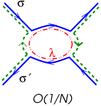
Figure 12: Magnetic vertex. The additional flavor index enhances this vertex by a factor of $N$.

If we now look at the boson self-energy diagram generated by this vertex,

$\raisebox{-25.29494pt}[0.0pt][0.0pt]{\psfig{width=108.405pt}}=O(1/N^{2}\times N^{2})=O(1)$

we see it is of order $O(1)$. Furthermore, when we close the external legs on this diagram to

create a skeleton graph,

$\raisebox{-36.135pt}[0.0pt][0.0pt]{\psfig{width=180.67499pt}}\qquad=\qquad O(N^{6}/N^{4})=O(N^{2})$

we see that this graph (which contains six internal quantum number loops, ) is of order $O(N^{2})$- the same order as the leading graph. Unfortunately, as in QCD, this is just the beginning of an entire profusion of higher order “planar diagrams” which are all of the same order in the large $N$ expansion.

Despite this difficulty, it may be that the leading order $O(N^{2})$ diagram shown in Fig. 9 is already sufficient to generate a good conserving mean-field theory for the fully quenched Kondo model. We do not yet know how the neglect of the higher order planar diagrams affects the results, but it is tempting to speculate that these diagrams are irrelevant in the Fermi liquid, or magnetic ground-state, since the flavor and color quantum numbers become massive when the Kondo singlet forms, or when there is an applied magnetic field. In this case, the higher order diagrams may only renormalize the leading order term in the skeleton graph expansion of the Free energy. These considerations lead us to suggest that the leading order skeleton free energy diagram for the color-flavor-spin model may provide the key to a successful mean-field theory that spans the magnetic quantum critical point.

One of the interesting final questions that deserves discussion, concerns the physical significance of the additional quantum numbers that we have introduced. The color-flavor-spin large $N$ approach is basically approximating the single box of the Young Tableau representing a spin $1/2$ by a rectangular Young tableau. What is the meaning of the intensive variables $f=F/N$ and $k=K/N$ that appear in the PG and the current approach? One fascinating possibility, is that quantum numbers associated with these degrees of freedom describe the internal quantum numbers of the composite quasiparticle in the heavy electron state. In the Fermi liquid, we expect these quantum numbers to be inert, but at the quantum critical point, these quantum numbers become unconfined. These issues will be followed in forthcoming work.

This research is supported by the National Science Foundation grant NSF DMR 0312495. We should particularly like to thank Anirvan Sengupta for discussions concerning the matrix aspects of the CFS model, and the profusion of planar diagrams. Shortly after submitting this paper to the archive, we became aware of a closely related fermionic “replica” approach by S. Florens, which we have referenced in this revised draft.florens Discussions with N. Andrei, G. Kotliar, P. Mehta, G. Zarand and L. Borda are gratefully acknowledged.

VIII Appendix A

In this appendix, we derive the Ward Identity

$$N\left(\frac{\delta_{c}}{\pi}\right)+K\left(\frac{\delta_{\phi}}{\pi}\right)=0$$

and relate it to the Anderson-Clogston compensation theorem. According to this theorem clogston61 , the net polarization of the conduction sea by a localized impurity is zero, in the limit of a broad band. A localized resonant scattering center induces Friedel oscillations in charge density of the medium, and tends to reduce the charge density in the immediate vicinity of the impurity. The compensation guarantees that this local depression in charge density is compensated by an enhancement at greater distances.

To understand this compensation effect, we need to examine the conduction electron Greens function, which is given by

$$G_{\bf{k},\bf{k}^{\prime}}(i\omega_{n})=\frac{\delta_{\bf{k},\bf{k}^{\prime}}}{i\omega_{n}-\epsilon_{\bf{k}}}+\frac{1}{i\omega_{n}-\epsilon_{\bf{k}}}t(i\omega_{n})\frac{1}{i\omega_{n}-\epsilon_{\bf{k}^{\prime}}}$$

where $t(i\omega_{n})$ is the t-matrix of the impurity. The second term in this expression induces the Friedel oscillations in charge density, which are given by

$$\Delta\rho({\bf{x}})=NT\sum_{{\bf{k}},{\bf{k}}^{\prime},i\omega_{n}}\frac{1}{i\omega_{n}-\epsilon_{\bf{k}}}t(i\omega_{n})\frac{1}{i\omega_{n}-\epsilon_{\bf{k}^{\prime}}}e^{i(\bf{k}-\bf{k}^{\prime})\cdot\bf{x}}e^{i\omega_{n}0^{+}}$$

For example, the change in density at the impurity is given by

$$\Delta\rho({\bf{0}})=-N(\pi\rho)^{2}\int_{-\infty}^{\infty}\frac{d\omega}{\pi}f(\omega){\rm Im}t(\omega-i\delta)<0$$

( where we have carried out the momentum sum, replacing $\sum_{{\bf{k}}}(i\omega_{n}-\epsilon_{{\bf{k}}})\rightarrow-i\pi\rho{\rm sgn}(n)$), corresponding to a reduction in the electron density. By contrast, the total change in density,

$$\Delta Q=\int d^{3}x\Delta\rho({\bf{x}})=NT\sum_{{\bf{k}},i\omega_{n}}\frac{1}{(i\omega_{n}-\epsilon_{{\bf{k}}})^{2}}t(i\omega_{n})e^{i\omega_{n}0^{+}}$$ (89)

Assuming that the width of the resonance is much narrower than the bandwidth $D$, we can replace

$$\sum_{{\bf{k}}}\frac{1}{(i\omega_{n}-\epsilon_{{\bf{k}}})^{2}}\rightarrow\rho\int_{-D}^{D}d\epsilon\frac{1}{(i\omega_{n}-\epsilon)^{2}}=\frac{2\rho}{D}+O(\frac{\omega_{n}\rho}{D^{2}})$$

so that

$$\Delta Q = \frac{2\rho}{D}T\sum_{i\omega_{n}}t(i\omega_{n})e^{i\omega_{n}0^{+}}=\frac{\Gamma}{\pi D}\sim 0$$ (90)

where

$$\Gamma=2\pi\rho\int_{-\infty}^{\infty}\frac{d\omega}{\pi}f(\omega){\rm Im}t(\omega-i\delta)$$

is a measure of the width of the resonance. Thus the total polarization of the conduction band is of order $\Gamma/D<<1$, which is negligible in the limit of infinite bandwidth.

Now we shall relate $\Delta Q$ to the scattering phase shifts. To do this, we appeal to the Luttinger-Ward functional $Y[G,{\cal J}]$for this problem, represented by a sum over all skeleton closed loop diagram contributions. The differential of this functional with respect to the Greens functions generates the corresponding self-energies:

$$-\frac{\delta Y}{\delta g_{\sigma}(i\omega_{n})} = \Sigma_{\sigma}(i\omega_{n}),$$ (91)

$$-\frac{\delta Y}{\delta{\cal J}_{\mu}(i\omega_{n})} = \Pi_{\mu}(i\omega_{n}),$$ (92)

where we have explicitly displayed the spin and flavor indices. Now the conservation of charge guarantees that each of these can be decomposed into one or more closed fermion lines. In the low temperature limit, the Matsubara sums along these lines may be replaced by continuous integrals along the imaginary axis,

$$T\sum_{i\omega_{n}}\dots\rightarrow\int\frac{dz}{2\pi i}\dots$$

Now if, at zero temperature, the frequency running along each such loop is incremented by a small amount $z\rightarrow z+i\delta\omega$, $Y$ is unchanged, because the the shift in $z$ can be absorbed by a simple change of variable. We deduce that at $T=0$, in the absence of a field,

$$\delta Y = i\delta\omega\int\frac{d\omega}{2\pi i}\left[\sum_{\sigma=1}^{N}\frac{\delta Y}{\delta g_{\sigma}(\omega)}\frac{dg_{\sigma}}{d\omega}+\sum_{\mu=1}^{K}\frac{\delta Y}{\delta{\cal J}_{\mu}(\omega)}\frac{d{\cal J}_{\mu}}{d\omega}\right]$$ (93)

$$= -i\delta\omega\int\frac{d\omega}{2\pi i}\left(N\Sigma(\omega)\frac{dg}{d\omega}+K\Pi(\omega)\frac{d{\cal J}}{d\omega}\right)=0$$ (94)

Integrating this result by parts, we obtain

$$0=\int\frac{d\omega}{2\pi i}\left(Ng(\omega)\frac{d\Sigma}{d\omega}+K{\cal J}(\omega)\frac{d\Pi}{d\omega}\right)$$ (95)

This valuable result is a consequence of fermion, or charge conservation.

Now the total change in the charge of the system is given by

$$\Delta Q = NT\sum_{i\omega_{n}}\left[g(i\omega_{n})-g_{0}(i\omega_{n})\right]e^{i\omega_{n}0^{+}}=\int\frac{d\omega}{2\pi i}\left[g(\omega)-g_{0}(\omega)\right]e^{\omega 0^{+}}$$ (96)

where the final integral is along the imaginary axis.

We now subtract the result (95) from this expression, to obtain

$$\Delta Q = N\int\frac{d\omega}{2\pi i}\left[g(\omega)\left(1-\frac{d\Sigma}{d\omega}\right)-g_{0}(\omega)\right]e^{\omega 0^{+}}-K\int\frac{d\omega}{2\pi i}{\cal J}(\omega)\frac{d\Pi}{d\omega}e^{\omega 0^{+}}$$ (97)

$$= N\int\frac{d\omega}{2\pi i}\frac{d}{d\omega}\left(\ln[\Sigma-{g}_{0}^{-1}]-{\rm Tr}\ln[-g_{0}^{-1}]\right)e^{\omega 0^{+}}+K\int\frac{d\omega}{2\pi i}\frac{d}{d\omega}\ln[-{\cal J}^{-1}(\omega)]e^{\omega 0^{+}}$$ (98)

$$= N\int\frac{d\omega}{2\pi i}\frac{d}{d\omega}\left(\ln[1-{g}_{0}\Sigma(\omega)]\right)e^{\omega 0^{+}}+K\int\frac{d\omega}{2\pi i}\frac{d}{d\omega}\ln[-{\cal J}^{-1}(\omega)]e^{\omega 0^{+}}.$$ (99)

Finally, we distort the contour around the negative imaginary axis, to obtain

$$\Delta Q = \int_{-\infty}^{0}\frac{d\omega}{\pi}{\rm Im}\frac{d}{d\omega}\left[\phantom{\int}N\ln[1-g_{0}(z)\Sigma(z)]+K\ln[1-J_{0}\Pi(z)]\right]_{z=\omega-i\delta}$$ (100)

$$= N\left(\frac{\delta_{c}}{\pi}\right)+K\left(\frac{\delta_{\phi}}{\pi}\right)$$ (101)

where the phase shifts are defined as

$$\delta_{c} = {\rm Im}\left[\phantom{\int}\hskip-11.38092pt\ln\left(1-i\pi\rho\Sigma(\omega-i\delta)\right)\right]_{\omega=0}$$ (102)

$$\delta_{\phi} = {\rm Im}\left[\phantom{\int}\hskip-11.38092pt\ln\left(1-J_{0}\Pi(\omega-i\delta)\right)\right]_{\omega=0}$$ (103)

Using the compensation theorem to set $\Delta Q=0$ in the infinite band width limit, we obtain the sum rule

$$0=N\left(\frac{\delta_{c}}{\pi}\right)+K\left(\frac{\delta_{\phi}}{\pi}\right)$$ (104)

IX Appendix B

In this section, we prove the finite field Ward Identities,

$$K\delta_{\phi}+N\delta_{\downarrow} = 0$$ (105)

$$K\delta_{\uparrow}+(N-K)\delta_{\downarrow} = K\pi$$ (106)

The first of these results is a finite field generalization of the result of Appendix A. In a field, the “up” conduction electrons and the $\phi$ fermion become hybridized, so that $G_{\uparrow}$ and ${\cal J}$ are no longer independent variables. It is convenient to introduce

$$\tilde{\cal J}(\omega)=\frac{1}{J_{0}^{-1}-\Pi(\omega)}$$

in terms of which

$${\cal J}(\omega) = \frac{1}{{\tilde{\cal J}}^{-1}(\omega)-\tilde{n}_{b}g_{\downarrow}(\omega)}$$ (107)

$${g}_{\uparrow}(\omega) = \frac{1}{g_{\downarrow}^{-1}(\omega)-\tilde{n}_{b}\tilde{{\cal J}}(\omega)}$$ (108)

When we write the Luttinger Ward functional, we must be careful to express it as a function of independent propagators. One possible choice is $g_{\downarrow}$ and ${\cal J}$. In this case, we can divide the continuous fermion line running through $Y$ into sections which are either $g_{\downarrow}$ or ${\cal J}$. (In this procedure we have effectively integrated out the conduction electrons first, so that the $\phi$ fermion propagator contains a contribution from its hybridization with the conduction electrons in a field. ) Sections that involve the “up” electron propagator can be broken up into $g_{\downarrow}$ and ${\cal J}$ using (108). If we then write $Y=Y[g_{\downarrow},{\cal J}]$ and vary the frequency running along the continuous fermion line, we obtain the finite field version of (95 ),

$$\delta Y[g_{\downarrow},{\cal J}]=-i\delta\omega\int\frac{d\omega}{2\pi i}\left(Ng_{\downarrow}(\omega)\frac{d\Sigma_{\downarrow}}{d\omega}+K{\cal J}(\omega)\frac{d(\Pi+\tilde{n}_{b}g_{\downarrow})}{d\omega}\right)=0$$ (109)

Following the same steps that were taken in Appendix A, we obtain the first of relations (105),

$$K\delta_{\phi}+N\delta_{\downarrow}=0.$$

where in a field,

$$\delta_{\phi}(B) = {\rm Im}\left[\phantom{\int}\hskip-11.38092pt\ln\bigl{(}1-J[\Pi(z)+\tilde{n}_{b}g_{\downarrow}(z)]\bigr{)}\right]_{z=0-i\delta}.$$ (110)

$$\delta_{c\downarrow}(B) = {\rm Im}\left[\phantom{\int}\hskip-11.38092pt\ln\bigl{(}1-g_{0}\Sigma_{\downarrow}(z)\bigr{)}\right]_{z=0-i\delta},$$ (112)

Now alternatively, we can take the independent propagators to be $g_{\uparrow}$, $g_{\downarrow}$ and $\tilde{\cal J}$. That is to say, we are effectively first integrating out the $\phi$ fermion, so that its propagator $\cal J$ does not contain a contribution from hybridization with the “up” conduction electrons, whereas the “ up” electron lines now contain a contribution due to hybridization with the $\phi$ fermions. When we make a variation of the frequency along fermion lines inside $Y$, we obtain

$$dY[g_{\uparrow},g_{\downarrow},\tilde{{\cal J}}]=i\delta\omega\int\frac{d\omega}{2\pi i}\left[K\Sigma_{\uparrow}(\omega)\frac{dg_{\uparrow}}{d\omega}+(N-K)\Sigma_{\downarrow}(\omega)\frac{dg_{\downarrow}}{d\omega}+K\Pi(\omega)\frac{d{\tilde{J}}}{d\omega}\right]=0,$$

where $\Sigma_{\uparrow}=\Sigma_{\downarrow}+\tilde{n}_{b}{\tilde{\cal J}}$, so that

$$0 = -\int\frac{d\omega}{2\pi i}\left[Kg_{\uparrow}(\omega)\frac{d\Sigma_{\uparrow}}{d\omega}+(N-K)g_{\downarrow}(\omega)\frac{d\Sigma_{\downarrow}}{d\omega}+K{\tilde{J}}(\omega)\frac{d\Pi}{d\omega}\right]$$ (113)

$$= \int\frac{d\omega}{2\pi i}\frac{d}{d\omega}\left[\phantom{\int}\hskip-11.38092ptK\ln\left(1-g_{0}\Sigma_{\uparrow}(\omega)\right)+(N-K)\ln\left(1-g_{0}\Sigma_{\downarrow}(\omega)\right)+K\ln\left(1-J_{0}\Pi(\omega)\right)\right]$$ (114)

$$= K\left(\frac{\delta_{\uparrow}}{\pi}\right)+(N-K)\left(\frac{\delta_{\downarrow}}{\pi}\right)+K\left(\frac{\tilde{\delta}_{\phi}}{\pi}\right)=0$$ (115)

where we have defined

$$\tilde{\delta}_{\phi}={\rm Im}\ln\left[1-J_{0}\Pi(z)\right]|_{z=-i\delta}$$

Now since $\Pi(-i\delta)=Re\Pi(0)+i\delta$, $\tilde{\delta}_{\phi}$ is $0$ or $-\pi$ depending on the sign of $\tilde{J}(0)$. We may write

$$K\delta_{\uparrow}+(N-K)\delta_{\downarrow}=K(\pi+s)$$

where $s=\frac{1}{2}(1+{\rm sgn}(\tilde{\cal J}(0)))=Im\ln(-\tilde{\cal J}(z))|_{z=-i\delta}$. In actual fact, $\delta_{\uparrow}$ will jump by $\pi$ exactly at the point where $\tilde{J}$ changes sign, so by redefining

$$\delta_{\uparrow}=\left.{\rm Im}\ln\left[\frac{1-i\pi\rho\Sigma_{\uparrow}(z)}{-\tilde{{\cal J}}(z)}\right]\right|_{z=-i\delta}$$

we obtain a phase shift that evolves smoothly with field, which satisfies the Ward identity

$$K\delta_{\uparrow}+(N-K)\delta_{\downarrow}=K\pi.$$

References

(1)P. Coleman, C. Pépin, Qimiao Si and Revaz
Ramazashvili, J. Phys. Cond. Matt 13 273 (2001).
(2)
G. R. Stewart, Rev. Mod. Phys. 73, 797-855, (2001).
(3)C. M. Varma, Z. Nussinov and W. van Saarlos, Phys. Rep
361, 267 (2002).
(4)P. Coleman, C. Pepin, R. Ramazashvili and Q. Si, J. Cond Matt,13, R723 (2001).
(5)D. L. Cox and A. Zawadowski, Adv. Physics, 47,
599-942 (1998).
(6) H. von Löhneysen, J. Phys. Cond. Mat. 8 9689, (1996).
(7) M. Grosche et al. , J. Phys. Cond. Mat.12, 533
(2000).
(8)P. Estrella, A. de Visser, F.R. de Boer, G.J. Nieuwenhuys, L.C.J Pereira and M. Almeida (2000).
(9)G. Knebel et al., Phys. Rev. B 65, 624425 (2001);
G. Knebel et al., High Pressure Research 22, 167 (2002).
(10)P. Gegenwart et al., Phys. Rev. Lett.89 (2002) 56402.
(11)T. Moriya and J. Kawabata, J. Phys. Soc. Japan 34 639 (1973); J. Phys. Soc. Japan 35,669 (1973).
(12) J. A. Hertz, Phys. Rev. B 14, 1165 (1976).
(13) A. Schroeder et al. , Nature 407 351, (2000).
(14) J. Custers, P. Gegenwart, H. Wilhelm, K. Neumaier, Y. Tokiwa,
O. Trovarelli, C. Geibel, F. Steglich, C. Pépin and P. Coleman,
Nature, 424, 524-527 (2003).
(15)S. Buehler Paschen et al, to be published (2004).
(16)A. A. Abrikosov, Physics 2, 5 (1965).
(17)N. Read & D. M. Newns, J. Phys. C 29, L1055, (1983).
(18)A. Auerbach and K. Levin, Phys. Rev. Lett. 57, 877, (1986).
(19)D. P. Arovas D. P. and A.
Auerbach, Phys. Rev B 38, 316-211, (1988).
(20)O. Parcollet and A. Georges, PRL 79, 4665-8
(1997).
(21)P. Coleman and C. Pepin, Phys. Rev. B ,
(2003).
(22)O. Parcollet, O. Parcollet, A. Georges, G. Kotliar, and A. Sengupta
Phys. Rev. B 58, 3794-3813 (1998).
(23)S. Florens, cond-mat/0404334.
(24)D. C. Mattis. Phys. Rev. Lett. 19, 1478, (1967).
(25)P. Nozières, Journal de Physique C 37, C1-271, 1976 ;
P. Nozières and A. Blandin, Journal de Physique 41, 193, 1980.
(26)Pankaj Mehta, L. Borda, Gergely Zarand, Natan Andrei and
P. Coleman, to be published (2004).
(27)P. D. Sacramento and P. Schlottmann, Phys. Rev.
B 40 , 431 (1989).
(28)P. D. Sacramento and P. Schlottmann,
J. Phys. Cond. Matter 3, 9687 (1991)
(29)A. M. Clogston and P. W. Anderson,
Bull. Am. Phys. Soc 6, 124 (1961).
(30)N. Read and Subir Sachdev, Phys. Rev. Lett,
66, 1773 (1991); Subir Sachdev and Ziquiang Wang, Phys Rev B
43, 10229, (1991).
(31)P. Coleman and G. Zarand, unpublished (2004).
(32)J. M. Luttinger and J. C. Ward, Phys. Rev
118, 1417 (1960).