Mott–Hubbard transition vs. Anderson localization of correlated, disordered electrons

Abstract

The phase diagram of correlated, disordered electrons is calculated within dynamical mean–field theory using the geometrically averaged (”typical”) local density of states. Correlated metal, Mott insulator and Anderson insulator phases, as well as coexistence and crossover regimes are identified. The Mott and Anderson insulators are found to be continuously connected.

The properties of real materials are strongly influenced by the electronic interaction and randomness Lee85 . In particular, Coulomb correlations and disorder are both driving forces behind metal–insulator transitions (MITs) connected with the localization and delocalization of particles. While the Mott–Hubbard MIT is caused by the electronic repulsion Mott90 , the Anderson MIT is due to coherent backscattering of non–interacting particles from randomly distributed impurities Anderson58 . Furthermore, disorder and interaction effects are known to compete in subtle ways Lee85 ; Kravchenko ; ma . Several new aspects of this interplay will be discussed here.

The theoretical investigation of disordered systems requires the use of probability distribution functions (PDFs) for the random quantities of interest. In physical or statistical problems one is usually interested in “typical” values of random quantities which are mathematically given by the most probable value of the PDF definition . In many cases the complete PDF is not known, i.e., only limited information about the system provided by certain averages (moments or cumulants) is available. In this situation it is of great importance to choose the most informative average of a random variable. For example, if the PDF of a random variable has a single peak and fast decaying tails this variable is usually well estimated by its first moment, known as the arithmetic average. However, there are many examples, e.g., from astronomy, the physics of glasses or networks, economy, sociology, biology or geology, where the knowledge of the arithmetic average is insufficient since the PDF is so broad that its characterization requires infinitely many moments. Such systems are said to be non–self–averaging. One example is Anderson localization: when a disordered system is at the Anderson MIT Anderson58 , most of the electronic quantities fluctuate strongly and the corresponding PDFs possess long tails Mirlin94 . This is well illustrated by the local density of states (LDOS) of the system. The arithmetic mean of this random one–particle quantity does not resemble its typical value at all. In particular, it is non–critical at the Anderson transition Lloyd+Thouless and hence cannot help to detect the localization transition. By contrast, the geometric mean lognormal ; geometrical , which gives a good approximation of the most probable (“typical “) value of the LDOS, vanishes at a critical strength of the disorder and hence provides an explicit criterion for Anderson localization Anderson58 ; Dobrosavljevic97 ; Dobrosavljevic03 ; Schubert03 .

A non–perturbative theoretical framework for the investigation of correlated lattice electrons with a local interaction is given by dynamical mean–field theory (DMFT) metzner89 ; georges96 . If in this approach the effect of local disorder is taken into account through the arithmetic mean of the LDOS ulmke95 one obtains, in the absence of interactions, the well known coherent potential approximation vlaming92 , which does not describe the physics of Anderson localization. To overcome this deficiency Dobrosavljević and Kotliar Dobrosavljevic97 formulated a variant of the DMFT where the geometrically averaged LDOS is computed from the solutions of the self–consistent stochastic DMFT equations. Employing a slave–boson mean–field theory as impurity solver they investigated the disorder–driven MIT for infinitely strong repulsion off half–filling. Subsequently, Dobrosavljević et al. Dobrosavljevic03 incorporated the geometrically averaged LDOS into the self–consistency cycle and thereby derived a mean–field theory of Anderson localization which reproduces many of the expected features of the disorder–driven MIT for non–interacting electrons. This scheme uses only one–particle quantities and is therefore easily incorporated into the DMFT for disordered electrons in the presence of phonons fehske , or Coulomb correlations.

In this Letter we employ the DMFT with the typical LDOS to determine the non–magnetic ground state phase diagram of the disordered Hubbard model at half–filling for arbitrary interaction and disorder strengths. Thereby the Mott–Hubbard and Anderson MITs are investigated on equal footing. The system is described by a single–orbital Anderson–Hubbard model

$$H_{AH}=-t\sum_{\langle ij\rangle\sigma}a_{i\sigma}^{\dagger}a_{j\sigma}+\sum_{i\sigma}\epsilon_{i}n_{i\sigma}+U\sum_{i}n_{i\uparrow}n_{i\downarrow},$$ (1)

where $t>0$ is the amplitude for hopping between nearest neighbors, $U$ is the on–site repulsion, $n_{i\sigma}=a_{i\sigma}^{\dagger}a_{i\sigma}^{{\phantom{\dagger}}}$ is the local electron number operator, $a_{i\sigma}$ ($a_{i\sigma}^{\dagger}$) is the annihilation (creation) operator of an electron with spin $\sigma$, and the local ionic energies $\epsilon_{i}$ are independent random variables. In the following we assume a continuous probability distribution for $\epsilon_{i}$, i.e., $\mathcal{P}(\epsilon_{i})=\Theta(\Delta/2-|\epsilon_{i}|)/\Delta,$ with $\Theta$ as the step function. The parameter $\Delta$ is a measure of the disorder strength.

This model is solved within DMFT by mapping it georges96 onto an ensemble of effective single–impurity Anderson Hamiltonians with different $\epsilon_{i}$:

$$H_{\mathrm{SIAM}} = \sum_{\sigma}(\epsilon_{i}-\mu)a_{i\sigma}^{\dagger}a_{i\sigma}+Un_{i\uparrow}n_{i\downarrow}$$

$$+\sum_{\mathbf{k}\sigma}V_{\mathbf{k}}a_{i\sigma}^{\dagger}c_{\mathbf{k}\sigma}+V_{\mathbf{k}}^{\ast}c_{\mathbf{k}\sigma}^{\dagger}a_{i\sigma}+\sum_{\mathbf{k}\sigma}\epsilon_{\mathbf{k}}c_{\mathbf{k}\sigma}^{\dagger}c_{\mathbf{k}\sigma}.$$

Here $\mu=-U/2$ is the chemical potential corresponding to a half-filled band, and $V_{\mathbf{k}}$ and $\epsilon_{\mathbf{k}}$ are the hybridization matrix element and the dispersion relation of the auxiliary bath fermions $c_{\mathbf{k}\sigma}$, respectively. For each ionic energy $\epsilon_{i}$ we calculate the local Green function $G(\omega,\epsilon_{i})$, from which we obtain the geometrically averaged LDOS $\rho_{\mathrm{geom}}(\omega)=\exp\left[\langle\ln\rho_{i}(\omega)\rangle\right]$ Dobrosavljevic97 ; Dobrosavljevic03 ; comment2 , where $\rho_{i}(\omega)=-\mathrm{{Im}}G(\omega,\epsilon_{i})/\pi$, and $\langle O_{i}\rangle=\int d\epsilon_{i}\mathcal{P}(\epsilon_{i})O(\epsilon_{i})$ is the arithmetic mean of $O_{i}$ remark1 . The lattice Green function is given by the corresponding Hilbert transform as $G(\omega)=\int d\omega^{\prime}\rho_{\mathrm{geom}}(\omega)/(\omega-\omega^{\prime})$. The local self–energy $\Sigma(\omega)$ is determined from the $\mathbf{k}$-integrated Dyson equation $\Sigma(\omega)=\omega-\eta(\omega)-G^{-1}(\omega)$ where the hybridization function $\eta(\omega)$ is defined as $\eta(\omega)=\sum_{\mathbf{k}}|V_{\mathbf{k}}|^{2}/\left(\omega-\epsilon_{\mathbf{k}}\right)$. The self–consistent DMFT equations are closed through the Hilbert transform $G(\omega)=\int d\epsilon N_{0}(\epsilon)/\left[\omega-\epsilon-\Sigma(\omega)\right]$, which relates the local Green function for a given lattice to the self–energy; here $N_{0}(\epsilon)$ is the non–interacting DOS. We note that this approach describes only the extended states since the localized part of the spectrum, given by the isolated poles of $G(\omega)$, is not included. For this reason $\rho_{\rm{geom}}(\omega)$ is not normalized to unity.

The Anderson–Hubbard model (1) is solved for a semi-elliptic DOS, $N_{0}(\epsilon)=2\sqrt{D^{2}-\epsilon^{2}}/\pi D^{2}$, with bandwidth $W=2D$; in the following we set $W=1$. For this DOS a simple algebraic relation between the local Green function $G(\omega)$ and the hybridization function $\eta(\omega)=D^{2}G(\omega)/4$ holds georges96 . The DMFT equations are solved at zero temperature by the numerical renormalization group (NRG) technique NRG ; bulla99 which allows us to calculate the geometric average of the LDOS in each iteration loop.

Figure 1: Non–magnetic ground state phase diagram of the Anderson–Hubbard model at half-filling as calculated by DMFT with the typical local density of states.

Figure 2: Local density of states (LDOS) as a function of disorder $\Delta$ for various values of the interaction $U$. Solid (dashed) curves correspond to the geometrically (arithmetically) averaged LDOS.

Figure 3: Geometrically averaged LDOS as a function of interaction $U$ for different disorder strengths $\Delta$. Solid (dashed) curves with closed (open) symbols are obtained with an initial metallic (insulating) hybridization function. Triangles: $\Delta=1$; dots: $\Delta=2.5$. Left inset: LDOS with Mott gap at $U=3$ for different disorder strengths $\Delta$. Right inset: Integrated LDOS $N_{\rm{ext}}$ as a function of $\Delta$ at $U=3$ and $5$.

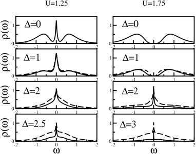
Figure 4: LDOS for $U=1.25$ (left column) and $U=1.75$ (right column) for different disorder strengths $\Delta$. Solid (dashed) curves correspond to the geometrically (arithmetically) averaged LDOS.

The main result of this Letter is the ground state phase diagram of the Anderson–Hubbard model at half-filling shown in Fig. 1. Two different phase transitions are found to take place: a Mott-Hubbard MIT for weak disorder $\Delta$, and an Anderson MIT for weak interaction $U$. The two insulating phases surround the correlated, disordered metallic phase. The properties of these phases, and the transitions between them, will now be discussed.

(i) Metallic phase: The correlated disordered metallic phase is characterized by a non–zero value of $\rho_{\rm{geom}}(0)$, the spectral density at the Fermi level ($\omega=0$). Without disorder DMFT predicts this quantity is to be given by the bare DOS $N_{0}(0)$, as expressed by the Luttinger theorem muller89 . This means that Landau quasiparticles are well–defined at the Fermi level. The situation changes dramatically when randomness is introduced, since a subtle competition between disorder and electron interaction arises. Increasing disorder at fixed $U$ reduces $\rho_{\rm{geom}}(0)$ and thereby decreases the metallicity as shown in the upper panel of Fig. 2. The opposite behavior is found when the interaction is increased at fixed $\Delta$ (see Fig. 3 for $\Delta=1$), i.e., the metallicity improves in this case. In the strongly interacting metallic regime the value of $\rho_{\rm{geom}}(0)$ is restored, reaching again its maximal value $N_{0}(0)$. Physically this means that in the metallic phase sufficiently strong interactions protect the quasiparticles from their decay due to impurity scattering. For weak disorder this effect of the interaction is essentially independent of the choice of the LDOS.

(ii) Mott-Hubbard MIT: For weak to intermediate disorder there is a sharp transition at a critical value of $U$ between a correlated metal and a gapped Mott insulator. We find two transition lines depending on whether the MIT is approached from the metallic side [$\Delta^{MH}_{c2}(U)$, full dots in Fig. 1] or from the insulating side [$\Delta^{MH}_{c1}(U)$, open dots in Fig. 1]. This is very similar to the case without disorder rozenberg94 ; georges96 ; bulla99 ; the hysteresis is clearly seen in Fig. 3 for $\Delta=1$. The $\Delta^{MH}_{c1}(U)$ and $\Delta^{MH}_{c2}(U)$ curves in Fig. 1 have positive slope. This is a consequence of the disorder–induced increase of spectral weight at the Fermi level (see Fig. 4) which in turn requires a stronger interaction to open the correlation gap. In the Mott insulating phase close to the hysteretic region an increase of disorder will therefore drive the system back into the metallic phase. The corresponding abrupt rise of $\rho_{\rm{geom}}(0)$ is seen in the lower panel of Fig. 2 and the right column of Fig. 4. In this case the disorder protects the metal from becoming a Mott insulator.

Around $\Delta\approx 1.8$ the $\Delta^{MH}_{c1}(U)$ and $\Delta^{MH}_{c2}(U)$ curves terminate at a single critical point, cf. Fig. 1. At stronger disorder ($\Delta\gtrsim 1.8$) only a smooth crossover from a metal to an insulator takes place. This is clearly illustrated by the $U$ dependence of $\rho_{\rm{geom}}(0)$ shown in Fig. 3 for $\Delta=2.5$. In this parameter regime the Luttinger theorem is not obeyed for any $U$. In the crossover regime, marked by the hatched area in Fig. 1, $\rho_{\rm{geom}}(0)$ vanishes gradually, so that the metallic and insulating phases can no longer be distinguished rigorously bulla01 .

Qualitatively, we find again that the Mott-Hubbard MIT and the crossover region do not depend much on the choice of the average of the LDOS. We also note the similarity between the Mott-Hubbard MIT scenario discussed here and the one for the system without disorder at finite temperatures georges93 ; rozenberg94 ; bulla01 , especially the presence of a coexistence region with hysteresis. However, while in the non–disordered case the interaction needed to trigger the Mott-Hubbard MIT decreases with increasing temperature, the opposite holds in the disordered case.

(iii) Anderson MIT: In Fig. 1 the metallic phase and the crossover regime are seen to lie next to an Anderson insulator phase where the LDOS of the extended states vanishes completely. The critical disorder $\Delta^{A}_{c}(U)$ corresponding to the Anderson MIT is a non–monotonous function of the interaction: it increases in the metallic regime and decreases in the crossover regime. Where $\Delta^{A}_{c}(U)$ has a positive slope an increase of the interaction turns the Anderson insulator into a correlated metal. This is illustrated in Fig. 3 for $\Delta=2.5$: at $U/W\approx 0.7$ a transition from a localized to a metallic phase occurs, i.e., the spectral weight at the Fermi level becomes finite. In this case the electronic correlations impede the localization of quasiparticles due to impurity scattering.

Fig. 2 shows that the Anderson MIT is continuous. In the critical regime $\rho_{\rm{geom}}(0)\sim[\Delta^{A}_{c}(U)-\Delta]^{\beta}$ for $U=\rm{const}$. In the crossover regime we find a critical exponent $\beta=1$ (see the case $U=1.75$ in lower panel of Fig. 2); elsewhere $\beta\neq 1$. However, since it is difficult to determine $\beta$ with high accuracy we cannot rule out a very narrow critical regime with $\beta=1.$ It should be stressed that an Anderson transition with vanishing $\rho_{\rm{geom}}(0)$ at finite $\Delta=\Delta^{A}_{c}(U)$ can only be detected in DMFT when the geometrically averaged LDOS is used (solid lines in Fig. 2). With arithmetic averaging one finds a nonvanishing LDOS at any finite $\Delta$ (dashed lines in Fig. 2).

(iv) Mott and Anderson insulators: The Mott insulator with a correlation gap is rigorously defined only for $\Delta=0$, and the gapless Anderson insulator only for $U=0$ and $\Delta>\Delta^{A}_{c}(0)$. In the presence of interaction and disorder this distinction can no longer be made. However, as long as the LDOS shows the characteristic Hubbard subbands (see left inset in Fig. 3) one may refer to a disordered Mott insulator. With increasing $\Delta$ the spectral weight of the Hubbard subbands vanishes (see right inset in Fig. 3) and the system becomes a correlated Anderson insulator. The border between these two types of insulators is marked by a dashed line in Fig. 1. The results obtained here within DMFT prove that the paramagnetic Mott and Anderson insulators are continuously connected. Hence, by changing $U$ and $\Delta$ it is possible to move from one type of insulator to the other without crossing the metallic phase.

In conclusion, using DMFT with the geometrically averaged (typical) LDOS we computed the non–magnetic ground state phase diagram of the Anderson–Hubbard model at half–filling for arbitrary interaction and disorder strengths. In particular, we determined the position of the Mott–Hubbard metal-insulator and Anderson localization transitions. The presence of disorder increases the critical interaction for the Mott-Hubbard MIT, and turns the sharp transition (with hysteresis) into a smooth but rapid crossover. On the other hand, the critical disorder strength for Anderson localization increases for weak interaction and is suppressed by strong interactions. The paramagnetic Mott and Anderson insulators are continuously connected. The specific predictions of our theory not only apply to disordered solids but also to cold fermionic atoms in optical lattices optical . In the latter case a precise control of system parameters appears to be possible which, in principle, allows one to explore all parts of the phase diagram.

We thank R. Bulla, S. Kehrein, R. Kutner, D. Lobaskin, and J. Tworzydło for useful discussions. This work was supported in part by the Sonderforschungsbereich 484 of the Deutsche Forschungsgemeinschaft (DFG). Financial support of KB through KBN-2 P03B 08 224, and of WH through the DFG and a Pappalardo Fellowship is gratefully acknowledged.

References

- (1) P. A. Lee and T. V. Ramakrishnan, Rev. Mod. Phys. 57, 287 (1985); D. Belitz and T. R. Kirkpatrick, Rev. Mod. Phys. 66, 261 (1994).
- (2) N. F. Mott, Proc. Phys. Soc. A 62, 416 (1949); Metal–Insulator Transitions, 2nd edn. (Taylor and Francis, London 1990).
- (3) P. W. Anderson, Phys. Rev. 109, 1492 (1958).
- (4) S. V. Kravchenko et al., Phys. Rev. B 50, 8039 (1994); D. Popović, A. B. Fowler, and S. Washburn, Phys. Rev. Lett. 79, 1543 (1997); S. V. Kravchenko and M. P. Sarachik, cond-mat/0309140; H. von Löhneysen, Adv. in Solid State Phys. 40, 143 (2000).
- (5) A. M. Finkelshtein, Sov. Phys. JEPT 75, 97 (1983); C. Castellani et al., Phys. Rev. B 30, 527 (1984); M. A. Tusch and D. E. Logan, Phys. Rev. B 48, 14843 (1993); ibid. 51, 11940 (1995); D. L. Shepelyansky, Phys. Rev. Lett. 73, 2607 (1994); P. J. H. Denteneer, R. T. Scalettar, and N. Trivedi, Phys. Rev. Lett. 87, 146401 (2001).
- (6) The most probable value of a random quantity is defined as that value for which its PDF becomes maximal.
- (7) A. D. Mirlin and Y. V. Fyodorov, Phys. Rev. Lett. 72, 526 (1994); J. Phys. I France 4, 655 (1994); M. Janssen, Phys. Rep. 295, 1 (1998) and references therein.
- (8) D. Lloyd, J. Phys. C2, 1717 (1969); D. Thouless, Phys. Reports 13, 93 (1974); F. Wegner, Z. Phys. B 44, 9 (1981).
- (9) Log-normal distribution–theory and applications, ed. E. L. Crow and K. Shimizu (Marcel Dekker, inc. 1988).
- (10) E. W. Montroll and M. F. Schlesinger, J. Stat. Phys. 32, 209 (1983); M. Romeo, V. Da Costa, and F. Bardou, Eur. Phys. J. B 32, 513 (2003).
- (11) V. Dobrosavljević and G. Kotliar, Phys. Rev. Lett. 78, 3943 (1997).
- (12) V. Dobrosavljević, A. A. Pastor, and B. K. Nikolić, Europhys. Lett. 62, 76 (2003).
- (13) G. Schubert, A. Weiße, and H. Fehske, cond-mat/0309015.
- (14) W. Metzner and D. Vollhardt, Phys. Rev. Lett. 62, 324 (1989).
- (15) A. Georges et al., Rev. Mod. Phys. 68, 13 (1996).
- (16) M. Ulmke, V. Janiš, and D. Vollhardt, Phys. Rev. B 51, 10411 (1995).
- (17) R. Vlaming and D. Vollhardt, Phys. Rev. B 45, 4637 (1992).
- (18) F. X. Bronold, A. Alvermann, and H. Fehske, Phil. Mag. 84, 637 (2004).
- (19) For a uniform PDF and discrete values of one finds . Hence vanishes if any of the is zero. The arithmetic average does not have such a property.
- (20) For numerical integrations we use discrete values of selected according to the Gauss-Legendre algorithm ulmke95 .
- (21) K. G. Wilson, Rev. Mod. Phys. 47, 773 (1975); T. A. Costi, A. C. Hewson, and V. Zlatić, J. Phys.: Cond. Mat. 6, 2519 (1994); R. Bulla, A. C. Hewson, and Th. Pruschke, J. Phys.: Condens. Matter 10, 8365 (1998); W. Hofstetter, Phys. Rev. Lett. 85, 1508 (2000).
- (22) R. Bulla, Phys. Rev. Lett. 83, 136 (1999).
- (23) E. Müller-Hartmann, Z. Phys. B 76, 211 (1989).
- (24) M. J. Rozenberg, G. Kotliar, and X. Y. Zhang, Phys. Rev. B 49, 10181 (1994).
- (25) R. Bulla, T. A. Costi, and D. Vollhardt, Phys. Rev. B 64, 045103 (2001)
- (26) A. Georges and W. Krauth, Phys. Rev. B 48, 7167 (1993).
- (27) W. Hofstetter et al., Phys. Rev. Lett. 89, 220407 (2002); P. Horak, J. Y. Courtois, and G. Grynberg, Phys. Rev. A 58, 3953 (1998); R. Roth and K. Burnett, J. Opt. B: Quantum Semiclassical Opt. 5, S50 (2003).