The aim of this paper is to present a stochastic model that accounts for the effects of a long-memory in volatility on option pricing. The starting point is the stochastic Black-Scholes equation involving volatility with long-range dependence. We define the stochastic option price as a sum of classical Black-Scholes price and random deviation describing the risk from the random volatility. By using the fact that the option price and random volatility change on different time scales, we derive the asymptotic equation for this deviation involving fractional Brownian motion. The solution to this equation allows us to find the pricing bands for options.

Keywords: Long memory, stochastic volatility, option pricing

1 Introduction

Over the last few years, self-similarity and long-range dependence have become important concepts in analyzing the financial time series [1, 2]. There is strong evidence that the return, $r_{t},$ has little or no autocorrelation, whereas its square, $r_{t}^{2},$ or absolute return, $|r_{t}|,$ exhibit noticeable autocorrelation [3]. This phenomenon can be described by the ARCH(p) model [4] or its GARCH(p,q) extension [5]. However, the exponential decay for $\lambda_{s}=cov(r_{t}^{2},r_{t+s}^{2})$ is believed to be too fast to describe correctly the persistent dependence between the series observations as the time lag increases. It turns out [6, 7] that the models with hyperbolic decay which have slowly decaying covariances provide better fitting to financial time series. The characteristic feature of these models is that their covariance $\lambda_{s}$ has the power law decay $s^{2d-1}$ ($0<d<1/2)$ for the large lag $s$ such that

$$\sum\limits_{s=0}^{\infty}\lambda_{s}=\infty\text{ }.$$ (1)

The financial series is said to have long memory if it displays this property [7]. This means that the square of returns that are far apart are strongly correlated, since the correlations decay very slowly to zero. Let us note that the series is said to have short memory if the autocovarience is summable. Evidences for long memory in daily absolute or squared returns have been well documented (see, for example, [8, 9, 10]). The review of long memory models leading to (1) can be found in [7].

The natural question arises: what is the implication of this long-range dependence in volatility on the option pricing. It is well known that the existence of ‘smile’ and ‘frown’ in the implied volatility graph contradicts the Black-Scholes assumption of constant volatility. To remedy this shortcoming, many stochastic volatility models have been proposed (see, for example, [11, 12, 13]). Despite the large volume of literature discussing stochastic volatility, the effects of long-memory on option pricing are relatively unexplored. Several attempts have been made to understand the role of long-range dependence in volatility on derivative pricing. Comte and his colleagues generalized the classical Heston model to account for long memory features of stochastic volatility [14, 15]. The main idea was to define the volatility process as the fractional integration of the short memory process. The main difficulty with this approach is that the volatility is not a directly tradeable asset, and therefore the classical Black-Scholes hedging can not be applied. It leads to the appearance of an unknown parameter, namely, the market price of volatility risk [11, 12]. The problem is that this parameter is not directly observable and one has to make additional assumptions regarding the pricing of volatility risk. An extension of the Stein and Stein model for a long memory volatility case was given in [16], where the option price was obtained through a risk-minimization procedure (see also other works [17, 18]). A different approach to option pricing with stochastic volatility has been suggested in [19]. Instead of finding the exact option price the authors focused on the pricing bands for options that account for the random volatility risk. However, they considered only weakly correlated random volatility and did not discuss the long memory effects. Stochastic volatility can be also treated by a stochastic optimization approach based on a risk minimization procedure [20].

It is the purpose of this paper to present a simple stochastic volatility model that accounts for the long memory effects of stochastic volatility on option pricing. We start with the classical Black-Scholes equation with random volatility which has long-range dependence. The aim is to find the option price as a sum of Black-Scholes price with average volatility and random deviation describing the risk from random volatility. A main feature of this approach is that it does not need an estimation of the market price volatility risk [19].

It should be noted that there exists a family of continuous random processes which capture the long memory property including the well-known fractional Brownian motion (fBm) [21]. A substantial amount of research has been done in an attempt to model the stock return (see, for example, [22] and the references therein). In particular, it has been shown that the simple replacement of the Wiener process by fBm leads to arbitrage opportunities in the market [23]. Recall that the fractional Brownian motion with Hurst coefficient $H$ is the Gaussian process $B_{d}(t)$ with mean $E\left\{B_{d}(t)\right\}=0$ and covariance [21]

$$E\left\{B_{d}(t)B_{d}(s)\right\}=\frac{1}{2}(t^{2d+1}+s^{2d+1}-|t-s|^{2d+1}),$$ (2)

where $d$ is the difference parameter: $d=H-1/2,$ and $E$ denotes the expectation. In particular, it follows from (2) that $E\{B_{d}^{2}\}=t^{1+2d}$. If $H=1/2$ $(d=0)$, then $B_{d}(t)$ is identical to the standard Brownian motion $B(t).$ If $1/2<H<1$ $(0<d<1/2),$ then $B_{d}(t)$ has a long-range dependence in the sense that the sequence of increments $g_{d}(n)=B_{d}(n)-$ $B_{d}(n-1)$ is strongly correlated, namely, $E\{g_{d}(n)g_{d}(n+k)\}\sim k^{2d-1}$ as $k\rightarrow\infty.$ The stochastic calculus for fractional Brownian motion for the Hurst exponent in the interval $(1/2,1)$ is given in [24]

2 Incorporation of long memory volatility into the option pricing model

We start with the Black-Scholes equation with the random volatility $\sigma(t),$

$$\frac{\partial C}{\partial t}+\frac{1}{2}\sigma^{2}(t)S^{2}\frac{\partial^{2}C}{\partial S^{2}}+rS\frac{\partial C}{\partial S}-rC=0,$$ (3)

where $C$ is the call option price, $r$ is the interest rate, and $t$ is the time ($0\leq t\leq T$). We adopt the idea that the volatility’s time variations are small compared with time scale of the option [19]. We assume that $\sigma^{2}(t)$ is the stationary long memory process with the following statistical characteristics:

$$E\{\sigma^{2}(t)\}=\overline{\sigma^{2}},\;\;\;E\{(\sigma^{2}(t)-\overline{\sigma^{2}})(\sigma^{2}(t+s)-\overline{\sigma^{2}})\}=g(s)=\frac{c}{(s_{0}+s)^{\alpha}},$$ (4)

where $E\{\cdot\}$ is the expectation, $g(s)$ is the covariance, and the parameter $\alpha$ obeys

$$0<\alpha<1.$$ (5)

It follows from (4) that for large lag $s,$ the covariance $g(s)$ decreases to zero like a power law $s^{-\alpha},$ while the spectrum $\rho\left(\lambda\right)$ goes to infinity at the origin [7]

$$\rho(\lambda)\sim\frac{c_{\rho}}{\lambda^{1-\alpha}}\;\;\;\text{as}\;\;\;\lambda\rightarrow 0.$$ (6)

The parameter $\alpha$ can be regarded as a measure of the intensity of the long-range dependence of the volatility. A variety of techniques are available to estimate the parameter $\alpha$ from financial time series (see [7]). The characteristic feature of (4) is that the integral $\int_{0}^{t}g(s)ds$ diverges as $t\rightarrow\infty.$

We should remark that our assumption that the typical time scales of volatility variations are small compared with the time scale of the derivative contract is not inconsistent with the long memory properties of the volatility (4). A similar situation occurs in the renormalization theory of turbulent diffusivity in which the random velocity field with a power law spectrum involves a continuous range of time/space scales and all of them are less than the integral scales (see [28]). If we assume that the time variable $t$ is measured in $t_{d}$ units (several days), then the spectrum $\rho_{\varepsilon}(\lambda)$ can be written as follows

$$\rho_{\varepsilon}(\lambda)\sim\frac{c_{\rho}}{\lambda^{1-\alpha}}\;\;\;\text{for}\;\;\;\varepsilon<\lambda<<1,\;\;\;\rho_{\varepsilon}(\lambda)=0\;\;\;\text{for}\;\;\;0\leq\lambda\leq\varepsilon,$$ (7)

where $\varepsilon$ is the small parameter

$$\varepsilon=\frac{t_{d}}{T}.$$ (8)

The spectrum (7) describes the situation when there are no time-scales in $\sigma^{2}(t)$ greater than the expiry date $T.$ One can also write this using the infrared cut-off function $\psi_{0}:$ the spectrum $\rho_{\varepsilon}(\lambda)$ can be represented as $\rho_{\varepsilon}(\lambda)\sim\frac{c_{\rho}}{\lambda^{1-\alpha}}\psi_{0}\left(\frac{\lambda}{\varepsilon}\right)$, where $\psi_{0}=1$ for $\lambda>\varepsilon$ and $\psi_{0}=0$ for $\lambda\leq\varepsilon.$ This idea was introduced by Avellaneda and Majda in [28], where they analyzed turbulent transport for a random velocity with a power law spectrum. Of course, in the limit $\varepsilon\rightarrow 0$ the spectrum, $\rho_{\varepsilon}(\lambda)$ tends to $\rho(\lambda)$ which leads to the infrared divergence of corresponding integrals. In what follows we consider only the asymptotic regime $\varepsilon\rightarrow 0,$ therefore one can use the idealized spectrum function $\rho(\lambda)$ instead of $\rho_{\varepsilon}(\lambda)$ with the infrared cut-off. The details concerning the renormalization procedure, non-trivial scaling and infrared divergent integrals can be found in [28].

To deal with the forward problem we introduce the time-to-maturity

$$\tau=T-t$$ (9)

and measure it in terms of one-year units. The stochastic volatility $\sigma(\tau)$ becomes a rapidly fluctuating function. It is convenient to split $\sigma^{2}(\tau)$ into the mean value, $\overline{\sigma^{2}},$ and a rapidly varying component, $v,$ as follows

$$\sigma^{2}(\tau)=\overline{\sigma^{2}}+v\left(\frac{\tau}{\varepsilon}\right).$$ (10)

It is evident that the autocorrelation function for $v$ is given by $g(s)$ (see (4)). Using (9) and (10), we find that the corresponding stochastic option price $C^{\varepsilon}(\tau,S)$ satisfies the following stochastic PDE:

$$\frac{\partial C^{\varepsilon}}{\partial\tau}=\frac{1}{2}\overline{\sigma^{2}}S^{2}\frac{\partial^{2}C^{\varepsilon}}{\partial S^{2}}+\frac{1}{2}v\left(\frac{\tau}{\varepsilon}\right)S^{2}\frac{\partial^{2}C^{\varepsilon}}{\partial S^{2}}+rS\frac{\partial C^{\varepsilon}}{\partial S}-rC^{\varepsilon}$$ (11)

subject to the initial condition

$$C^{\varepsilon}(0,S)=\max(S-K,0),$$ (12)

where $K$ is the strike price.

Our purpose now is to analyze the asymptotic behavior of $C^{\varepsilon}(\tau,S)$ as $\varepsilon\rightarrow 0.$ We split the option price $C^{\varepsilon}(\tau,S)$ into the sum of the deterministic price, $\overline{C}(\tau,S),$ and the random deviation, $Z^{\varepsilon}(\tau,S),$ with the anomalous scaling factor, $\varepsilon^{1/2-d},$ to get

$$C^{\varepsilon}(\tau,S)=\overline{C}(\tau,S)+\varepsilon^{1/2-d}Z^{\varepsilon}(\tau,S),$$ (13)

where $\overline{C}(\tau,S)$ is the classical Black-Scholes price, which satisfies [25, 26]

$$\frac{\partial\overline{C}}{\partial\tau}=\frac{1}{2}\overline{\sigma^{2}}S^{2}\frac{\partial^{2}\overline{C}}{\partial S^{2}}+rS\frac{\partial\overline{C}}{\partial S}-r\overline{C}.$$ (14)

Note that the case $d=0$ corresponds to the short memory volatility model considered in [19]. In this paper we assume that the parameter $d$ varies in the range:

$$0<d<\frac{1}{2}.$$ (15)

The expression for the parameter $d$ in terms of $\alpha$ is derived in Appendix A (see (A-4)):

$$d=\frac{1-\alpha}{2}.$$ (16)

Substituting (13) into (11) and using (14), we get the equation for $Z^{\varepsilon}(\tau,S)$

$$\frac{\partial Z^{\varepsilon}}{\partial\tau}=\frac{1}{2}\overline{\sigma^{2}}S^{2}\frac{\partial^{2}Z^{\varepsilon}}{\partial S^{2}}+\frac{1}{2}v\left(\frac{\tau}{\varepsilon}\right)S^{2}\frac{\partial^{2}Z^{\varepsilon}}{\partial S^{2}}+rS\frac{\partial Z^{\varepsilon}}{\partial S}-rZ^{\varepsilon}+\frac{1}{2}\varepsilon^{-1/2+d}v\left(\frac{\tau}{\varepsilon}\right)S^{2}\frac{\partial^{2}\overline{C}}{\partial S^{2}}.$$ (17)

Our objective now is to find the asymptotic limit of $Z^{\varepsilon}(\tau,S)$ as $\varepsilon\rightarrow 0.$ The equation (17) involves two stochastic terms:

$$\frac{1}{2}v\left(\frac{\tau}{\varepsilon}\right)S^{2}\frac{\partial^{2}Z^{\varepsilon}}{\partial S^{2}},\;\;\;\;\;\;\frac{1}{2}\varepsilon^{-1/2+d}v\left(\frac{\tau}{\varepsilon}\right)S^{2}\frac{\partial^{2}\overline{C}}{\partial S^{2}}.$$ (18)

Ergodic theory implies that the first term in its integral form converges to zero as $\varepsilon\rightarrow 0,$ while the second term converges weakly to

$$\frac{1}{2}D_{d}^{1/2}\xi_{d}(\tau)S^{2}\frac{\partial^{2}\overline{C}}{\partial S^{2}}\;\;as\text{ }\;\;\varepsilon\rightarrow 0,$$ (19)

where $\xi_{d}(\tau)$ is the fractional Gaussian white noise

$$\xi_{d}(\tau)=\frac{dB_{d}}{d\tau}$$ (20)

with the covariance [22, 24]

$$E\{\xi_{d}(\tau)\xi_{d}(s)\}=d(2d+1)|\tau-s|^{2d-1}.$$ (21)

Here, $B_{d}$ is the fractional Brownian motion (2) and $D_{d}$ is given by

$$D_{d}=\frac{2c}{(1-\alpha)(2-\alpha)},\;\;0<\alpha<1$$ (22)

(derivation of $D_{d}$ can be found in the Appendix A). The limit (19) follows from [27]

$$\varepsilon^{-1/2+d}\int_{0}^{\tau}v\left(\frac{s}{\varepsilon}\right)ds\rightarrow D_{d}^{1/2}B_{d}(\tau)\;\;as\text{ }\;\;\varepsilon\rightarrow 0.$$ (23)

Thus the random field $Z^{\varepsilon}(\tau,S)$ converges weakly to $Z(\tau,S)$ which obeys the asymptotic equation

$$\frac{\partial Z}{\partial\tau}=\frac{1}{2}\overline{\sigma^{2}}S^{2}\frac{\partial^{2}Z}{\partial S^{2}}+rS\frac{\partial Z}{\partial S}-rZ+\frac{1}{2}D_{d}^{1/2}S^{2}\frac{\partial^{2}\overline{C}}{\partial S^{2}}\xi_{d}(\tau).$$ (24)

with the initial condition $Z(0,S)=0$.

In this paper we present only a heuristic derivation of the limiting equation (24). The rigorous derivation should involve the exact renormalization technique together with stochastic averaging and the central limit theorem for stochastic processes [28, 29]. It should be noted that Eq. (24) can be also rewritten in terms of the Black-Scholes operator

$$L_{BS}\left[Z\right]=\frac{1}{2}\overline{\sigma^{2}}S^{2}\frac{\partial^{2}Z}{\partial S^{2}}+rS\frac{\partial Z}{\partial S}-rZ$$ (25)

and the fractional Brownian motion $B_{d},$ as follows:

$$dZ=L_{BS}\left[Z\right]dt+\frac{1}{2}D_{d}^{1/2}S^{2}\frac{\partial^{2}\overline{C}}{\partial S^{2}}dB_{d}.$$ (26)

The advantage of the asymptotic equation (24) is that it can be solved in terms of the classical Green’s function, $G(S,S_{1},\tau,\tau_{1}),$ for the Black-Scholes equation [26]. It follow from (24) that [30]

$$Z(\tau,S)=\frac{1}{2}D_{d}^{1/2}\int_{0}^{\tau}\int_{0}^{\infty}G(S,S_{1},\tau,\tau_{1})S_{1}^{2}\frac{\partial^{2}\overline{C}}{\partial S^{2}}(\tau_{1},S_{1})\xi_{d}(\tau_{1})dS_{1}d\tau_{1},$$ (27)

where $G(S,S_{1},\tau,\tau_{1})$ is

$$G(S,S_{1},\tau,\tau_{1})=\frac{e^{-r(\tau-\tau_{1})}}{S_{1}\sqrt{2\pi\overline{\sigma^{2}}(\tau-\tau_{1})}}\exp\left(-\frac{[\ln(S/S_{1})+(r-\frac{\overline{\sigma^{2}}}{2})(\tau-\tau_{1})]^{2}}{2\overline{\sigma^{2}}(\tau-\tau_{1})}\right).$$ (28)

The variance

$$V(\tau,S)=E\{Z^{2}(\tau,S)\}$$ (29)

can be regarded as a measure of volatility risk. It can be easily found from (27) that

$$V(\tau,S)=\frac{1}{4}D_{d}\int_{0}^{\tau}\int_{0}^{\tau}\int_{0}^{\infty}\int_{0}^{\infty}G(S,S_{1},\tau,\tau_{1})G(S,S_{2},\tau,\tau_{2})$$ (30)

$$\times S_{1}{}^{2}S_{2}{}^{2}\frac{\partial^{2}\overline{C}}{\partial S^{2}}\left(\tau_{1},S_{1}\right)\frac{\partial^{2}\overline{C}}{\partial S^{2}}(\tau_{2},S_{2})E\{\xi_{d}(\tau_{1})\xi_{d}(\tau_{2})\}dS_{1}dS_{2}d\tau_{1}d\tau_{2},$$

where

$$E\{\xi_{d}(\tau_{1})\xi_{d}(\tau_{2})\}=d(2d+1)|\tau_{1}-\tau_{2}|^{2d-1}.$$ (31)

It should be noted that despite the fact that $\xi_{d}(\tau)$ converges to the Gaussian white noise as $d\rightarrow 0$ and

$$\lim_{d\rightarrow 0}E\{\xi_{d}(\tau_{1})\xi_{d}(\tau_{2})\}=\delta(\tau_{1}-\tau_{2}),$$ (32)

we cannot consider the short memory case ($d=0)$ for (30). The problem is that in the limit $d\rightarrow 0$ ($D_{d}\rightarrow\infty)$ we have logarithmic divergence of time integrals (see Appendix A) . Recall that in the Gaussian white noise case the variance $V(\tau,S)=$ $E\{Z^{2}(\tau,S)\}$ has the following expression [19]

$$V(\tau,S)=\frac{D}{4}\int_{0}^{\tau}\left(\int_{0}^{\infty}G(S,S_{1},\tau,\tau_{1})S_{1}^{2}\frac{\partial^{2}\overline{C}}{\partial S_{1}^{2}}dS_{1}\right)^{2}d\tau_{1}.$$ (33)

It should be noted that the main result concerning the measure of volatility risk (30) is very robust. The main reason for this is that for the random volatility $\sigma^{2}(t)$ we use a quite general stationary random process (4) without assuming the exact distributions for it, like Gaussian, Poisson, etc. It is very important because there is empirical evidence that the volatility is not Gaussian and its probability density function can have power-law tails [31]. Of course after rescaling the central limit theorem insures in the asymptotic limit $\varepsilon\rightarrow 0$ effective volatility becomes Gaussian. It follows from (4) that the value of the covariance $g(s)$ at $s=0$ is finite. One can consider the situation when this is not the case. Then we should apply a different scaling procedure which will lead to a stable distribution with the power-law tails in the asymptotic limit [32].

3 Numerical Results

In this section we present numerical results for the variance of $C^{\varepsilon}(\tau,S)$

$$E\left\{\left(C^{\varepsilon}(\tau,S)-\overline{C}(\tau,S)\right)^{2}\right\}=\varepsilon^{1-2d}V(\tau,S)$$ (34)

for the different values of $d$. Assume that the exercise price of the call option is $\$50$, the risk-free interest rate is $5\%$ p.a., and the average volatility is $20\%$ p.a., that is, $K=50,$ $r=0.05,$ $\overline{\sigma^{2}}=0.04.$ Figure 1 shows the graph of the variance $E\left\{\left(C^{\varepsilon}(\tau,S)-\overline{C}(\tau,S)\right)^{2}\right\}$plotted against the stock price $S$ for $\tau=0.5$ , $\varepsilon=0.1$ and $d=0.01$, $0.1$, $0.3$, and $0.45$ respectively ($c=1$).

From Figure 1 we can see that for at-the-money call option there is maximum uncertainty since all graphs have a maximum near $S=K,$ where $K$ is the strike price. As for deep in- and out-the-money option there is almost zero uncertainty. It should be noted that the strength of the memory effect is determined by the value of the parameter $d.$ One can see from Figure 1 that the increase in $d$ leads to an increase in the variance and therefore in the risk value. If we assume as in, [19], that the writer sells the option for

$$\overline{C}(\tau,S)+2\varepsilon^{1/2-d}V^{1/2}(\tau,S)$$ (35)

then the increase in parameter the $d$ leads to the increase in option price. In Figure 2, we plot 3-dimensional graphs of the variance $E\left\{\left(C^{\varepsilon}(\tau,S)-\overline{C}(\tau,S)\right)^{2}\right\}$against the stock price $S$ and time to maturity $\tau$ for $d=0.3$ and $d=0.1.$ Note that the variance increases with the time to maturity. It should be noted that these results are similar to those obtained in [33]. It was found that the residual risk vanishes for both deep in-the-money options and deep out-of-the money options, but increases sharply for at-the-money option.

4 Conclusion

In this paper we presented a stochastic model that accounts for the effects of a long-memory in volatility on option pricing. We started with the random Black-Scholes equation with the volatility parameter being the stationary random process with long-range dependence. We represented the option price as a sum of classical Black-Scholes price and random deviation describing the risk from the random volatility. By using the renormalization procedure we derived the asymptotic equation for this deviation. By using Green’s function methods we solved this equation and found the asymptotic pricing bands for options.

From numerical calculations of the variance of the random option price we found that the maximum deviation from the classical Black-Scholes price takes place for at-the-money option, while the risk due to random volatility vanishes both for deep-in and out-of-the-money options. We also found that the increase in the strength of the memory effect leads to an increase in the variance and therefore in the effective option price.

Appendix A

Weak convergence to fractional Brownian motion

The purpose of this Appendix is to derive the expressions for the parameters $D_{d}$ and $d$ by using the autocorrelation function

$$g(s)=\;E\{v(\tau)v(\tau+s)\}=\frac{c}{(s_{0}+s)^{\alpha}},\;\;\;0<\alpha<1.$$ (A-1)

Let us define the process $x^{\varepsilon}(\tau)$ as follows:

$$x^{\varepsilon}(\tau)=\varepsilon^{-\frac{1}{2}+d}\int_{0}^{\tau}v\left(\frac{s}{\varepsilon}\right)ds=\varepsilon^{\frac{1}{2}+d}\int_{0}^{\frac{\tau}{\varepsilon}}v(s)ds.$$ (A-2)

It converges weakly to the scaled fractional Brownian motion $D_{d}^{1/2}B_{d}$ as $\varepsilon\rightarrow 0.$ To derive expressions for $D_{d}$ and $d$, we show that

$$\lim_{\varepsilon\rightarrow 0}E\{[x^{\varepsilon}(\tau)]^{2}\}=D_{d}\tau^{2d+1},$$ (A-3)

where

$$D_{d}=\frac{2c}{(1-\alpha)(2-\alpha)},\;\;d=\frac{1-\alpha}{2}.$$ (A-4)

It follows from (A-1) and (A-2) that

$$E\{[x^{\varepsilon}(\tau)]^{2}\}=\varepsilon^{1+2d}\int_{0}^{\frac{\tau}{\varepsilon}}\int_{0}^{\frac{\tau}{\varepsilon}}g(s_{1}-s_{2})ds_{1}ds_{2}.$$ (A-5)

By using the well-known formula for stationary process $v(s)$ with zero mean and the covariance function $g(s)$

$$\int_{0}^{\tau}\int_{0}^{\tau}E\{v(s_{1})v(s_{2})\}ds_{1}ds_{2}=\int_{0}^{\tau}\int_{0}^{\tau}g(s_{1}-s_{2})ds_{1}ds_{2}=2\tau\int_{0}^{\tau}g(s)ds-2\int_{0}^{\tau}sg(s)ds,$$ (A-6)

one finds that

$$E\{[x^{\varepsilon}(\tau)]^{2}\}=2\varepsilon^{1+2d}\left(\frac{\tau}{\varepsilon}\int_{0}^{\frac{\tau}{\varepsilon}}g(s)ds-\int_{0}^{\frac{\tau}{\varepsilon}}sg(s)ds\right).$$ (A-7)

In the long memory case ( $0<\alpha<1)$ both integrals

$$\int_{0}^{\frac{\tau}{\varepsilon}}g(s)ds,\;\;\;\int_{0}^{\frac{\tau}{\varepsilon}}sg(s)ds$$ (A-8)

diverge as $\varepsilon\rightarrow 0.$ That is why we need here the appropriate scaling factor $\varepsilon^{1+2d}$ to ensure that $E\{x^{\varepsilon}(\tau)\}^{2}$ is finite for the fixed value of $\tau.$ By using (A-1) we find

$$\int_{0}^{\frac{\tau}{\varepsilon}}g(s)ds=\frac{c}{\left(1-\alpha\right)}\allowbreak\left[\left(\frac{s_{0}\varepsilon+\tau}{\varepsilon}\right)^{-\alpha}s_{0}+\left(\frac{s_{0}\varepsilon+\tau}{\varepsilon}\right)^{-\alpha}\tau\varepsilon^{-1}-s_{0}^{1-\alpha}\right]$$ (A-9)

and

$$\int_{0}^{\frac{\tau}{\varepsilon}}sg(s)ds = -\frac{c}{(1-\alpha)(2-\alpha)}\left(\frac{s_{0}\varepsilon+\tau}{\varepsilon}\right)^{-\alpha}$$ (A-11)

$$\left[\tau^{2}\varepsilon^{-2}\alpha+s_{0}\alpha\tau\varepsilon^{-1}-\tau^{2}\varepsilon^{-2}+s_{0}^{2}-\left(\frac{s_{0}\varepsilon+\tau}{\varepsilon}\right)^{\alpha}s_{0}^{2-\alpha}\right].$$

If we set

$$d=\frac{1-\alpha}{2},$$ (A-12)

we find from (A-7) that

$$\lim_{\varepsilon\rightarrow 0}E\{x^{\varepsilon}(\tau)\}^{2}=\frac{2c\tau^{2-\alpha}}{(1-\alpha)(2-\alpha)}$$ (A-13)

and therefore

$$D_{d}=\frac{2c}{(1-\alpha)(2-\alpha)}.$$ (A-14)

Figure 1: Plot of variance, $E{\left\{\left(C^{\varepsilon}(\tau,S)-\overline{C}(\tau,S)\right)^{2}\right\}}$ against stock price, $S$ for $d=0.01$, $d=0.1$, $d=0.3$ and $d=0.45$ with $K=50$ and $\tau=0.5.$

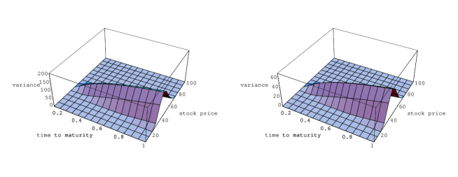
Figure 2: 3D-plot of variance, $E{\left\{\left(C^{\varepsilon}(\tau,S)-\overline{C}(\tau,S)\right)^{2}\right\}}$ against stock price, $S$ and time to maturity, $\tau$ for $d=0.3$ (left) and $d=0.1$ (right) with $K=50$ and $\tau=0.5.$

References

- [1] E. E. Peters, Fractal Market Analysis, John Willey & Sons (1994).
- [2] R. Mantegna and E. Stanley, Introduction to Econophysics, Cambridge University Press (1999)
- [3] J. Y. Campbell, A. W. Lo and A. Craig MacKinlay, The Econometrics of Financial Markets, Princeton Univ Press (1996).
- [4] R. F. Engle, Autoregressive Conditional Heteroskedasticity with Estimates of the Variance of the United Kingdom Inflation, Econometrica 50 (1982) 987 - 1007.
- [5] T. Bollerslev, Generalized autoregressive conditional heteroscedasticity, Journal of Econometrics 31 (1986) 307-327.
- [6] S. Poon and C. W. J. Granger, Forecasting volatility in financial markets, A Review, Journal of Economic Literature 41(2) (2003).
- [7] J. Beran, Statistics for long-memory processes, Chapman and Hall, New York, (1994).
- [8] Z. Ding, C. W. J. Granger and R. F. Engle, A Long Memory Properties of Stock Returns and a New Model, Journal of Empirical Finance 1 (1993) 83-106.
- [9] C. W. J. Granger and F. Marmol, The Correlogram of a Long Memory Process Plus a Simple Noise, UCSD Working Paper (1997).
- [10] F. Jay Breidt, N. Crato and P. D Lima, On the detection and estimation of long memory in stochastic volatility, Journal of Econonmetrics 83, (1998) 325-348.
- [11] J. P. Fouque, G. Papanicolaou, and K. R. Sircar, Derivatives in Financial Markets with Stochastic Volatility, Cambridge University Press (2000).
- [12] A. Lewis, Option Valuation under Stochastic Volatility, Finance Press, Newport Beach, CA (2000).
- [13] S. J. Taylor, Modelling stochastic volatility: A review and comparative study, Mathematical Finance 4 (1994) 183–204.
- [14] F. Comte and E. Renault, Long memory in continuous time stochastic volatility models, Mathematical Finance 8, (1998) 291-323.
- [15] F. Comte, L. Coutin and E. Renault, Affine fractional stochastic volatility models, Preliminary version (2001).
- [16] Y. Hu, Option pricing in a market where the volatility is driven by fractional Brownian motions, Recent Development on Mathematical Finance, World Scientific (2002), 49-59.
- [17] S. J. Taylor, Consequences for option pricing of a long memory in volatility, Working paper (2000).
- [18] B. Djehiche and M. Eddahbi, Hedging options in market models modulated by fractional Brownian motion. Stochastic Analysis and Applications, 19(5) (2001) 753-770.
- [19] G. C. Papanicolaou and K. R. Sircar, Stochastic Volatility, Smiles and Asymptotics, Applied Mathematical Finance 6 (1999), pp107-145.
- [20] S. Fedotov and S. Mikhailov, Option pricing for incomplete markets via stochastic optimization: transaction costs, adaptive control and forecast, Int. J. Theoretical and Applied Finance 4(1) (2001).
- [21] F. Comte and E. Renault, Long memory continuous time models, Journal of Econometrics 73 (1996) 101-149.
- [22] Y. Hu and B. Oksendal, Fractional white noise calculus and applications to finance, Infinite Dimensional Analysis, Quantum Probability and Related Topics, 6(1) (2003) 1-32.
- [23] L. C. G. Rogers, Arbitrage with Fractional Brownian Motion. Math. Finance 7 (1997) 95-105.
- [24] T. E. Duncan, Y. Hu, and B. Pasik-Duncan, Stochastic Calculus for Fractional Brownian Motion. I. Theory, SIAM J. Control Optim. 38 (2000) 582-612.
- [25] J. C. Hull, Options, Futures And Other Derivatives, 5th Edition, Prentice-Hall (2002).
- [26] P. Wilmott, S. Howison and J. Dewynne, The Mathematics of Financial Derivatives, A Student Introduction, Cambridge University Press (1999).
- [27] L. Giraitis, P. Kokoszka, R. Leipus and G. Teyssiere, Rescaled variance and related tests for long memory in volatility and levels. Journal of Econometrics 112 (2003) 265-294.
- [28] M. Avellaneda, and A. Majda, Mathematical Models with Exact Renormalization for Turbulent Transport, Commun. Math. Phys. 131, (1990) 381-429.
- [29] H. Watanabe, Averaging and fluctuations for parabolic equations with rapidly oscillating random coefficients. Prob. Th. Rel. Fields, 77 (1988) 358-378.
- [30] R. Courant, and D. Hilbert, Methods of Mathematical Physics, Volume II, Partial Differential Equations, Wiley (1989).
- [31] Y. Liu, P. Gopikrishnan, P. Cizeau, M. Meyer, C.-K. Peng, H. E. Stanley, Statistical properties of the volatility of price fluctuations, Phys. Rev. E, 60 (1999) 1390-1400.
- [32] G. Samorodnitsky and M. S. Taqqu, Stable Non-Gaussian Random Processes, Chapman&Hall, New York, 1994.
- [33] E. Aurel, and S. Simdyankin, Pricing risky options simply, Intern. J. Theor. Appl. Finance, 1 (1998) 1-23.