Nonequilibrium electron transport using the density matrix renormalization group

Abstract

We extended the Density Matrix Renormalization Group method to study the real time dynamics of interacting one dimensional spinless Fermi systems by applying the full time evolution operator to an initial state. As an example we describe the propagation of a density excitation in an interacting clean system and the transport through an interacting nano structure.

I Introduction

The density matrix renormalization group method (DMRG) DMRG:Base ; DMRG:Book is a powerful technique to study the properties of one dimensional interacting quantum systems. The advantage of the DMRG is that it can treat quantum lattice systems in the presence of site-dependent interaction, hopping parameter, and on-site potentials DMRG:Disorder with high accuracy, including subtle lattice effects like multiple umklapp processes.DMRG:MUS

Originally the method was set up to describe the equilibrium properties of the ground state and a few excited states. It was then extended to calculate frequency dependent spectral functions by the use of the $[H-E_{0}-\omega+\imath\eta]^{-1}$ operator.DMRG:SpktrlFkt-Hallberg ; DMRG:SpktrlFkt-White ; DMRG:SpktrlFkt-Jeckelmann

A second approach to study transport properties within the framework of DMRG is to relate equilibrium properties of the ground state to transport properties. Molina et al. DMRG:PC-Molina and Meden and Schollwöck DMRG:PC-Meden calculated the conductance through an interacting nano structure attached to leads by relating the conductance of the system to the ground state curvature, based on an idea by Sushkov.Sushkov01

Cazalilla and Marston TdDMRG:Marston used the basis states of the last DMRG sweeps to integrate the Schrödinger equation in real time. However, as shown by Luo, Xiang, and Wang,TdDMRG:MarstonComment their approach was inconsistent with the DMRG scheme, since they used a basis to integrate the Schrödinger equation which was only adapted to the $t=0$ state, neglecting the relevant states for $t>0$ during the DMRG sweeps.

II Calculation of the time evolution

Instead of integrating the time dependent Schrödinger equation numerically, we make use of the formal solution and apply the full time evolution operator

$${\cal U}(t_{2},t_{1})=\text{e}^{-\imath{\cal H}(t_{2}-t_{1})}$$ (1)

to calculate the time dependence of an initial state $|{\xi(0)}\rangle$

$$|{\xi(t)}\rangle={\cal U}(t,0)|{\xi(0)}\rangle\,,$$ (2)

where $\cal H$ is the Hamiltonian of the system of interest.

While the calculation of $\text{e}^{-\imath{\cal H}t}$ is not feasible for large matrix dimensions, one can calculate the action of a matrix exponential on a vector similar to the diagonalization of sparse matrices, where one cannot diagonalize the full matrix, but one can search for selected eigenvalues and eigenvectors. We apply a Krylov subspace approximation Saad98 to calculate the action of the matrix exponential in equation (1) on a state $|{\xi}\rangle$. We would like to encourage the reader interested in implementing a matrix exponential to study the excellent review by Moler and Van Loan MolerLoan03 and discourage the use of a Taylor expansion. In our implementation we make use of a Padé approximation from Expokit Expokit to calculate the dense matrix exponential in the Krylov subspace. In order to calculate $|{\xi(t)}\rangle$ up to a final time $T$, we discretize the time interval into $N$ time steps $\{t_{0},t_{1},t_{2},\cdots,t_{N}\}$ with $t_{0}=0$, $t_{N}=T$ and $t_{j}<t_{j+1}$, typically $t_{j}-t_{j-1}=0.5$ and $N=2T$. It turns out that using a time slice $t_{j}-t_{j-1}$ of the order of one is sufficient to ensure a fast convergence of

$$|{\xi(t_{j})}\rangle=\text{e}^{-\imath{\cal H}(t_{j}-t_{j-1})}|{\xi(t_{j-1})}\rangle$$ (3)

It is crucial that one does not need to store the wave function at all time steps. Instead one can add $|{\xi(t_{j})}\rangle$ immediately to the density matrix $\rho$ and calculate the matrix elements of interest at each time step separately. Therefore, only the two wave functions $|{\xi(t_{j})}\rangle$ and $|{\xi(t_{j-1})}\rangle$ are needed during the calculation of the time evolution.Note1

One even does not need to calculate the ground state of the unperturbed system, it is sufficient to keep the matrix elements of the $\cal H$  which may be useful for systems with highly degenerate ground states, e.g., an XXZ ferromagnet, where the convergence of the diagonalization is very slow. However, in this work we calculate the $m$ lowest lying eigenstates $|{\Psi_{m}}\rangle$ of ${\cal H}$, $E_{m}|{\Psi_{m}}\rangle={\cal H}|{\Psi_{m}}\rangle$, and use the time evolution operator only on the subspace orthogonal to these eigenstates,

$$\hat{P} = \sum_{m=0}^{m-1}|{\Psi_{m}}\rangle\langle{\Psi_{m}}|$$ (4)

$$|{\xi(t)}\rangle = \sum_{m=0}^{m-1}\text{e}^{-\imath(E_{m}-E_{0})t}|{\Psi_{m}}\rangle\langle{\Psi_{m}}|{\xi(0)}\rangle$$

$$\;+\;\text{e}^{-\imath({\cal H}-E_{0})t}(1-\hat{P})|{\xi(0)}\rangle\,,$$

and calculate the dynamics in the subspace of the eigenstates $\{\Psi_{0},\ldots,\Psi_{m-1}\}$ exactly. In addition we introduced a phase choice $\text{e}^{\imath E_{0}t}$ to make the ground state time independent.

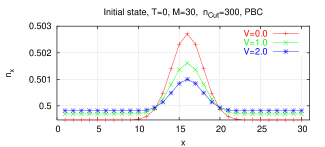
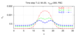
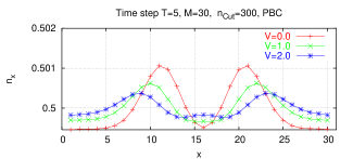
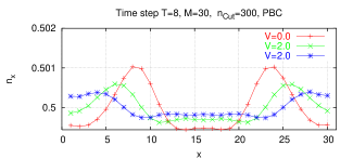
Figure 1: Time evolution of a wave packet for a system of $M=30$ sites, periodic boundary conditions, and $V=0.0$ (plus), $V=1.0$ (crosses) and $V=2.0$ (stars). The snapshots are taken at $T=0$, $2$, $5$, and $8$. $n_{\rm Cut}=300$ states per block were kept within the DMRG procedure.

III Wave packet dynamics

In order to prepare an initial state we apply a small perturbation $\delta{\cal H}$ to the Hamiltonian $\cal H$ of the system of interest and calculate $|{\xi(0)}\rangle$ as the ground state of ${\cal H}+\delta{\cal H}$.

As a first example we study the time evolution of a density pulse in a model of interacting spinless fermions:

$${\cal H}=-t\,\sum_{x=1}^{M}c^{\dagger}_{x}c^{\phantom{\dagger}}_{x-1}+c^{\dagger}_{x-1}c^{\phantom{\dagger}}_{x}\;+\;V\,\sum_{x=1}^{M}\,n_{x}n_{x-1}$$ (6)

where $t$ is the hopping parameter and $V$ the nearest neighbour interaction parameter. In this work we measure all energies with respect to $t=1$. To create a wave packet we add a Gaussian potential

$$\delta{\cal H}=\;-\;\mu\sum_{x=1}^{M}\text{e}^{-\frac{(x-x_{1})^{2}}{2\sigma^{2}}}\,n_{x}$$ (7)

where $\mu$ is the strength, $\sigma$ the width, and $x_{1}$ the position of the perturbation.

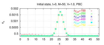
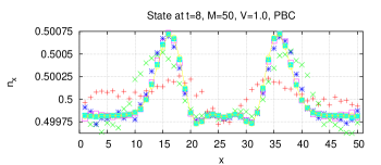
Figure 2: (a) Initial wave packet for a 50 site system with periodic boundary conditions and $V=1$, for different numbers of states kept per block: $n_{\rm Cut}=100$ (plus), $200$ (crosses), $300$ (stars), $400$ (open squares), $500$ (filled squares) and $750$ (open circles). (b) Same system at time $T=8$.

In Fig. (1) we have plotted the time evolution of an initial wave packet at $x_{1}=6$ in a 30 site system at half filling and periodic boundary condition using 300 states per DMRG block. Due to time reversal symmetry the initial state consist of a left and a right moving wave packet. During the time evolution the initial peak splits into two peaks which are moving with the group velocities $\pm v_{g}$. For $V=0$ the DMRG results coincides with the result from exact diagonalization. As a first result this method gives direct access to the group velocity $v_{g}$ of a density excitation without relying on finite size analysis or arguments from conformal field theory.BA:QISM In table (1) we compare the extracted group velocities $v_{g}$ for the $M=30$ site system with the Fermi velocity $v_{F}$ known from Bethe ansatz results for an infinitesimal excitation in the infinite system size limit, $v_{F}=\pi\sin(2\eta)/(\pi-2\eta)$ with the usual parametrization $V=-2\cos(2\eta)$.BA:QISM As expected from $v_{F}$ the wave packets travel faster the stronger repulsive interaction are, while they are slowed down by attractive interaction. For $\mu=0.002$ there is a good agreement from $v_{g}$ with $v_{F}$, while the results for $\mu=0.02$ already include dispersion effects. In addition, the broadening of the wave packets reveals information on the dispersion relation. A detailed study is beyond the scope of this work and subject for future studies.

$U$	-1.5	0.0	0.5	1.0	1.5
$v_{g}$, $\mu=0.02$	1.0	1.9	2.2	2.47	2.71
$v_{g}$, $\mu=0.002$	0.92	2.00	2.30	2.59	2.87
$v_{F}$(BA)	0.88	2.00	2.31	2.60	2.88

Table 1: Comparison of $v_{g}$ extracted from DMRG simulations for a $M=30$ site system and a potential strength $\mu=0.02$ , $\mu=0.002$ and Bethe ansatz results for $v_{F}$ in the infinite system and an infinitesimal small excitation.

It is not obvious that one can target for a few low lying states $|{\Psi_{m}}\rangle$ of $\cal H$, the ground state $\xi(0)$ of ${\cal H}+\delta{\cal H}$ and $N\sim 100$ time steps of $\xi(t_{j})$ simultaneously in each DMRG step. However, since the DMRG truncation is the only approximation in our method, we can systematically increase the number of states $n_{\rm nCut}$ kept per block to control errors due to the Hilbert space truncation. In Fig. (2) we plot an initial wave packet $\xi(0)$ and the wave packet $\xi(T)$ at $T=8$ for a 50 site system, a potential strength of $\mu=0.02$, an interaction strength $V=1.0$ and periodic boundary conditions. While for the initial state 200 states per block seem to be sufficient to describe the wave packet, far more states are needed to obtain the dynamics of the wave packet correctly. The slow convergence at the boundaries of the system is related to an implementation detail. We do not keep all density operators to evaluate $n_{x}$ in the final iteration step. Instead we calculate $n_{x}$ during the last 1.5 finite lattice sweeps, when we have the operators available. The advantage of this procedure is that one does not need to keep all operators at the price that the operators close to boundaries have less accuracy, since they are evaluated in a highly asymmetric block configuration.

Remarkably, the overlap $\langle{\Psi_{0}}|{\xi(0)}\rangle$ between the ground state of $\cal H$ and the ground state of the system of ${\cal H}+\delta{\cal H}$ shown in Fig. (2) is $99.99\%$. Therefore, it is the $0.01\%$ contribution which gives the initial excitation and governs the time evolution. This high overlap was the motivation to introduce the projection defined im Eq. (4).

IV Transport through a quantum dot

In order to study transport through an interacting nano structure, we prepare a system consisting of an interacting region coupled to noninteracting leads, see Fig. (3),

$${\cal H} = -t\,\sum_{x=1}^{M}\left(c^{\dagger}_{x}c^{\phantom{\dagger}}_{x-1}+c^{\dagger}_{x-1}c^{\phantom{\dagger}}_{x}\right)\;+\;U\,\sum_{x=n_{1}+1}^{n_{2}-1}\,n_{x}n_{x-1}$$ (8)

$$\;+\;\gamma\,U\,\sum_{x=n_{1},n_{2}}\,n_{x}n_{x-1}\,,$$

where $t$ is hopping parameter, $U$ is the interaction on the nano structure and $\gamma$ defines a smoothening of the onset of interaction at the nano structure. In this work we have set $\gamma=0.5$, compare Molina et al. DMRG:PC-Molina . In the following we denote $M_{S}=n_{2}-n_{1}$ the number of sites in the nano structure, $M$ the number of site of the total system and $M_{L}=M-M_{S}$ the number of lead sites.

In Fig. (4) we show the time evolution of a wave packet initially placed in the left lead of a system with $M_{S}=7$, $M=50$, interaction $V=0.0$, $1.0$, $2.0$ and $5.0$ and hard wall boundary conditions, which lead to perfect reflection at the chain ends. To rule out truncation errors we use $n_{\rm Cut}=1000$ states per block, compare discussion of Fig. (2). We have averaged the density over neighbouring sites to smoothen out the Friedel oscillations (for all $V$) and the charge density wave on the dot for $V=5.0$. At the beginning of the time evolution, the wave packet is not overlapping with the interacting nano structure, hence the packets travel synchronously for all interaction strength. Once they reach the nano structure, the wave packets move with the group velocity of the interacting system. After the wave packets have left the interacting region they continue to move at the velocity of the noninteracting system. The wave packets which traveled through the interacting region are now travelling in front of those with smaller interaction.

For $U<=2.0$ the nano structure is transparent, although there seems to be a reflection of a negative pulse as predicted by Safi and Schulz Safi95 . For very strong interaction, $U>2.0$, there is an instability to a charge density ordering,DMRG:MUS ; BA:QISM and the nano structure has a finite reflection. We would like to remark that these simulations clearly demonstrate that the Luttinger description of the infinite system makes already sense for a system consisting of a few lattice sites only. One should should keep in mind that for such small systems the effective parameters, like $v_{F}$, have not reached the infinite system limit. However, the scaling already leaves its fingerprint.

Figure 3: Nano structure attached to leads.

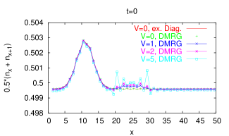
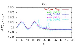
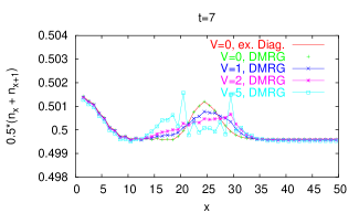
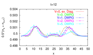
Figure 4: Transport through an interacting region of $M_{S}=7$ sites and $M_{L}=43$ lead sites, hard wall boundary conditions and $n_{\rm Cut}=1000$. The snapshots are taken at $T=0$, $3$, $7$, $12$. The density is averaged over 2 neighbouring site to smoothen $2k_{F}$ oscillations and is plotted vs. the site location $x$ for $V=0$ (plus), $V=1$ (crosses), $V=2$ stars, and $V=5$ (squares). For $V=0$ the line is calculated by an exact diagonalization.

V Summary

In summary we have shown an accurate method to calculate real time dynamics within the framework of DMRG. By applying the matrix exponential on our initial state state we are able to perform the complete time integration of the time dependent Schrödinger equation in each single DMRG step. In this setup the only approximation is given by the truncation procedure of the DMRG, which be can systematically checked by increasing the number of states kept during the DMRG sweeps.

VI Note

While preparing this work we became aware of related work TdDMRG:White ; TdDMRG:Schollwoeck on using real time dynamics within the DMRG. Both apply a Suzuki-Trotter decomposition of the time evolution operator, based on an work by by Vidal.Vidal03 In addition, their work relies on the state prediction DMRG:WhitePrediction to calculate the time evolution of a state, which represents an additional approximation. In contrast to their work we calculate the initial state and apply the full time evolution operator in each iteration step, without introducing additional approximations beyond the truncation scheme of the DMRG.

VII Acknowledgement

I acknowledge the support of the Center for Functional Nano Structures within project B2.10. I would like to thank Karl Meerbergen for his hints on the matrix exponential and insightful discussions with Ralph Werner, Peter Wölfle and Gert L. Ingold.

References

- (1) S. R. White , Phys. Rev. Lett. 69, 2863 (1992) ; Phys. Rev. B 48, 10345 (1993).
- (2) Density Matrix Renormalization – A New Numerical Method in Physics, edited by I. Peschel, X. Wang, M.Kaulke, and K. Hallberg (Springer, Berlin, 1999).
- (3) P. Schmitteckert, T. Schulze, C. Schuster, P. Schwab, and U. Eckern Phys. Rev. Lett. 80, 560 (1998); D. Weinmann, J. L. Pichard, P. Schmitteckert, and R. A. Jalabert, Phys. Rev. Lett. 81, 2308 (1998).
- (4) P. Schmitteckert and R. Werner, accepted by Phys. Rev. B (2004).
- (5) K. A. Hallberg , Phys. Rev. B 52, 9827 (1995).
- (6) T. D. Kühner and S. R. White , Phys. Rev. B 60, 335 (1999).
- (7) E. Jeckelmann Phys. Rev. B 66, 045114 (2002).
- (8) R. A. Molina, D. Weinmann, R. A. Jalabert, G.-L. Ingold, J.-L. Pichard, Phys. Rev. B 67, 235306 (2003).
- (9) V. Meden, U. Schollwöck, Phys. Rev. B 67, 193303 (2003).
- (10) O. P. Sushkov, Phys. Rev. B 64, 155319 (2001).
- (11) M. A. Cazalilla and J. B. Marston , Phys. Rev. Lett. 88, 256403 (2002).
- (12) H. G. Luo, T. Xiang, and X. Q. Wang , Phys. Rev. Lett. 91, 049701 (2003).
- (13) Y. Saad, SIAM J. Numer. Anal. 29 (1998), 130.
- (14) C. Moler and C. Van Loan, SIAM Review 45 (2003), No. 1, 3.
- (15) R. B. Sidje, ACM Trans. Math. Software, 24 (1998), 130; R. B. Sidje, Expokit software, ACM - TOMS, 24(1):130-156, (1998).
- (16) Additional states are needed for the calculation of the Krylov subspace.
- (17) V. E. Korepin, N. M. Bogoliubov, and A. G. Izergin, Quantum Inverse Scattering Method and Correlation Functions (Cambridge University Press, Cambridge, 1993).
- (18) I. Safi and H. H. Schultz in Quantum Transport in Semiconductor Submicron Structures , edited by B. Kramer, Kluwer Academic Press, AA Dordrecht (1995).
- (19) S. R. White and A. E. Feiguin, cond-mat/0403310.
- (20) A. J. Daley, C. Kollath, U. Schollwoeck , and G. Vidal., cond-mat/0403313.
- (21) G. Vidal, Phys. Rev. Lett. 91 (2003), 147902.
- (22) S. R. White, Phys. Rev. Lett. 77, 3633 (1996).