Spanning avalanches in the three-dimensional Gaussian Random Field Ising Model with metastable dynamics: field dependence and geometrical properties

Abstract

Spanning avalanches in the 3D Gaussian Random Field Ising Model (3D-GRFIM) with metastable dynamics at $T=0$ have been studied. Statistical analysis of the field values for which avalanches occur has enabled a Finite-Size Scaling (FSS) study of the avalanche density to be performed. Furthermore, direct measurement of the geometrical properties of the avalanches has confirmed an earlier hypothesis that several kinds of spanning avalanches with two different fractal dimensions coexist at the critical point. We finally compare the phase diagram of the 3D-GRFIM with metastable dynamics with the same model in equilibrium at $T=0$.

I Introduction

Avalanche behavior J.P.Sethna et al. (2001) has been found in many first order phase transitions at low temperatures. When the external parameters are slowly driven, the transition, instead of occurring as a sharp change of the system properties at a certain point of the phase diagram, splits into a series of discontinuous jumps that link metastable states. This gives rise to hysteresis loops, whose branches consist of a sequence of random steps. In many cases the sizes of such steps range from microscopic to macroscopic scales, distributed according to a power-law. The phenomenon has been found to be associated with magnetic transitions Babcock and Westervelt (1990); P.J.Cote and L.V.Meisel (1991); Puppin (2000), capillary condensation M.P.Lilly et al. (1993); E.Kierlik et al. (2001), martensitic transformations Vives et al. (1994), and others Casanova et al. . A crucial ingredient in order to observe such avalanches is that thermal fluctuations are very small compared with the energy barriers that separate transformed and untransformed domains. For this reason, such first-order phase transitions have been called “athermal” F.J.Pérez-Reche et al. (2001) or “fluctuationless” Vives and Planes (1994); Carrillo et al. (1998).

Within this context the 3D-GRFIM with metastable dynamics is a prototype model: the complexity of what we call “disorder” in a real system is simplified into a series of quenched random fields, Gaussian distributed with zero mean and standard deviation $\sigma$, that act on every spin of a 3D Ising model. In addition, one assumes that temperature is zero ($T=0$) and provides the model with a particular metastable dynamics in order to study the evolution of the magnetization $m$ when the external field $H$ is swept. The details of the dynamics were introduced by Sethna and coworkers a decade ago Sethna et al. (1993); Dahmen and J.P.Sethna (1993). The basic assumption is that the driving field rate is slow enough so that system relaxation can be considered instantaneous (adiabatic driving). Such relaxations are the so-called magnetization avalanches.

After the introduction of the model several works Perković et al. (1995); Dahmen and J.P.Sethna (1996); Tadić (1996); Perković et al. (1999); Kuntz et al. (1999); J.H.Carpenter and K.A.Dahmen (2002) described the basic associated phenomenology: (a) the existence of a disorder-induced critical point at $\sigma=\sigma_{c}$ associated with the change from a continuous to a discontinuous hysteresis loop and (b) the fact that within a large region around the critical point the distribution of avalanche sizes $D(s)$ exhibits almost power-law behavior. Nevertheless, several questions remain unsolved, mostly related to the properties of the spanning avalanches which are responsible for the observed macroscopic discontinuities in the $H$-$m$ hysteresis loop and in the $\sigma$-$H$ phase diagram.

More recently, a FSS analysis of the number of avalanches and avalanche size distribution Pérez-Reche and Vives (2003) has revealed that the scenario is quite complex. The study was restricted to the statistical analysis of the full set of avalanches recorded in a half loop, irrespective of the field values $H$ where such avalanches occur. (The obtained statistical distributions are often called integrated distributions). A detailed study as a function of $H$ has not been done before.

Let us summarize here the main results presented in Ref. Pérez-Reche and Vives (2003), in order to introduce the notation. According to the dependence on the system size $L$ of the average number $N_{\alpha}(\sigma,L)$ and size distribution $D_{\alpha}(s;\sigma,L)$, avalanches can be classified into several categories, (the subindex $\alpha$ stands for the different categories) as presented in Table 1. The scaling behavior is written as a function of the variable $u$ which measures the distance to the critical value of the disorder $\sigma_{c}=2.21\pm 0.02$. Its precise definition is given as a second-order expansion:

$$u=\frac{\sigma-\sigma_{c}}{\sigma_{c}}+A\left(\frac{\sigma-\sigma_{c}}{\sigma_{c}}\right)^{2}$$ (1)

with $A=-0.2$. This expression was found to be the best choice for the collapse of the scaling plots. The values of the different critical exponents are summarized in Table 2, together with the new exponents that will be computed in the present work.

avalanche type	$\alpha$	average number	size distribution
non-spanning	$ns$	$N_{ns}(\sigma,L)\;\;\;\left[N_{ns}=N_{nsc}+N_{ns0}\right]$	$D_{ns}(s;\sigma,L)\;\;\;\left[N_{ns}D_{ns}=N_{nsc}D_{nsc}+N_{ns0}D_{ns0}\right]$
critical non-spanning	$nsc$	$N_{nsc}(\sigma,L)=L^{\theta_{nsc}}\tilde{N}_{nsc}(uL^{1/\nu})$	$D_{nsc}(s;\sigma,L)=L^{-\tau_{nsc}d_{f}}\tilde{D}_{3c}(sL^{-d_{f}},uL^{1/\nu})$
non-critical non-spanning	$ns0$	$N_{ns0}(\sigma,L)=L^{3}\tilde{N}_{ns0}(\sigma)$
1D-spanning	1	$N_{1}(\sigma,L)=L^{\theta}\tilde{N}_{1}(uL^{1/\nu})$	$D_{1}(s;\sigma,L)=L^{-d_{f}}\tilde{D}_{1}(sL^{-d_{f}},uL^{1/\nu})$
2D-spanning	2	$N_{2}(\sigma,L)=L^{\theta}\tilde{N}_{2}(uL^{1/\nu})$	$D_{2}(s;\sigma,L)=L^{-d_{f}}\tilde{D}_{2}(sL^{-d_{f}},uL^{1/\nu})$
3D-spanning	3	$N_{3}(\sigma,L)\;\;\;\left[N_{3}=N_{3c}+N_{3-}\right]$	$D_{3}(s;\sigma,L)\;\;\;\left[N_{3}D_{3}=N_{3c}D_{3c}+N_{3-}D_{3-}\right]$
critical 3D-spanning	3$c$	$N_{3c}(\sigma,L)=L^{\theta}\tilde{N}_{3c}(uL^{1/\nu})$	$D_{3c}(s;\sigma,L)=L^{-d_{f}}\tilde{D}_{3c}(sL^{-d_{f}},uL^{1/\nu})$
subcritical 3D-spanning	3-	$N_{3-}(\sigma,L)=\tilde{N}_{3-}(uL^{1/\nu})$	$D_{3-}(s;\sigma,L)=L^{-d_{3-}}\tilde{D}_{3-}(sL^{-d_{3-}},uL^{1/\nu})$

Table 1: Classification of the different types of avalanches in the 3D-RFIM according to their geometrical properties and their finite-size scaling behavior. Non-spanning avalanches and 3D-spanning avalanches exhibit mixed scaling behavior (indicated in square brackets). They can be separated into two subcategories.

exponent	best value	Ref
$\nu$	$1.2\pm 0.1$	Pérez-Reche and Vives,2003
$\theta$	$0.10\pm 0.02$	Pérez-Reche and Vives,2003
$\theta_{nsc}$	$2.02\pm 0.04$	Pérez-Reche and Vives,2003
$d_{f}$	$2.78\pm 0.05$	Pérez-Reche and Vives, 2003, this work
$d_{3-}$	$2.98\pm 0.02$	Pérez-Reche and Vives, 2003, this work
$\tau_{nsc}$	$1.65\pm 0.02$	Pérez-Reche and Vives,2003
$\beta_{c}$	$0.15\pm 0.08$	Pérez-Reche and Vives,2003
$\beta_{3-}$	$0.024\pm 0.012$	Pérez-Reche and Vives,2003
$1/\mu$	$1.5\pm 0.1$	this work

Table 2: Summary of the values of the critical exponents of the 3D-GRFIM with metastable dynamics, obtained in Ref. Pérez-Reche and Vives, 2003 and in the present work, as indicated in the last column.

Classification of the avalanches starts by checking whether the avalanches span the system in 1,2 or 3 spatial directions. These three kinds of spanning avalanches are indicated by $\alpha=1,2,3$ respectively.

To obtain good scaling collapses of the 3D-spanning avalanches, an extra hypothesis was introduced: they can be separated into two subcategories, subcritical ($\alpha=3-$) and critical ($\alpha=3c$) that scale with different exponents. In particular, this assumption indirectly leads to the conclusion that they must have different fractal dimensions $d_{3-}$ and $d_{f}$. Moreover, non-spanning avalanches ($\alpha=ns$) should also be separated into two subcategories: non critical ($\alpha=ns0$) and critical ($\alpha=nsc$), depending on whether their number and size distribution scales with distance to the critical point $u$ or not.

Fig. 1 presents a summary Vives and Pérez-Reche (2004) of the scaling functions $\tilde{N}_{\alpha}$ according to the results in Ref. Pérez-Reche and Vives (2003). From the behavior of such scaling functions when $uL^{1/\nu}\rightarrow\pm\infty$ one can sketch out the scenario in the thermodynamic limit. Below $\sigma_{c}$ one subcritical 3D-spanning avalanche exists, which is responsible for the observed discontinuity of the magnetization in the thermodynamic limit. Such a discontinuity is the order parameter and vanishes when approaching $\sigma_{c}^{-}$ according to $\Delta m\propto(\sigma_{c}-\sigma)^{\beta_{3-}}$, with an exponent $\beta_{3-}=\nu(3-d_{3-})=0.024\pm 0.012$. Nevertheless, it is difficult to find this critical behavior from simulations of finite systems since the contributions from critical spanning avalanches ($\alpha=1$,$2$ and $3c$) may lead to quite good (but incorrect) scaling collapses of the order parameter using $\beta_{c}=\nu(3-\theta-df)=0.15\pm 0.08$.

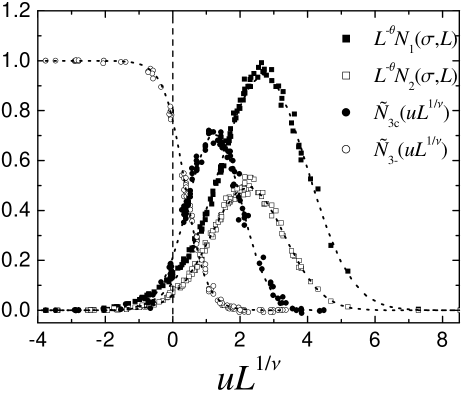
Figure 1: Scaling functions corresponding to the number of 1D-, 2D-, critical 3D- and subcritical 3D-spanning avalanches in the 3D-RFIM as found in Ref. Pérez-Reche and Vives (2003). The symbols show the overlap of the data corresponding to numerical simulations with many different system sizes ranging from $L=5$ to $L=48$.

A large number of non-critical non-spanning avalanches exist for the whole range of $\sigma$. They cannot contribute to any observed macroscopic jump since their size is vanishingly small in the thermodynamic limit. At $\sigma=\sigma_{c}$ the 6 categories of avalanches exist. On average, one finds $0.79\pm 0.02$ subcritical 3D-spanning avalanches and an infinite number of the five other types of avalanches. At the critical point (or close enough to it), the distribution of avalanche sizes is dominated by critical non-spanning avalanches and exhibits an approximate power-law behavior with an exponent $\tau_{eff}=\tau_{nsc}+(3-\theta_{nsc})/d_{f}=2.00\pm 0.06$. This power law behavior is restricted to the central part of the avalanche size distribution $1\ll s\ll L^{3}$.

In the present paper we will concentrate on the 4 different kinds of spanning avalanches, extending the finite-size scaling analysis and focusing on (i) the study of the values of the external field for which the spanning avalanches occur and (ii) the direct measurement of the geometrical properties of the avalanches. This will enable the critical exponent $\mu$, related to the renormalization group (RG) flow along the field direction, to be found and have a direct test of the FSS hypothesis that leads to the separation of the two kinds of 3D-spanning avalanches (critical and subcritical) with different fractal dimensions: $d_{f}=2.78\pm 0.05$ and $d_{3-}=2.98\pm 0.02$.

In section II we summarize the 3D-GRFIM and the details of our numerical simulations. In section III raw numerical results are presented. In section IV we discuss the main FSS hypothesis, as an extension of those presented previously. These hypotheses are checked in section V. In section VI we determine the geometrical properties of the avalanches. In section VII we discuss the consequences of the present study and, finally, in section VIII we summarize and conclude our findings.

II Model

The 3D-GRFIM is defined on a cubic lattice of size $L\times L\times L$ with periodic boundary conditions. On each lattice site ($i=1,\dots,L^{3}$) there is a spin variable $S_{i}$ taking values $\pm 1$. The Hamiltonian is:

$${\cal H}=-\sum_{i,j}^{n.n.}S_{i}S_{j}-\sum_{i=1}^{L^{3}}h_{i}S_{i}-H\sum_{i=1}^{L^{3}}S_{i}\;\;,$$ (2)

where the first sum extends over all nearest-neighbor (n.n) pairs, $H$ is the external applied field and $h_{i}$ are quenched random fields, which are independent and are distributed according to a Gaussian probability density with zero mean and standard deviation $\sigma$.

The equilibrium ground-state ($T=0$) of this Hamiltonian has been recently studied Middleton and D.S.Fisher (2002). In this work we focus on the metastable version of the 3D-GRFIM proposed for the analysis of the behavior at $T=0$ when the system is driven by the external field $H$. For $H=+\infty$ the state of the system which minimizes $\cal H$ is the state with maximum magnetization $m=\sum_{i=1}^{L^{3}}S_{i}/L^{3}=1$. When the external field $H$ is decreased, the system evolves following local relaxation dynamics. The spins flip according to the sign of the local field:

$$h_{i}+H+\sum_{j=1}^{6}S_{j}\;\;,$$ (3)

where the sum extends over the 6 nearest-neighboring spins of $s_{i}$. Avalanches occur when a spin flip changes the sign of the local field of some of the neighbors. This may start a sequence of spin flips which occur at a fixed value of the external field $H$, until a new stable situation is reached. $H$ is then decreased again. The size of the avalanche $s$ corresponds to the number of spins flipped until a new stable situation is reached. Note that the corresponding magnetization change is $\Delta m=2s/L^{3}$.

The numerical algorithm we have used is the so-called brute force algorithm which propagates one avalanche at a time Kuntz et al. (1999). We have studied system sizes ranging from $L=5(L^{3}=125)$ to $L=180(L^{3}=5832000)$. The measured properties are always averaged over a large number of realizations of the random field configuration for each value of $\sigma$, which ranges between more than $10^{4}$ for $L\leq 80$ to $300$ for $L=180$.

We have recorded the sequence of avalanche sizes during half a hysteresis loop, i.e. decreasing $H$ from $+\infty$ to $-\infty$. We have determined not only the size $s$ of each individual avalanche, but also the field $H$ at which each avalanche occurs. The avalanches have been classified as non-spanning, 1D-spanning, 2D-spanning and 3D-spanning as explained in Ref. Pérez-Reche and Vives (2003).

By performing statistics, we obtain the average density of avalanches for each type occurring within an interval $(H,H+dH)$ . We will call this quantity the number density $n_{\alpha}(H;\sigma,L)$. It satisfies:

$$\int_{-\infty}^{\infty}dH\;n_{\alpha}(H;\sigma,L)=N_{\alpha}(\sigma,L)$$ (4)

where $N_{\alpha}(\sigma,L)$ are the average number of avalanches of each kind Pérez-Reche and Vives (2003) defined in Table 1. We have also measured the bivariate size distribution ${\cal D}_{\alpha}(s,H;\sigma,L)$. This probability density is normalized so that:

$$\sum_{s=1}^{L^{3}}\int_{-\infty}^{\infty}dH\;{\cal D}_{\alpha}(s,H;\sigma,L)=1$$ (5)

Note that by projecting ${\cal D}_{\alpha}$ we can obtain the two marginal distributions:

$$\sum_{s=1}^{L^{3}}{\cal D}_{\alpha}(s,H;\sigma,L)=\frac{n_{\alpha}(H;\sigma,L)}{N_{\alpha}(\sigma,L)}$$ (6)

and

$$\int_{-\infty}^{\infty}dH\;{\cal D}_{\alpha}(s,H;\sigma,L)=D_{\alpha}(s;\sigma,L)$$ (7)

which represent the probability density of finding an avalanche of type $\alpha$ within $(H,H+dH)$ and the probability (integrated distribution) that an avalanche of type $\alpha$ has a size $s$ (after the half loop) respectively.

In the following sections bivariate distributions will be presented as point clouds and the marginal distributions as histograms. Point clouds provide qualitative understanding of the distributions. Quantitative analysis is much better performed from the marginal distributions and their moments. The average field where the different types of avalanches occur will be particularly interesting:

$$\langle H\rangle_{\alpha}(\sigma,L)=\int_{-\infty}^{\infty}dH\;H\frac{n_{\alpha}(H;\sigma,L)}{N_{\alpha}(\sigma,L)},$$ (8)

and its standard deviation:

$$\sigma_{\alpha}^{H}(\sigma,L)=\left(\langle H^{2}\rangle_{\alpha}-\langle H\rangle_{\alpha}^{2}\right)^{1/2}.$$ (9)

In some simulations we have also performed a sand box counting analysis Bunde and Havlin (1994) of each individual spanning avalanche in order to have a direct determination of their fractal dimension. The method consists of considering boxes of linear size $\ell$ (ranging from $1\times 1\times 1$, $3\times 3\times 3$, $5\times 5\times 5$, … up to $(L-1)\times(L-1)\times(L-1)$) centred near the spin that triggered each spanning avalanche. We determine the number of sites that belong to the avalanche for each box. By averaging over all the avalanches of the same kind (occurring during a half loop) and over many disorder realizations, we obtain the mass $M_{\alpha}(\ell;\sigma,L)$ as a function of the box length $\ell$.

III Numerical results

Fig. 2 shows a point cloud corresponding to ${\cal D}_{3}(s,H;\sigma,L)$ for $L=48$ and different values of $\sigma$. As can be seen, below $\sigma_{c}$ 3D-spanning avalanches are large, close to $s=L^{3}$ and exhibit a certain spread around a value of $H$ which shifts upwards when $\sigma_{c}$ is approached from below. At $\sigma=\sigma_{c}$ the avalanches concentrate around a critical field value $H_{c}\simeq-1.42$ and span almost all possible sizes. Above $\sigma_{c}$ the few existing 3D-spanning avalanches are small. In fact, they are smaller than the mean size of a percolating cluster in a 3D cubic lattice ($s=0.311L^{3}$).

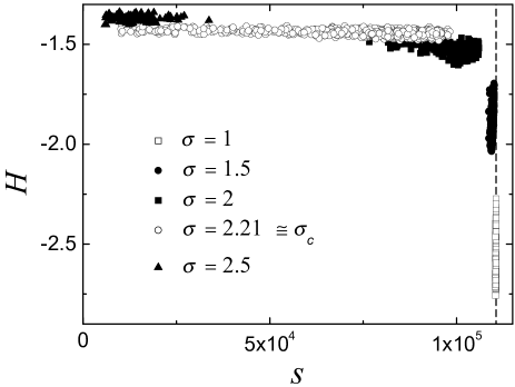
Figure 2: Point clouds corresponding to 3D-spanning avalanches for a system with size $L=48$. Each point corresponds to an individual avalanche and indicates the size $s$ and the field where it occurred $H$. Clouds corresponding to different values of $\sigma$ are indicated by different symbols. Data have been averaged over many realizations of disorder. The dashed line indicates the maximum value $s=L^{3}$.

Fig. 3 shows the point clouds corresponding to non-spanning, 1D-, 2D-, and 3D-spanning avalanches at $\sigma=\sigma_{c}$. Non-spanning avalanches are suppressed from the main plot, but are shown in the inset on a log-linear scale. As expected, spanning avalanches concentrate around $H_{c}$. 3D-spanning avalanches exhibit a larger size than 2D-spanning avalanches and the latter show a size larger than 1D-spanning avalanches. Moreover, one can see that 3D-spanning avalanches are distributed in a double cloud. As will be seen, these two clouds correspond to the two types of 3D-spanning avalanches predicted in Pérez-Reche and Vives (2003).

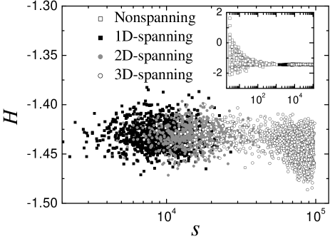
Figure 3: Point clouds corresponding to 1D-, 2D-, and 3D-spanning avalanches at $\sigma=\sigma_{c}$ for $L=48$. The inset shows, on a log-linear scale, the same data together with the cloud corresponding to non-spanning avalanches.

The dependence on the system size $L$ is illustrated in Fig. 4. The point clouds represent the distribution of spanning avalanches at $\sigma=\sigma_{c}$ for increasing values of $L$. The three plots correspond to (a) 1D-, (b) 2D-, and (c) 3D-spanning avalanches. The dashed line corresponds to our estimated value of $H_{c}=-1.425$. Note that all kinds of spanning avalanches tend to concentrate around such a field value for increasing system sizes. The shape of the cloud corresponding to 3D-spanning avalanches remains assymetric, while $L$ grows.

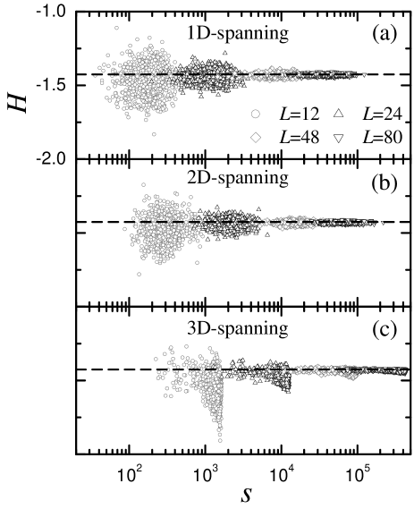
Figure 4: Point clouds corresponding to 1D- (a), 2D- (b) and 3D-spanning avalanches (c) at $\sigma=\sigma_{c}$ for increasing system sizes, as indicated by the legend. The same scale is used on the three plots.

To obtain a quantitative measure of $H_{c}$, we have computed the field averages $\langle H\rangle_{1}$, $\langle H\rangle_{2}$ and $\langle H\rangle_{3}$. Their behavior as a function of $L$ at $\sigma=\sigma_{c}$ is plotted in Fig. 5(a). In the next sections a FSS analysis will be formally proposed. Nevertheless, from the behavior in Fig. 5(a) one can already guess the following scaling hypothesis:

$$\langle H\rangle_{\alpha}(\sigma_{c},L)-H_{c}\sim C_{\alpha}L^{1/\mu},$$ (10)

where $\mu$ will be the exponent governing the divergence of the correlation length when the field $H$ approaches $H_{c}$ at $\sigma=\sigma_{c}$. A first check of this hypothesis is performed in Fig. 5(b) by a 3-parameter ($H_{c}$, $\mu$ and $C_{\alpha}$) least-squares fit to the three sets of data. We have obtained the same values of $1/\mu=1.5\pm 0.1$ and $H_{c}=-1.425\pm 0.010$ for $\langle H\rangle_{1}$, $\langle H\rangle_{2}$ and $\langle H\rangle_{3}$. Results of the fits are indicated by dotted lines in Figs. 5(a) and 5(b).

Figure 5: (a) Average fields $\langle H\rangle_{\alpha}(\sigma_{c},L)$. The dashed lines indicates $H_{c}=-1.425$ and the dotted lines correspond to power-law fits. (b) The same data represented on log-log scales. The lines indicates the power-law behavior. Note that the 3 kinds of spanning avalanches exhibit the same exponent.

IV Finite-Size Scaling hypothesis

IV.1 Scaling of distributions

To proceed with the analysis of the numerical data one must postulate the ad-hoc FSS hypothesis. As done in Ref. Pérez-Reche and Vives (2003), we follow standard RG arguments. The distance to the critical point $(\sigma_{c},H_{c})$ is measured with two scaling variables $u(\sigma,H)$ and $v(\sigma,H)$, which depend on the externally tunable parameters $\sigma$ and $H$. After a renormalization step that transforms the system size $L$ as:

$$L_{b}=b^{-1}L.$$ (11)

$u$,$v$, and the size $s$ of an avalanche of type $\alpha$ will behave as:

$$u_{b}=b^{1/\nu}u\;\;\;\;\;v_{b}=b^{1/\mu}v\;\;\;\;\;s_{b}=b^{-d_{\alpha}}s,$$ (12)

where $d_{\alpha}$ are the fractal dimensions of the avalanches and the exponents $\nu$ and $\mu$ control the divergence of the correlation length when approaching the critical point along the two directions $u$ and $v$. Consequently, in order to formulate the FSS hypothesis, we will consider the following three main RG invariants:

$$uL^{1/\nu}=u_{b}L_{b}^{1/\nu}$$ (13)

$$vL^{1/\mu}=v_{b}L_{b}^{1/\mu}$$ (14)

$$sL^{-d_{\alpha}}=s_{b}L_{b}^{-d_{\alpha}}$$ (15)

Therefore, close enough to the critical point the bivariate distributions ${\cal D}_{\alpha}(s,H;\sigma,L)$ will behave as:

$${\cal D}_{\alpha}(s,H;\sigma,L)=L^{-{d_{\alpha}}+1/\mu}\hat{\cal{D}}_{\alpha}\left(sL^{-d_{\alpha}},uL^{1/\nu},vL^{1/\mu}\right)$$ (16)

where $d_{\alpha}$ is $d_{f}=2.78$ for the 1D-,2D- and critical 3D-spanning avalanches and $d_{3-}=2.98$ for the subcritical 3D-spanning avalanches, as found in Ref. Pérez-Reche and Vives (2003).

The number densities $n_{\alpha}(H;\sigma,L)$ will behave as:

$$n_{\alpha}(H;\sigma,L)=L^{\theta_{\alpha}+1/\mu}{\hat{n}}_{\alpha}\left(uL^{1/\nu},vL^{1/\mu}\right),$$ (17)

where $\theta_{\alpha}$ is $\theta_{c}=0.1$ for the 1D-, 2D- and critical 3D-spanning avalanches and $\theta_{\alpha}=0$ for the subcritical 3D-spanning avalanches. The FSS hypothesis (16) and (17) extend the hypothesis presented in Table 1, including the dependence on the external field $H$.

IV.2 Detailed scaling variables

The proper dependence of the scaling variables $u$ and $v$ on the tunable model parameters $\sigma$ and $H$ is unknown, but it should be analytic S.K.Ma (1973); J.Cardy (1996). Keeping this in mind, we consider the following second-order expansion around $\sigma=\sigma_{c}$ and $H=H_{c}$:

$$u = u_{1}+Au_{1}^{2}+A^{\prime}v_{1}+A^{\prime\prime}u_{1}v_{1}+A^{\prime\prime\prime}v_{1}^{2}$$ (18)

$$v = v_{1}+Bv_{1}^{2}+B^{\prime}u_{1}+B^{\prime\prime}u_{1}v_{1}+B^{\prime\prime\prime}u_{1}^{2},$$ (19)

where $u_{1}=(\sigma-\sigma_{c})/\sigma_{c}$ and $v_{1}=(H-H_{c})/H_{c}$ are the first-order scaling variables. These variables represent the simplest choice to measure the distance to the critical point. Now we want to check which corrections to the first-order scaling variables are really important for large system sizes. Consider a function $F(H;\sigma,L)$ that can be written as

$$F(H;\sigma,L)=L^{a}\hat{F}(uL^{1/\nu},vL^{1/\mu}),$$ (20)

when the correct scaling variables are considered. In the case in which we try to obtain scaling collapses with two incorrect scaling variables $u^{\prime}$ and $v^{\prime}$, an explicit dependence on $L$ may appear, which makes the collapse $L^{-a}F$ impossible for different system sizes. In such a situation:

$$F(H;\sigma,L)=L^{a}\hat{G}(u^{\prime}L^{1/\nu},v^{\prime}L^{1/\mu},L),$$ (21)

where we have introduced a “non”-scaling function $\hat{G}$ that depends explicitly on $L$. By construction, $\hat{G}$ coincides with $\hat{F}(uL^{1/\nu},vL^{1/\mu})$ when $u^{\prime}=u$ and $v^{\prime}=v$. The effective scaling variables $u^{\prime}$ and $v^{\prime}$ can be expanded up to second order:

$$u^{\prime} = u_{1}+{\cal A}u_{1}^{2}+{\cal A}^{\prime}v_{1}+{\cal A}^{\prime\prime}u_{1}v_{1}+{\cal A}^{\prime\prime\prime}v_{1}^{2}$$ (22)

$$v^{\prime} = v_{1}+{\cal B}v_{1}^{2}+{\cal B}^{\prime}u_{1}+{\cal B}^{\prime\prime}u_{1}v_{1}+{\cal B}^{\prime\prime\prime}u_{1}^{2}.$$ (23)

Up to second order, the difference between $\hat{G}(u^{\prime}L^{1/\nu},v^{\prime}L^{1/\mu},L)$ and $\hat{F}(uL^{1/\nu},vL^{1/\mu})$ is

$$\hat{G}(u^{\prime}L^{1/\nu},v^{\prime}L^{1/\mu},L)-\hat{F}(uL^{1/\nu},vL^{1/\mu})=$$ (24)

$$L^{1/\nu}\hat{F}_{1}(uL^{1/\nu},vL^{1/\mu})(u^{\prime}-u)$$

$$+ L^{1/\mu}\hat{F}_{2}(uL^{1/\nu},vL^{1/\mu})(v^{\prime}-v)$$

$$+ \frac{1}{2}L^{2/\nu}\hat{F}_{11}(uL^{1/\nu},vL^{1/\mu})(u^{\prime}-u)^{2}$$

$$+ \frac{1}{2}L^{2/\mu}\hat{F}_{22}(uL^{1/\nu},vL^{1/\mu})(v^{\prime}-v)^{2}$$

$$+ L^{1/\nu+1/\mu}\hat{F}_{12}(uL^{1/\nu},vL^{1/\mu})(u^{\prime}-u)(v^{\prime}-v),$$

where the subindex 1 and 2 in the scaling functions $\hat{F}$ indicate the partial derivatives with respect to $uL^{1/\nu}$ and $vL^{1/\mu}$, respectively. Introducing the expansions (18), (19), (22), and (23) in Eq. (24), defining an appropriate set of eleven functions $\hat{f}_{i}(u_{1}L^{1/\nu},v_{1}L^{1/\mu})$ from the derivatives of $\hat{F}$, and re-ordering the terms in (24) we can write:

$$\hat{G}(u^{\prime}L^{1/\nu},v^{\prime}L^{1/\mu},L)-\hat{F}(uL^{1/\nu},vL^{1/\mu})=({\cal A}^{\prime}-A^{\prime})L^{1/\nu-1/\mu}\left(\frac{v_{1}}{v}\right)\hat{f}_{1}+({\cal B}^{\prime}-B^{\prime})L^{1/\mu-1/\nu}\left(\frac{u_{1}}{u}\right)\hat{f}_{2}$$ (25)

$$+ ({\cal A}-A)L^{-1/\nu}\left(\frac{u_{1}}{u}\right)^{2}\hat{f}_{3}+({\cal B}-B)L^{-1/\mu}\left(\frac{v_{1}}{v}\right)^{2}\hat{f}_{4}$$

$$+ ({\cal A}^{\prime\prime}-A^{\prime\prime})L^{-1/\mu}\left(\frac{u_{1}}{u}\right)\left(\frac{v_{1}}{v}\right)\hat{f}_{5}+({\cal B}^{\prime\prime}-B^{\prime\prime})L^{-1/\nu}\left(\frac{u_{1}}{u}\right)\left(\frac{v_{1}}{v}\right)\hat{f}_{6}$$

$$+ ({\cal A}^{\prime\prime\prime}-A^{\prime\prime\prime})L^{1/\nu-2/\mu}\left(\frac{v_{1}}{v}\right)^{2}\hat{f}_{7}+({\cal B}^{\prime\prime\prime}-B^{\prime\prime\prime})L^{1/\mu-2/\nu}\left(\frac{u_{1}}{u}\right)^{2}\hat{f}_{8}$$

$$+ ({\cal A}^{\prime}-A^{\prime})^{2}L^{2/\nu-2/\mu}\left(\frac{v_{1}}{v}\right)^{2}\hat{f}_{9}+({\cal B}^{\prime}-B^{\prime})^{2}L^{2/\mu-2/\nu}\left(\frac{u_{1}}{u}\right)^{2}\hat{f}_{10}$$

$$+ ({\cal A}^{\prime}-A^{\prime})({\cal B}^{\prime}-B^{\prime})\left(\frac{u_{1}}{u}\right)\left(\frac{v_{1}}{v}\right)\hat{f}_{11},$$

where the dependence of the functions $\hat{f}_{i}$ on $u_{1}L^{1/\nu}$ and $v_{1}L^{1/\mu}$ is not written for simplicity.

Given that $1/\nu=0.8$ (Table 2) and $1/\mu=1.5$ (Fig. 5), and noting that only the terms multiplying positive powers of $L$ will be important in the thermodynamic limit, we conclude that only terms in which ${\cal B}^{\prime}-B^{\prime}$ appears represent an explicit dependence of $\hat{G}(u^{\prime}L^{1/\nu},v^{\prime}L^{1/\mu},L)$ on $L$. Therefore, only the $B^{\prime}$ term is relevant in the thermodynamic limit and thus must be considered in the expansions (22) and (23). The remaining coefficients may be neglected. In particular, a term proportional to $u_{1}^{2}$ is not necessary if we consider large system sizes. Such an irrelevance was in fact observed in Fig. 8 of Ref. Pérez-Reche and Vives (2003). Nevertheless, we will retain the quadratic correction $Au_{1}^{2}$ in order to compare appropriately with previous results Pérez-Reche and Vives (2003). In summary, we will use the following approximations for the scaling variables:

$$u = u_{1}+Au_{1}^{2},$$ (26)

$$v = v_{1}+B^{\prime}u_{1}.$$ (27)

The correction (27) associated with the distance to $H_{c}$ was first introduced in Ref. O.Perković et al. (1996) where the parameter analogous to $B^{\prime}$ was called the “tilting” constant. We should mention that the authors demonstrate the importance of such a correction with arguments that are slightly different those proposed here.

IV.3 Scaling of the field averages and standard deviations

One is now ready to deduce the scaling behavior corresponding to the field averages defined in Eq. (8) and to the standard deviations defined in Eq. (9). On the one hand, multiplying the marginal distribution $n_{\alpha}/N_{\alpha}$ by $H$, integrating over the full $H$ range, and using the relation (27), we find

$$H_{c}\left(1-B^{\prime}u_{1}\right)-\langle H\rangle_{\alpha}(\sigma,L)=L^{-1/\mu}{\hat{h}}_{\alpha}\left(uL^{1/\nu}\right).$$ (28)

It is useful to define an “effective” disorder-dependent critical field $H^{\ast}_{c}(\sigma)$ as:

$$H^{\ast}_{c}(\sigma)=H_{c}\left(1-B^{\prime}u_{1}\right).$$ (29)

For $\sigma=\sigma_{c}$ we recover the scaling hypothesis proposed in Eq. (10) with $C_{\alpha}=\hat{h}_{\alpha}(0)$. In this case we obtain an estimate of $1/\mu$ that is unaffected by the tilting constant $B^{\prime}$.

On the other hand, by performing similar calculations, it is easy to write $\sigma_{\alpha}^{H}(\sigma,L)$ as:

$$\sigma_{\alpha}^{H}(\sigma,L)=L^{-1/\mu}\hat{\sigma}_{\alpha}^{H}(uL^{1/\nu}).$$ (30)

Notice that this scaling expression is also unaffected by the tilting constant.

IV.4 Separation of the two kinds of 3D-spanning avalanches

From the FSS analysis of the integrated distributions, it was suggested in Pérez-Reche and Vives, 2003 that two kinds of 3D-spanning avalanches exist with different fractal dimensions. This assumption allowed for excellent collapses of the scaling plots. Nevertheless, the separation of the scaling functions corresponding to the two kinds of avalanches was possible by using a double FSS technique involving the collapse of data corresponding to three or more different system sizes. The propagation of the statistical errors within such complicated computations rendered large error bars in the scaling functions and exponents.

Given the two different fractal dimensions, it would be desirable to be able to perform a direct classification of the $3-$ and $3c$ avalanches during simulations. Nevertheless, this desirable idea is not possible since, in a finite system, a good determination of a fractal dimension is only possible after performing statistics of many avalanches of the same kind.

In this work we propose two separation methods that, although being approximate (a small fraction of avalanches are not well classified) give enough bias to the statistical analysis to allow for determination of the different properties of subcritical and critical 3D-spanning avalanches.

The idea behind the methods is that for a finite system that is below $\sigma_{c}$, one basically finds one subcritical 3D-spanning avalanche. The other types of spanning avalanches may occur only close to $\sigma_{c}$. Moreover, given their different fractal dimension, we expect subcritical 3D-spanning avalanches to be larger. Thus, we propose the following two methods, which will be applied only below $\sigma_{c}$.

Method 1: The larger 3D-spanning avalanche in a half loop is classified as subcritical. The other 3D-spanning avalanches will be considered critical 3D-spanning avalanches. (We have checked that the larger 3D-spanning avalanche is also the last 3D-spanning avalanche found when decreasing the field from $H=+\infty$ to $H=-\infty$ in almost all the studied cases.)

Method 2: We classify a 3D-spanning avalanche as subcritical only when no other spanning avalanches occur during the half loop. If other spanning avalanches occur, we classify them as critical 3D-spanning. The idea behind this method (which we will discuss in section VII) is the conjecture that the subcritical 3D-spanning avalanche, close to, but below $\sigma_{c}$ fills a large fraction of the system and does not allow other spanning avalanches to exist.

Table 3 shows how the two methods classify a certain 3D-spanning avalanche depending on whether the other spanning avalanches found in the half loop are 1D-, 2D- or 3D-spanning. In this latter case the fact that the other 3D-spanning avalanche(s) found are smaller or larger than the avalanche being classified must be taken into account. The two methods only differ in the case in which the 3D-spanning avalanche being classified is the largest, but other spanning avalanches (either 1D, 2D or smaller 3D) exist in the loop.

1D, 2D or smaller 3D-spanning avalanche exist	larger 3D-spanning avalanche exist	Method 1	Method 2
no	no	3-	3-
yes	no	3-	3c
no	yes	3c	3c
yes	yes	3c	3c

Table 3: Summary of the classification of a given 3D-spanning avalanche according to the two methods proposed in the text.

Fig. 6 shows an example of separation of 3D-spanning avalanches into subcritical and critical, using the two methods. It corresponds to $L=48$ and $\sigma_{c}=2.21$. One can appreciate that the original double-shaped cloud is separated into two. The cloud corresponding to critical 3D-spanning avalanches is similar in shape to the clouds corresponding to 1D- and 2D-spanning avalanches. Note that Method 2 classifies a certain number of large avalanches, occurring at very negative fields, as being critical that Method 1 classifies as being subcritical.

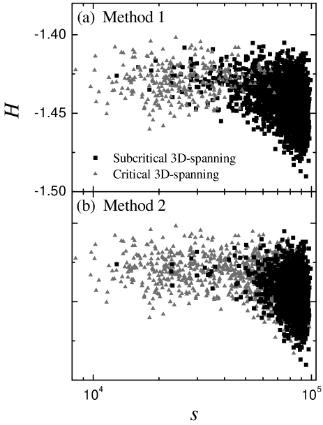
Figure 6: Example of separation of 3D-spanning avalanches into subcritical and critical, using methods 1 and 2 explained in the text.

The two separation methods will be used throughout the rest of the text to separately analyze the data corresponding to subcritical 3D-spanning avalanches and critical 3D-spanning avalanches. In some of the statistical analysis presented below we will consider only the 3D-spanning avalanches which are equally classified by the two methods and discard those which are classified differently from the analysis. Although this procedure reduces the size of the statistical sample, it ensures that we do not introduce any bias due to ill-classification of some of the avalanches.

V Scaling collapses

V.1 Field Averages and standard deviations

Fig. 7 presents the scaling collapses corresponding to the field averages for $\sigma\leq\sigma_{c}$. Data is presented on log-log scales in order to analyze the power-law behavior for $|u|L^{1/\nu}\rightarrow\infty$. Fig. 7(a) shows data corresponding to $\langle H\rangle_{1}$, $\langle H\rangle_{2}$, and $\langle H\rangle_{3c}$, whereas Fig. 7(b) shows data corresponding to $\langle H\rangle_{3-}$. We remark that only the 3D-spanning avalanches equally classified by Methods 1 and 2 have been used for computing the averages corresponding to $\langle H\rangle_{3-}$ and $\langle H\rangle_{3c}$. By fixing $1/\mu=1.5$ and taking $\nu=1.2$ from Ref. Pérez-Reche and Vives (2003) we get the best collapses for $B^{\prime}=0.25\pm 0.10$. We would like to emphasize that the four sets of data scale extremely well with the same values of $\mu$ and $\nu$.

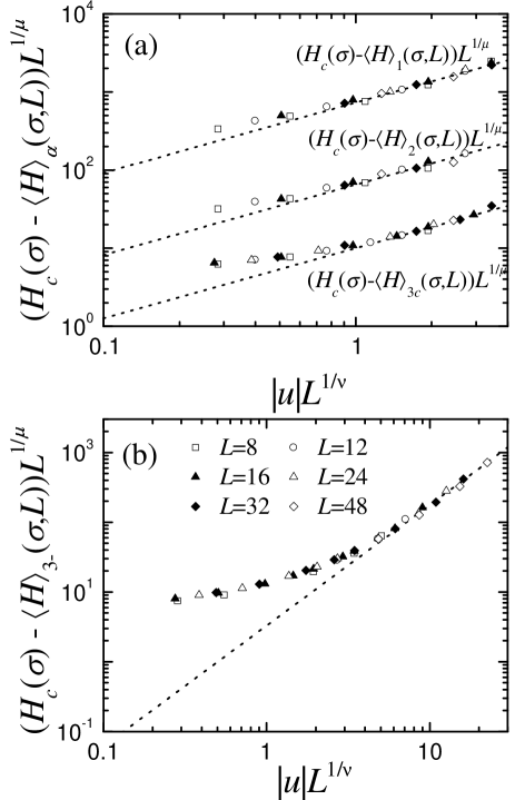
Figure 7: Scaling plots corresponding to the difference between $\langle H\rangle_{\alpha}$ and the effective critical disorder $H_{c}(\sigma)$ for (a) 1D-, 2D-, and critical 3D-spanning avalanches and (b) the subcritical 3D-spanning avalanches. We present only data for $\sigma<\sigma_{c}$. The dotted lines correspond in each case to the asymptotic behavior of $-\hat{h}_{\alpha}$ when $|u|L^{1/\nu}\rightarrow\infty$. The scaling plots corresponding to the 1D- and 2D-spanning avalanches have been displaced one decade upwards for clarity.

The asymptotic behavior of ${\hat{h}}_{3-}$ (dotted line in Fig. 7(b)) for large values of $|u|L^{1/\nu}$ is $3.3\left(|u|L^{1/\nu}\right)^{1.8}$. The exponent $1.8$ equals $\nu/\mu$ within statistical error. This means that, in the thermodynamic limit,

$$\langle H\rangle_{3-}(\sigma)=H_{c}^{\ast}(\sigma)-3.3|u|^{\nu/\mu}.$$ (31)

Fig. 8 shows this behavior, which finishes at the critical point $(\sigma_{c},H_{c})$ because no subcritical 3D-spanning avalanches exist above. The disorder-dependent critical field $H^{\ast}_{c}(\sigma)$ and the critical field $H_{c}$ are indicated by dashed and dotted lines, respectively. We have also plotted the numerical estimates of $\langle H\rangle_{3-}$ for different system sizes in order to show that Eq. (31) is the limiting behavior for $L\rightarrow\infty$.

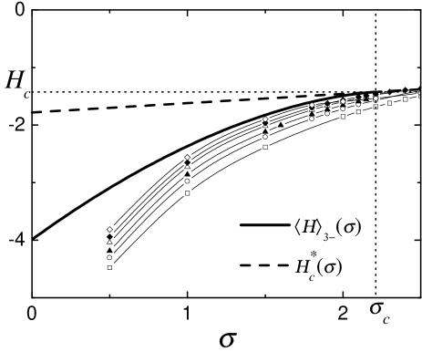
Figure 8: Representation of $\langle H\rangle_{3-}(\sigma)$ (Eq. (31)), $H^{\ast}_{c}(\sigma)$ (Eq. (29)), and $H_{c}$. Symbols correspond to the numerical estimate of $\langle H\rangle_{3-}$ from simulations for different $L$, as indicated by the legend in the previous figure.

The asymptotic behavior of $\hat{h}_{\alpha}$ for the 1D-, 2D- and critical 3D-spanning avalanches is proportional to $\left(|u|L^{1/\nu}\right)^{0.9}$. This implies that in the thermodynamic limit

$$\langle H\rangle_{\alpha}(\sigma)=H^{\ast}_{c}(\sigma)$$ (32)

for the 1D-, 2D- and critical 3D-spanning avalanches.

Similar finite-size scaling analyses can be done for the standard deviations of the marginal distributions $n_{\alpha}/N_{\alpha}$ according to Eq. (30). From the obtained collapses we deduce the following behavior for large values of $|u|L^{1/\nu}$ ($\sigma<\sigma_{c}$): $\hat{\sigma}_{3-}^{H}(uL^{1/\nu})\sim(|u|L^{1/\nu})^{0.6}$ for the subcritical 3D-spanning avalanches and $\hat{\sigma}_{3c}^{H}(uL^{1/\nu})\sim(|u|L^{1/\nu})^{0.2}$ for the 1D-, 2D-, and critical 3D-spanning avalanches. Similar behavior is observed for $\sigma>\sigma_{c}$. These results (see Eq. (30)) indicate that the standard deviation of the marginal distribution $n_{\alpha}/N_{\alpha}$ corresponding to any type of spanning avalanche vanishes in the thermodynamic limit for any value of $\sigma$.

V.2 Number density

The number density corresponding to the 1D-spanning avalanches at the critical amount of disorder $n_{1}(H;\sigma_{c},L)$ is shown in Fig. 9(a) as a function of the applied field for different system sizes. The number density shows a peak that increases and shifts for increasing $L$. Similar behavior is observed for $n_{2}(H;\sigma_{c},L)$ (Fig. 10(a)). A FSS analysis is performed using the scaling assumption for the number densities (Eq. (17)). The results of such an analysis are presented in Figs. 9(b) and 10(b) for $n_{1}(H;\sigma_{c},L)$ and $n_{2}(H;\sigma_{c},L)$, respectively. To obtain these collapses we have used $\theta=0.1$ and $1/\mu=1.5$ as in the preceding sections. The scaling functions in Figs. 9(b) and 10(b) are well approximated by Gaussian functions (indicated by continuous lines). When $vL^{1/\mu}\rightarrow\pm\infty$ both scaling functions go exponentially to zero. This behavior indicates that, in the thermodynamic limit for $\sigma=\sigma_{c}$, 1D- and 2D-spanning avalanches only exist at $H=H_{c}$.

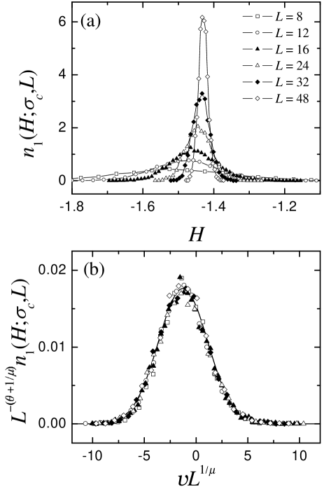
Figure 9: (a) Number density of spanning avalanches in one dimension at the critical amount of disorder. (b) Scaling plot corresponding to the data in (a) according to Eq. (17) with $\theta=0.1$. The continuous line in (b) shows a Gaussian fit.

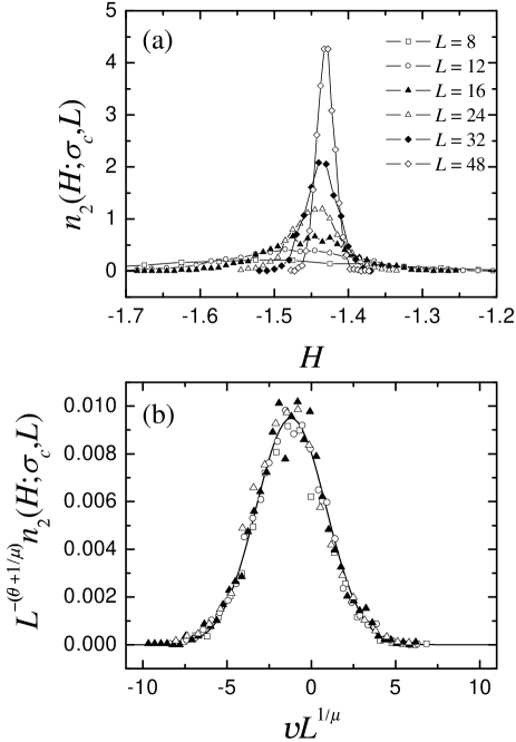
Figure 10: (a) Number density of spanning avalanches in two dimensions at the critical amount of disorder. (b) Scaling plot corresponding to the data in (a) according to Eq. (17) with $\theta=0.1$. The continuous line in (b) shows a Gaussian fit.

Fig. 11 shows several cuts corresponding to the scaling surface $\hat{n}_{1}(uL^{1/\nu},vL^{1/\mu})$. From the collapses we obtain $B^{\prime}=0.25\pm 0.10$ in total agreement with previous estimates. From a qualitative point of view, the collapses indicate that the scaling surface shows a crest with amplitude depending on $uL^{1/\nu}$. More quantitatively, the scaling collapses for each cut can be well approximated by Gaussian functions, whose amplitude, peak position, and width depend on $uL^{1/\nu}$. Furthermore, the dependence on $uL^{1/\nu}$ of the fitted amplitudes also adjusts very well to a Gaussian function that follows the profile of the crest (continuous line on the back plane in Fig. 11). The dashed line on the bottom plane indicates the position of the crest $\langle vL^{1/\mu}\rangle_{1}(uL^{1/\nu})=\hat{h}_{1}(uL^{1/\nu})/H_{c}$, which has already been shown in Fig. 7(a).

All these considerations imply that, for any value of $H$, the scaling function $\hat{n}_{1}$ decays exponentially when $uL^{1/\nu}\rightarrow\pm\infty$. This indicates that, in the thermodynamic limit, irrespective of the value of $H$, $n_{1}$ is zero for $\sigma\neq\sigma_{c}$. In contrast, when $\sigma=\sigma_{c}$, $n_{1}$ diverges at $H=H_{c}$ and is zero for other values of the field. This scenario for $n_{1}$ is also applicable to $n_{2}$.

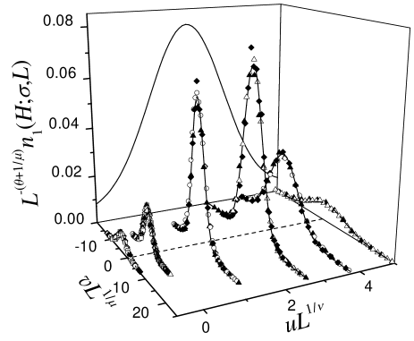
Figure 11: Collapses corresponding to $\hat{n}_{1}(uL^{1/\nu},vL^{1/\mu})$. The cuts of the scaling surface are taken at $uL^{1/\nu}=-0.58,0,1.22,2.7,3.8$ and $5.0$. Symbols correspond to the sizes indicated in the legend of the previous figure. The dashed line on the horizontal plane indicates the tendency of the crest of the scaling surface. The projection of the crest (Gaussian fit) is depicted with a continuous line on the plane $uL^{1/\nu}$-$\hat{n}_{1}$.

To obtain $n_{3c}$ and $n_{3-}$ we have used Method 2 of separation described in Sec. IV.4. The results for $\sigma=\sigma_{c}$ are presented in Figs. 12 and 13 for $n_{3c}(H;\sigma_{c},L)$ and $n_{3-}(H;\sigma_{c},L)$, respectively. We have also tried to separate the two kinds of avalanches by Method 1, but the collapses are not as good as those obtained with Method 2. This result indicates that in the set of avalanches non-equally classified by the two methods, there are more critical 3D-spanning avalanches than subcritical 3D-spanning avalanches.

As in the case of $n_{1}$ and $n_{2}$ at $\sigma=\sigma_{c}$, the behavior of the scaling functions in Figs. 12(b) and 13(b) indicate that both $n_{3c}$ and $n_{3-}$ diverge at $H=H_{c}$ and are zero for fields different to $H_{c}$.

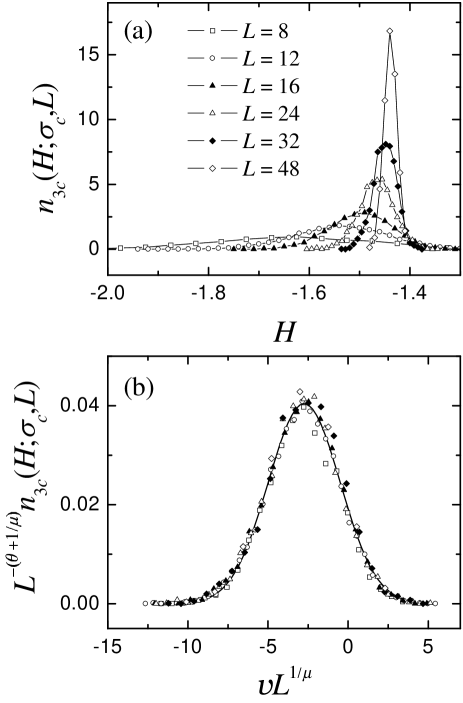
Figure 12: (a) Number density of critical 3D-spanning avalanches at the critical amount of disorder obtained using Method 2. (b) Scaling plot corresponding to the data in (a) according to Eq. (17) with $\theta=0.1$.

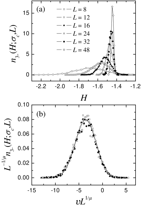
Figure 13: (a) Number density of subcritical 3D-spanning avalanches at the critical amount of disorder obtained using Method 2. (b) Scaling plot corresponding to the data in (a) according to Eq. (17) with $\theta=0$.

The detailed study of the bivariate collapses corresponding to $n_{3c}(H;\sigma,L)$ and $n_{3-}(H;\sigma,L)$ for $\sigma\neq\sigma_{c}$ is difficult and tedious. In particular, for $\sigma>\sigma_{c}$ we do not expect the separation methods to work and for $\sigma<\sigma_{c}$, the analysis would require a lot of statistics.

VI Direct determination of the fractal dimensions

In the thermodynamic limit we assume the standard fractal behavior, i.e. that the average mass belonging to a certain avalanche type inside a box of linear size $\ell$ is given by:

$$M_{\alpha}(\ell;\sigma)=M_{\alpha}^{\ast}(\sigma)\ell^{d_{\alpha}}$$ (33)

in the limit $\ell\ll\xi$, where $\xi$ is the correlation length. The prefactor $M_{\alpha}^{\ast}(\sigma)$ is related to the concept of lacunarity B.B.Mandelbrot (1983). In general there can be fractals sharing the same fractal dimension, but with different lacunarities. The fractal dimension is related to the rate of change of the mass when the size of the box is changed. In contrast, the lacunarity is related to the size of the gaps of the fractal and is independent of the fractal dimension. In this way, the larger the typical size of the gaps, the higher the lacunarity. For many fractals, B.B.Mandelbrot (1983); C.Allain and M.Cloitre (1991) as lacunarity increases, the prefactor $M_{\alpha}^{\ast}$, decreases since the mass inside a box of linear size $\ell$ decreases.

For finite systems it is necessary to translate the law (33) into a finite-size scaling hypothesis. As usually done, we propose:

$$M_{\alpha}(\ell;\sigma,L)=L^{d_{\alpha}}\hat{M}_{\alpha}(uL^{1/\nu},\ell/L)\;;\hskip 19.91684pt\xi\lesssim L,$$ (34)

where the condition $\xi\lesssim L$ stands for the fact that scaling only holds in the critical zone. Eq. (34) allows the data corresponding to the masses $M_{\alpha}$ to be collapsed and, in this way, to obtain the fractal dimensions $d_{\alpha}$. We can predict the shape of $\tilde{M}_{\alpha}$ in two limiting cases: on the one hand, the scaling function $\hat{M}_{\alpha}(uL^{1/\nu},\ell/L)$ should behave as:

$$\hat{M}_{\alpha}(uL^{1/\nu},\ell/L)=M_{\alpha}^{\ast}(uL^{1/\nu})\left(\frac{\ell}{L}\right)^{d_{\alpha}},$$ (35)

in the limit $\ell/L\ll\xi/L\lesssim 1$ to recover the expression (33) from (34). On the other hand, in the limit $\ell/L\gg\xi/L$, the scaling function corresponding to the subcritical 3D-spanning avalanche should behave as

$$\hat{M}_{3-}(uL^{1/\nu},\ell/L)\sim\left(|u|L^{1/\nu}\right)^{\beta_{3-}}\left(\frac{\ell}{L}\right)^{3},$$ (36)

if this avalanche fills a finite fraction $|u|^{\beta_{3-}}$ of the system for $\sigma<\sigma_{c}$ in the thermodynamic limit Vives and Pérez-Reche (2004) and we expect

$$M_{3-}(\ell;\sigma)\sim|u|^{\beta_{3-}}\ell^{3}.$$ (37)

Such behavior can be obtained from Eqs. (36) and (34) using the hyperscaling relation $\beta_{3-}=\nu(3-d_{3-})$.

Fig. 14 shows the scaled mass for all kinds of spanning avalanches from simulations performed at $\sigma=\sigma_{c}$. We have only considered the mass of those 3D-spanning avalanches that are equally classified by the two proposed methods. The fractal dimension rendering the best collapse is $d_{f}=2.78\pm 0.05$ for the 1D-, 2D-, and critical 3D-spanning avalanches and $d_{3-}=2.98\pm 0.02$ for the subcritical 3D-spanning avalanches. Both values are in total agreement with those obtained independently in Pérez-Reche and Vives (2003). Moreover, the slope of each collapse in the limit $\ell\ll L$ (left-hand side of the collapses) coincides with the fractal dimension used to obtain the collapses, so that the behavior (35) is confirmed. The prefactors are $M_{1}^{\ast}(\sigma_{c})=0.95\pm 0.07$, $M_{2}^{\ast}(\sigma_{c})=0.93\pm 0.07$, $M_{3c}^{\ast}(\sigma_{c})=0.90\pm 0.07$, and $M_{3-}^{\ast}(\sigma_{c})=0.65\pm 0.07$. The low value of the prefactor corresponding to the subcritical 3D-spanning avalanches indicates that the gaps of these avalanches are large. As a consequence, the space filled locally by these avalanches is not as high as one would a priori think given the proximity of $d_{3-}$ to 3.

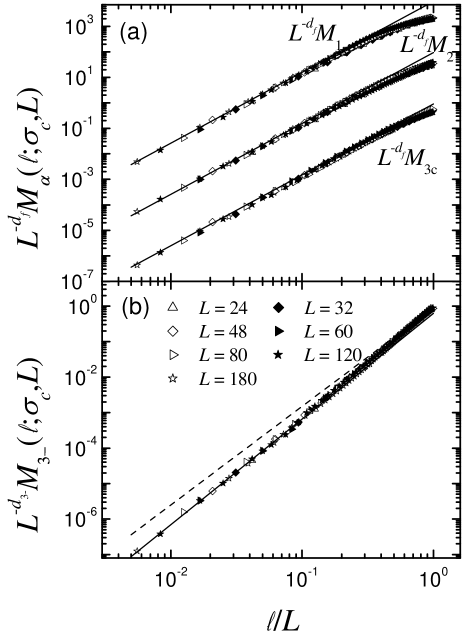
Figure 14: (a) Scaling collapses corresponding to the mass of the 1D-, 2D-, and critical 3D-spanning avalanches at $\sigma=\sigma_{c}$. The collapses corresponding to $M_{1}$ and $M_{2}$ have been displaced two decades upwards for clarity. (b) Scaling of $M_{3-}$ also at $\sigma=\sigma_{c}$. In all cases the asymptotic behavior for small values of $\ell/L$ has been indicated by continuous lines. The dashed line in (b) corresponds to the assimptotic behavior of $\hat{M}_{3c}$ to compare it with $\hat{M}_{3-}$.

To study the behavior of $M_{3-}$ for $\sigma<\sigma_{c}$ it is convenient to multiply the scaling function $\tilde{M}_{3-}$ by the factor $(\ell/L)^{-3}$. From Eqs. (35) and (36), it should behave as:

$$\left(\frac{\ell}{L}\right)^{-3}\tilde{M}_{3-}=\begin{cases}M^{\ast}_{3-}(uL^{1/\nu})\left(\frac{\ell}{L}\right)^{d_{3-}-3}&,\frac{\ell}{L}\ll\frac{\xi}{L}\\ \sim\left(|u|L^{1/\nu}\right)^{\beta_{3-}}&,\frac{\ell}{L}\gg\frac{\xi}{L}\end{cases}$$ (38)

in such a way that, for a given value of $uL^{1/\nu}<0$, the function $(\ell/L)^{-3}\tilde{M}_{3-}$ approaches a constant value for large values of $\ell/L$ if the correlation length is finite. Fig. 15 shows the scaling collapses of $(\ell/L)^{-3}\tilde{M}_{3-}$ for three cuts of the scaling surface taken at $uL^{1/\nu}=-3.73,-7.41$ and $-13.18$. Note that such cuts are limited from below at $\ell/L=1/80$. In spite of this limitation, the results clearly indicate that (i) for small values of $\ell/L$, the behavior of $(\ell/L)^{-3}\tilde{M}_{3-}$ is power law with an exponent approaching $d_{3-}-3\simeq 0.02$ (indicated by the dotted line) and (ii) for large values of $\ell/L$ the function $(\ell/L)^{-3}\tilde{M}_{3-}$ tends to a constant value. (This latter tendency can only be observed for negative enough values of $uL^{1/\nu}$) and confirms the hypothesis in Eq. (38). Therefore, one can deduce that $\xi/L$ is finite for $\sigma<\sigma_{c}$ and it decreases when $uL^{1/\nu}$ becomes more negative. In addition, the results confirm the compact character of the subcritical 3D-spanning avalanche, as proposed in Ref. Vives and Pérez-Reche (2004) by a different method.

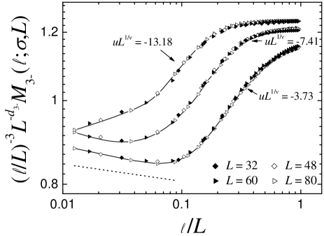
Figure 15: Collapses corresponding to $(\ell/L)^{-3}\tilde{M}_{3-}(uL^{1/\nu},\ell/L)$ for $uL^{1/\nu}=-3.73,-7.41$ and $-13.18$. The dashed line indicates the slope $d_{3-}-3=0.02$. Continuous lines are a guide to the eye.

VII Discussion

The results presented so far together with the results obtained in Ref. Pérez-Reche and Vives (2003) provide a clear scenario for the phase diagram of the $T=0$ 3D-GRFIM with metastable dynamics in the thermodynamic limit.

We have deduced that the subcritical 3D-spanning avalanche occurring on the transition line given by Eq. (31) is compact and is thus responsible for the macroscopic jump of the magnetization Pérez-Reche and Vives (2003). Therefore we are facing a standard first-order phase transition scenario with no divergence of the correlation length for $\sigma<\sigma_{c}$. At the critical point, this subcritical 3D-spanning avalanche becomes fractal at all length scales, and does not fill any finite fraction of the system. The end point $(\sigma_{c},H_{c})$ is a standard critical point.

Fig. 16(a) shows the obtained phase diagram. The dashed line represents the first-order transition line given by Eq. (31) and the large dot the critical point. Note that this transition line is only approximate because it has been deduced from scaling arguments close to the critical point. Nevertheless it is remarkable that Eq. (31) for $\sigma=0$ renders $\langle H\rangle_{3-}(0)=-3.999$ which is unbelievably close to the value $-4$ which can be computed by a (not so) trivial analysis of the coercive field of the hysteresis loop of the Gaussian 3d-RFIM with metastable dynamics corresponding to $\sigma\rightarrow 0^{+}$.

In Fig. 16(b) we also show for comparison the phase diagram of the 3D-GRFIM model in equilibrium at $T=0$ (ground-state) Middleton and D.S.Fisher (2002). In addition, in Figs. 16 (c) and (d) we show the mean field (MF) solutions corresponding to both the metastable Sethna et al. (1993) and equilibrium T.Schneider and E.Pytte (1977) cases.

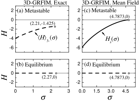
Figure 16: Phase diagram corresponding to the exact 3D-GRFIM with metastable dynamics (a) and in equilibrium (b). The phase diagrams corresponding to the mean field approximation of the 3D-GRFIM with metastable dynamics (c) and in equilibrium (d) are also shown. The thick continuous line in (c) indicates the spinodal transition in the metastable solution and the dashed lines in (a), (b), and (d) indicate the first-order transitions. In all cases we have indicated the coordinates of the critical point.

The MF scenario indicates that the equilibrium and metastable critical points occur for the same value of $\sigma_{c}=z\sqrt{2/\pi}$ (Table 4), where $z$ is the coordination number. In particular, $z=6$ renders $\sigma_{c}=4.7873$ for the 3D-GRFIM. Below $\sigma_{c}$, nevertheless, the transition in equilibrium is a standard first-order transition (at $H=0$), whereas it is a spinodal line $H_{s}(\sigma)$ in the metastable case. From the equations in Refs. Sethna et al., 1993 and Dahmen and J.P.Sethna, 1996 it can be found that the metastability limit is:

$$H_{s}(\sigma)=\sigma\sqrt{2\ln\frac{\sigma_{c}}{\sigma}}-z\Phi_{err}\left(\sqrt{\ln\frac{\sigma_{c}}{\sigma}}\right),$$ (39)

when the external field is decreased. $\Phi_{err}$ is the error function. The continuous line in Fig. 16(c) corresponds to $H_{s}(\sigma)$ for $z=6$. The spinodal transition is characterized by a divergence of the fluctuations and the correlation length on the line $H_{s}(\sigma)$ where the discontinuity of the order parameter $\Delta m$ occurs.

In the present work we have shown that when comparing the exact solutions (non MF) of both the equilibrium model and the metastable model, the character of the transition line does not change. In both cases the transitions are standard first-order transitions with order parameter discontinuities and finite correlation length. This result agrees with the prediction Dahmen and J.P.Sethna (1996) that the transition is abrupt for $d<8$ as deduced from an $\epsilon$ expansion analysis around $d=8$.

As indicated in Fig. 16 and Table 4, $\sigma_{c}^{eq}=2.270\pm 0.004$ in equilibrium and $\sigma_{c}^{met}=2.21\pm 0.02$ in the metastable case. Regarding the value of the critical field, it is $|H_{c}|=1.425$ in the exact metastable model and zero in the exact equilibrium model. Thus, when the exact 3d-GRFIM is studied, the critical point in equilibrium does not coincide with that corresponding to metastable dynamics. Nevertheless, the critical exponents are the same within statistical errors. The values are indicated in Table 4. In fact, Dahmen et al. Dahmen and J.P.Sethna (1996) have already pointed out this similitude between the critical exponents for both models. These authors argue that agreement between the two sets of exponents is rather unexpected since the two models are very different.

Magnitude	3D-GRFIM. Mean field		3D-GRFIM
	Equilibrium	Metastable	Equilibrium	Metastable
	(Ref. T.Schneider and E.Pytte (1977))	(Ref. O.Perković et al. (1996))	(Ref. Middleton and D.S.Fisher (2002))	(This work)
$\sigma_{c}$	$z\sqrt{2/\pi}$	$z\sqrt{2/\pi}$	$2.270\pm 0.004$	$2.21\pm 0.02$
$|H_{c}|$	0	0	0	$1.425\pm 0.010$
$\nu$	$1/2$	$1/2$	$1.37\pm 0.09$	$1.2\pm 0.1$
$1/\mu$	3	3	$1.498\pm 0.034$	$1.5\pm 0.1$
$\beta$	$1/2$	$1/2$	$0.017\pm 0.005$	$0.024\pm 0.012$

Table 4: Coordinates of the critical point in the $\sigma-H$ plane and critical exponents for the 3D-GRFIM in equilibrium and with metastable dynamics corresponding to the MF approximation and the exact models.

Nevertheless, we can provide an argument based on renormalization group theory that indicates that the critical points in the two models (3D-RFIM in equilibrium and the 3D-RFIM with metastable dynamics) correspond to the same fixed point in a more general parameter space. Within the framework of RG theory the critical surface (or critical line) is defined as the set of all points in the parameter space that flow to a certain critical fixed point when the renormalization group transformation is applied. The variation of the tunable parameters of a model describes a “physical” trajectory in the parameter space. According to these definitions, the critical point corresponds to the point where the “physical” trajectory intersects the critical surface. The two models discussed here can be considered as particular cases of a more general model with the same 3D-GRFIM Hamiltonian and the following $T=0$ adiabatic dynamics: when $B$ is varied, blocks of neighboring spins of size $n\leq n_{max}$ flip when such a flip represents an energy decrease. The metastable dynamics introduced by Sethna corresponds to $n_{max}=1$ (only single spin flips are considered) and the equilibrium model at $T=0$ (exact ground-state) corresponds to $n_{max}=\infty$. The parameter $n_{max}$ is a new parameter that must be considered in the RG equations. Since a critical point is found both with $n_{max}=1$ and $n_{max}=\infty$, it is natural to assume that this is an irrelevant parameter. Thus, we propose the scenario presented in Fig. 17. Changing $n_{max}$ alters the position of the critical point, but not the critical exponents which correspond to the same critical fixed point. Numerical simulations of the 3D-GRFIM with $n_{max}>1$ dynamics will help in clarifying this picture. At present we guess that the RG flow follows the arrows schematically indicated in Fig. 17. Both the equilibrium critical point (ECP) and the metastable critical point (MCP) lie on the same critical surface (CS). In general a first-order phase transition occurs at the points in the parameter space that go towards a discontinuity fixed point when the RG transformation is applied. B.Nienhuis and M.Nauenberg (1975) We assume the existence of two discontinuity fixed points: the equilibrium discontinuity fixed point (EDFP) and the metastable discontinuity fixed point (MDFP). The EDFP controls the first-order phase transition in the equilibrium case ($n_{max}^{-1}=0$ and $\sigma<\sigma_{c}^{eq}$) and the MDFP controls the first-order phase transition when $n_{max}^{-1}>0$. All the points that flow towards any of the discontinuity fixed points define the discontinuity surface (DS) where the first-order phase transition occurs.

Figure 17: Schematic phase diagram of the proposed model in the space $(H,n_{max}^{-1},\sigma)$ in the adiabatic limit and $T=0$. Arrows indicate the RG flow. The meaning of the different acronyms is explained in the text. The grey lines correspond to projections on the vertical planes.

Another interesting question to be discussed is the determination of the correlation length $\xi$ in the 3D-GRFIM with metastable dynamics. Avalanches can be understood as the zero temperature fluctuations in the driven system. Is their average linear size related to $\xi$?. The first thing to note is that we have found that avalanches display two different fractal dimensions (and thus different associated $\beta$ exponents). The $\nu$ and $\mu$ exponents, nevertheless, are the same for all the scaling collapses. For instance, this is illustrated by Fig. 7 in this work and by Figs. 8, 9, and 10 in Ref. Pérez-Reche and Vives (2003). Thus the behavior of the correlation length is unique:

$$\xi=u^{-\nu}\hat{\Xi}(u^{\nu}v^{-\mu}),$$ (40)

with $\hat{\Xi}(x)\sim x+{\cal O}(x^{2})$. The fluctuations then can “choose” between two different mechanisms for propagation either with fractal dimension $d_{f}=2.78$ or with fractal dimension $d_{3-}=2.98$. The second point to be considered is that $\xi$ cannot be related to the size of the subcritical 3D-spanning avalanche since we have found that $\xi$ is finite below $\sigma_{c}$. Keeping these two observations in mind we propose that the correlation length is related to the average radius of the largest non-spanning avalanche. Below $\sigma=\sigma_{c}$ the existence of a compact subcritical 3D-spanning avalanche does not allow for the non-spanning avalanches to overcome a certain finite length and thus $\xi$ is finite. Only at the critical point does the subcritical 3D-spanning avalanche become fractal and allows for other spanning avalanches to exist and $\xi$ becomes infinite. This behavior is much similar to what has been recently found in percolation. Aizenman (1997); Stauffer (1997) We conjecture that some of the theorems that have been rigorously proven concerning the uniqueness of the infinite percolating cluster should be applicable to our case concerning the compact subcritical 3D-spanning avalanche. The present results should be considered as an interesting stimulus to proceed with the analysis of percolation theory. For instance, we propose checking whether the fractal dimension of the spanning clusters is the same as that of the infinite cluster at distances lower than the correlation length at the percolation threshold.

VIII Summary and conclusions

The results presented in this paper are mainly related to two topics in the 3D-GRFIM: firstly, the field dependence of the spanning avalanches, and secondly, the geometrical properties of the avalanches. We have extended the FSS hypothesis proposed in Pérez-Reche and Vives (2003) to properly take into account the field dependence of the number densities $n_{\alpha}(H,\sigma,L)$ and of the bivariate distributions ${\cal D}_{\alpha}(s,H;\sigma,L)$. When carrying out such an extension, it is necessary to introduce a new scaling variable $v$ and a new exponent $\mu$ related to the divergence of the correlation length when $H$ approaches $H_{c}$ ($\xi\sim(H-H_{c})^{-\mu}$). We have also introduced a scaling hypothesis for the field $\langle H\rangle_{\alpha}(\sigma,L)$ at which the different avalanches concentrate and their standard deviation $\sigma_{\alpha}^{H}(\sigma,L)$. From the scaling collapses corresponding to the 1D- and 2D-spanning avalanches we have found $1/\mu=1.5$. The study of the 3D-spanning avalanches is more intricate as already shown in Pérez-Reche and Vives (2003), where we propose the existence of two different kinds of 3D-spanning avalanches. In this paper we have proposed two approximate separation methods for classifying these avalanches as subcritical or critical. Using these methods we have found that $1/\mu=1.5$ for both cases. Scaling enables the following behavior to be scketched in the thermodynamic limit: The 1D-, 2D-, and critical 3D-spanning avalanches only exist at the critical point $(\sigma_{c},H_{c})=(2.21,-1.425)$, where their number densities are infinite. In contrast, one subcritical 3D-spanning avalanche exists below $\sigma_{c}$ and it occurs on the line $\langle H\rangle_{3-}(\sigma)$ (Eq. (31)).

From the average mass $M_{\alpha}(\ell;\sigma)$ we have obtained the fractal dimensions corresponding to each of the types of spanning avalanches. This has allowed us to confirm independently the results in Pérez-Reche and Vives (2003): $d_{f}=2.78\pm 0.05$ for the 1D-, 2D-, and subcritical 3D-spanning avalanches and $d_{3-}=2.98\pm 0.02$. Furthermore, the behavior for $\sigma<\sigma_{c}$ of the mass corresponding to the subcritical 3D-spanning avalanches indicates that the correlation length $\xi$ is finite below $\sigma_{c}$. As a consequence, we conclude that the line $\langle H\rangle_{3-}(\sigma)$, where the discontinuity in the order parameter occurs, corresponds to a standard first-order phase transition line and $\xi$ only diverges at the critical point.

References

- J.P.Sethna et al. (2001) J.P.Sethna, K.A.Dahmen, and C.R.Myers, Nature 410, 242 (2001).
- Babcock and Westervelt (1990) K. Babcock and R. Westervelt, Phys. Rev. Lett. 64, 2168 (1990).
- P.J.Cote and L.V.Meisel (1991) P.J.Cote and L.V.Meisel, Phys. Rev. Lett. 67, 1334 (1991).
- Puppin (2000) E. Puppin, Phys. Rev. Lett. 84, 5415 (2000).
- M.P.Lilly et al. (1993) M.P.Lilly, P.T.Finley, and R.B.Hallock, Phys. Rev. Lett. 71, 4186 (1993).
- E.Kierlik et al. (2001) E.Kierlik, P.A.Monson, M.L.Rosinberg, L.Sarkisov, and G.Tarjus, Phys. Rev. Lett. 87, 055701 (2001).
- Vives et al. (1994) E. Vives, J. Ortín, L. Mañosa, I. Ràfols, R. Pérez-Magrané, and A. Planes, Phys. Rev. Lett. 72, 1694 (1994).
- (8) F. Casanova, A. Labarta, X. Batlle, E. V. J. Marcos, Ll.Mañosa, and A. Planes, to be published.
- F.J.Pérez-Reche et al. (2001) F.J.Pérez-Reche, E.Vives, L. Mañosa, and A.Planes, Phys. Rev. Lett. 87, 195701 (2001).
- Vives and Planes (1994) E. Vives and A. Planes, Phys. Rev. B 50, 3839 (1994).
- Carrillo et al. (1998) L. Carrillo, Ll.Mañosa, J. Ortín, A. Planes, and E.Vives, Phys. Rev. Lett. 81, 1889 (1998).
- Sethna et al. (1993) J. P. Sethna, K. Dahmen, S. Kartha, J. A. Krumhansl, B. W. Roberts, and J. D. Shore, Phys. Rev. Lett. 70, 3347 (1993).
- Dahmen and J.P.Sethna (1993) K. A. Dahmen and J.P.Sethna, Phys. Rev. Lett. 71, 3222 (1993).
- Perković et al. (1995) O. Perković, K. A. Dahmen, and J.P.Sethna, Phys. Rev. Lett 75, 4528 (1995).
- Dahmen and J.P.Sethna (1996) K. A. Dahmen and J.P.Sethna, Phys. Rev. B 53, 14872 (1996).
- Tadić (1996) B. Tadić, Phys. Rev. Lett. 77, 3843 (1996).
- Perković et al. (1999) O. Perković, K. A. Dahmen, and J.P.Sethna, Phys. Rev. B 59, 6106 (1999).
- Kuntz et al. (1999) M. C. Kuntz, O. Perković, K. A. Dahmen, B. Roberts, and J.P.Sethna, Computing in Science & Engineering July/August, 73 (1999).
- J.H.Carpenter and K.A.Dahmen (2002) J.H.Carpenter and K.A.Dahmen, cond-mat/0205021 (2002).