First pacs description Second pacs description

Nonstationary dephasing of two level systems

Abstract

We investigate the influence of nonstationary $1/f^{\mu}$ noise, produced by interacting defects, on a quantum two-level system. Adopting a simple phenomenological model for this noise we describe exactly the corresponding dephasing in various regimes. The nonstationarity and pronounced non-Gaussian features of this noise induce new anomalous dephasing scenarii. Beyond a history-dependent critical coupling strength the dephasing time exhibits a strong dependence on the age of the noise and the decay of coherence is not exponential.

The question of the phase coherence of a quantum two level system (TLS) in a noisy environment has motivated numerous recent works. In particular it is of crucial interest in the context of quantum computing with solid state quantum bits[1]. In this case it is now believed that dephasing of the TLS by a low-frequency ($1/f$) noise is a limiting mechanism which certainly deserves further studies. The microscopic origin of these low-frequency fluctuations depends on the considered system and is mostly not understood[2]. Hence, in previous works on this problem the $1/f$ environment was modeled phenomenologically either by a set of harmonic modes (e.g. spin-Boson model)[3] or by an ensemble of independent bistable fluctuators (Dutta-Horn model)[4, 5]. The first model assumes a Gaussian distribution for the fluctuations and stationarity of the noise. As this low frequency noise appears to be an essentially out of equilibrium phenomenon, this last hypothesis is questionable[6]. The Dutta-Horn model does not suffer from this restriction[5], but assumes the presence of a broad distribution of relaxation times for the independent fluctuators, or equivalently a flat distribution for their random energy barriers. However, both the nature of these fluctuators and the origin of these long relaxation times are beyond the current experimental knowledge. We consider the interactions between the fluctuators as a possible source for these slow dynamics. In this letter, we explore the consequences of this interaction on the nonstationarity of the dephasing by considering a simple phenomenological model for a strongly coupled cluster of fluctuators.

Let us thus consider a dissipative quantum two-level system (qubit) described by the Hamiltonian :

$${\cal H}=\epsilon\>\sigma^{z}+\Delta\>\sigma^{x}-\frac{1}{2}X\>\sigma^{z}\;,$$ (1)

where $\epsilon$ and $\Delta$ are control parameters which we assume to be time-independent and $X$ describes the fluctuating extra bias (noise) induced by the environment. In this letter, we focus on the case $\Delta=0$. However, extensions to the case $\Delta\neq 0$ and a low frequency noise $X$ may be treated along the lines of ref. [3]. Within a Dutta-Horn model[5, 6], the noise $X$ consists in the sum of contributions from independent fluctuators, modeled as random two-level systems coupled to an equilibrium bath (e.g. the phonons). This bosonic bath induces an elastic or electromagnetic coupling between the qubit and each fluctuator but also mutual couplings of same origin between the fluctuators which are usually neglected. This interaction depends on the nature of the coupling to the bath : both elastic strain (phonons) and dipolar electric coupling correspond to a long-range dipolar interaction[7, 8] The motivation to consider such couplings between the fluctuators comes in part from the analogous physics of TLS in amorphous solids: the relevance of these TLS couplings was stressed by Yu and Leggett [9], and found recent experimental evidence in the dielectric response of amorphous films[10]. These interactions are a possible source of broad distribution of relaxation times of the bath : in particular, using the language of pseudospins for the fluctuators, a strong ferromagnetic coupling between an ensemble of $N$ spins forces these spins to tunnel simultaneously, therefore reducing exponentially with the size $N$ the tunneling amplitude of the cluster. Such a nonlinear relation between the size of a cluster and the corresponding relaxation time would naturally lead to a broad distribution for these times. Moreover, for randomly located fluctuators elastically coupled, we expect the interactions to be random and frustrating [7]. It is then natural to consider the noise produced by a mesoscopic ensemble of $N$ interacting fluctuators[11]. We expect these interactions and the associated frustration to bring very slow relaxational dynamics for the cluster. However this problem is a formidable task, still unsolved in the case of classical spin glasses. We therefore adopt a phenomenological approach and focus on the expected general consequences of its physics.

As in the case of independent fluctuators [6, 5] we will focus on a classical description of the noise $X(t)$, considering an incoherent environment and neglecting back-action effects of the qubit. A common picture to describe the evolution of a glassy system is a random walk in phase space with broadly distributed time intervals $\tau$ between the ’flips of the environment’. Hence, by analogy with the phase space trap models of classical glassy systems[13], we consider a general random intermittent noise, with randomly distributed heights $x_{i}$ and durations $\tau_{i}^{\uparrow}$ of the plateaus, and waiting times $\tau_{i}$ between them (see Fig.1). For simplicity, we will focus on the case where the $\tau_{i}^{\uparrow}$ are much shorter than the $\tau_{i}$, and given by their average $\tau^{\uparrow}_{0}$. On time scales $\tau\gg\tau_{0}^{\uparrow}$, the plateau is seen as a spike shifting the phase by $x_{i}\tau_{0}^{\uparrow}$. Moreover, to focus on dephasing and eliminate the drift of the accumulated phase of the qubit, the distribution $\mathcal{P}(x)$ is assumed to have zero mean and a finite width $g^{2}=\left<x^{2}\right>(\tau^{\uparrow}_{0})^{2}$: It will be taken as Gaussian without loss of generality. Finally, we consider an algebraic distribution of waiting times $\tau_{i}$ characterized by an exponent $\mu$:

$$P(\tau)=\frac{\mu}{\tau_{0}}\left(\frac{\tau_{0}}{\tau_{0}+\tau}\right)^{1+\mu}\quad,\quad\mathcal{P}(x)=\frac{\tau_{0}^{\uparrow}}{g\sqrt{2\pi}}~{}\exp\left(-\frac{(x\tau^{\uparrow}_{0})^{2}}{2g^{2}}\right)$$ (2)

where $\tau_{0}$ is a microscopic time. The slow algebraic decay of $P(\tau)$ thereby implies divergences of all moments $\overline{\tau^{n}}=\int_{0}^{\infty}d\tau P(\tau)\tau^{n}$ with $n\geq\mu$. It turns out that three different classes of $\mu$ have to be distinguished: (i) If both $\overline{\tau}$ and $\overline{\tau^{2}}$ are finite $(\mu>2)$, the dephasing induced by the noise in our model and within the usual model of Poissonian telegraph noise[6, 5] are identical. Thus, we will call it the Poissonian class. However, in the case of slow dynamics, i.e. for $\mu<2$, the dephasing scenario differs considerably from the Poissonian class. (ii) For $1<\mu<2$, when $\overline{\tau}$ is still finite, but already the second moment $\overline{\tau^{2}}$ diverges, the waiting times $\tau_{i}$ start to fluctuate strongly around their average $\overline{\tau}$ and important corrections with respect to dephasing due to Poissonian class arise. (iii) For $0<\mu<1$, the divergence of the first moment $\overline{\tau}$ makes it even impossible to define a characteristic time between two consecutive spikes. In this case the two-point noise correlation function decays as

$$\overline{X(t+t^{\prime})X(t)}-\overline{X(t)}~{}\overline{X(t+t^{\prime})}\simeq\overline{X(t)}^{2}\left(t/t^{\prime}\right)^{1-\mu}\;,$$ (3)

where the overline denotes an average over realizations of $X(t)$. Eq.(3) implies that the power spectrum exhibits a $1/f^{\mu}$ divergence at low frequencies. Note that the explicit dependence of the correlator (3) on $t$ implies a nonstationarity of the noise and consequently a time dependence of the amplitude of the noise [12]. In our model, a single source of noise with $\mu=1$ can lead to a $1/f$ power spectrum whereas infinitely many independent fluctuators are necessary in the Dutta-Horn approach [5]. Within this latter approach, nonstationary of the noise comes from the choice of initial conditions for the slow fluctuators. In our model, nonstationarity finds its origin in the very slow dynamics underlying the noise, not in a specific choice of an initial condition.

Figure 1: Representation of a noise configuration $X(t)$

The nonstationarity of the noise leads us to pay special attention to the dependence of dephasing on the age of the noise (denoted by $t_{p}$ below), i.e. a history dependence. To be definite we consider situations where the noise has been initialized at time $t^{\prime}=0$. The coupling to the qubit is turned on after a time $t_{\mathrm{p}}$, the preparation time of the qubit. Consequently, the two qubit states $|\pm\rangle$ accumulate a random relative phase between time $t_{\mathrm{p}}$ and $t_{\mathrm{p}}+t$: $\Phi(t_{\mathrm{p}},t)=\int_{t_{\mathrm{p}}}^{t_{\mathrm{p}}+t}\mathrm{d}t^{\prime}~{}X(t^{\prime})$. The corresponding dephasing factor is defined by the average over many realizations of noise

$$D(t_{\mathrm{p}},t)=\overline{\exp\left(i\ \Phi(t_{\mathrm{p}},t)\right)}$$ (4)

and the dephasing time $\tau_{\phi}$ as its characteristic decay time: $D(t_{\mathrm{p}},\tau_{\phi})=e^{-1}$. In the following we will always consider preparation times $t_{\mathrm{p}}$ that are large compared to the microscopic time $\tau_{0}$. Under this assumption dephasing properties derived below do not depend on the imposed initial condition of the noise (at $t^{\prime}=0$). In particular, the noise is stationary for $\mu>2$, as in the case of usual Poissonian noise treated in [5, 6].

Within the model (2), the accumulated phase $\Phi(t_{p},t)$ performs a continuous time random walk (CTRW)[14]. The explicit dependence of $D(t_{p},t)$ on $t_{\mathrm{p}}$ can be accounted for using renewal theory[15]. The times $\tau_{i}$ between two successive spikes being independent from each other (and thus of the history of the noise), the $t_{p}$-dependence of $\Phi(t_{p},t)$ and $D(t_{p},t)$ are consequences of the $t_{p}$-dependence of the distribution of $\tau_{1}$, the time interval between $t_{p}$ and the first subsequent spike (see Fig. 1). Indeed, the previous spike did not occur at $t_{p}$ but at some time $t_{p}-\tilde{\tau}_{1}$. Hence $\tilde{\tau}_{1}+\tau_{1}$ is distributed according to $P(\tau)$ in (2), whereas $\tau_{1}$ is distributed according to a new distribution $H_{t_{p}}(\tau_{1})$ which explicitly depends on $t_{p}$. As we show, this distribution $H_{t_{p}}(\tau_{1})$ contains all information about the history of the noise. Following general ideas from renewal theory we separate noise configurations that have their first spike at $t_{\mathrm{p}}+\tau_{1}$ from the others to obtain an expression for $H_{t_{\mathrm{p}}}(\tau_{1})$ :

$$H_{t_{\mathrm{p}}}(\tau_{1})=P(t_{\mathrm{p}}+\tau_{1})+\int_{0}^{t_{\mathrm{p}}}P(\tau_{1}+\tilde{\tau}_{1})S(t_{\mathrm{p}}-\tilde{\tau}_{1})\,\mathrm{d}\tilde{\tau}_{1},$$ (5)

where $S(t)$ denotes the renewal distribution, i.e. the density distribution of spike at time $t$. The behavior of $S(t)$ follows from another renewal equation,

$$S(t)=P(t)+\int_{0}^{t}P(\tau)S(t-\tau)\,\mathrm{d}\tau,$$ (6)

which states that a flip occurring at time $t$ is either the first one, or that a previous flip occurred at time $t-\tau$, where $\tau$ is distributed according to (2). Denoting by $L[f]$ the Laplace transform of the function $f$, Eq.(6) can be rewritten as $L[S]=L[P]/(1-L[P])$. For $\mu>2$, $S$ is constant and $H_{t_{p}}(\tau_{1})$ coincides with $P(\tau_{1})$ at times $t_{p}\gg\tau_{0}$. After a transcient regime, the noise has lost memory of its initial condition: the probability to flip to another state does not depend on the history of the noise. For $\mu<2$, the time dependence of $S(t)$ implies an explicit history dependence of $H_{t_{\mathrm{p}}}(\tau_{1})$. For instance, for $1<\mu<2$, $S(t)\simeq\overline{\tau}^{-1}(1+\left(\tau_{0}/t)^{\mu-1}\right)$, and the average value of $\langle\tau_{1}\rangle$ increases as $t_{\mathrm{p}}^{2-\mu}$. In the case $\mu<1$ of diverging mean value, $\overline{\tau}=\infty$, the density of spikes $S(t)$ decreases as $1/t^{1-\mu}$ and $H_{t_{\mathrm{p}}}$ differs therefore considerably from $P$.

Now understanding the origin of aging, we decompose noise configurations into those without any event between $t_{\mathrm{p}}$ and $t_{\mathrm{p}}+t$, and those with at least one event in the same interval, the first of which occurring at time $t_{\mathrm{p}}+\tau$. In the latter case, the first event contributes a factor $\left<e^{ix\tau_{0}^{\uparrow}}\right>$, reinitializing simultaneously the noise at $t_{\mathrm{p}}+\tau$:

$$D(t_{\mathrm{p}},t)=\Pi_{0}(t_{\mathrm{p}},t)+f(g)\,\int_{0}^{t}H_{t_{\mathrm{p}}}(\tau)D(0,t-\tau)\,\mathrm{d}\tau.$$ (7)

In this equation, $f(g)=\left<e^{ix\tau_{0}^{\uparrow}}\right>=\exp(-g^{2}/2)$ is the characteristic function of $\mathcal{P}(x)$ and $\Pi_{0}(t_{\mathrm{p}},t)=\int_{t}^{+\infty}\mathrm{d}\tau\,H_{t_{\mathrm{p}}}(\tau)$ denotes the probability that no spike occurs between $t_{\mathrm{p}}$ and $t_{\mathrm{p}}+t$. More conveniently, denoting by $L[D_{t_{\mathrm{p}}}](s)$ the Laplace transform of $D(t_{\mathrm{p}},t)$ considered as a function of $t$, and specializing (7) to $t_{\mathrm{p}}=0$, we find $L[D_{0}](s)=s^{-1}(1-L[P](s))/(1-f(g)L[P](s))$. Plugging it back into the Laplace transform of (7) we obtain

$$L[D_{t_{\mathrm{p}}}](s)=\frac{1}{s}\left(1-\frac{(1-f(g))L[H_{t_{\mathrm{p}}}]}{1-f(g)L[P]}\right).$$ (8)

This expression is one of the central results of this letter. Indeed, we can apply a numerical Laplace Transform inversion to obtain the complete behavior of the dephasing factor $D(t_{\mathrm{p}},t)$. Some of these results are shown in Fig. 2. The behavior of $D(t_{\mathrm{p}},t)$ is shown for $\mu=0.8$, $\mu=1.1$ and both weak and strong coupling.

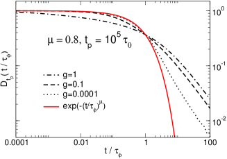
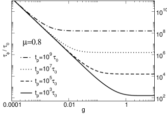
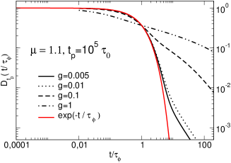
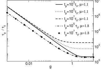
Figure 2: Dephasing factor and $\tau_{\phi}$ obtained by numerical inversion of (8) for $\mu<1$ (left) and $1<\mu<2$ (right). For weak coupling, $g<g_{c}(t_{\mathrm{p}})$, the decay is exponential for $t<\tau_{\phi}$. For times $t>\tau_{\phi}$ $(\mu<1)$ - $t\gg\tau_{\phi}$ $(1<\mu<2)$ - and for strong coupling the decay is algebraic. For strong coupling and $\mu<1$ the dephasing time exhibits a $t_{\mathrm{p}}$-dependence, which disappears as $\mu$ increases to higher values. Note the explicit $t_{\mathrm{p}}$-dependence of the critical coupling $g_{c}$ in the case $\mu<1$.

We now turn to a discussion of the results we can derive exactly from Eq.(8). As discussed above, the dephasing scenario differs qualitatively and quantitatively depending on the value of $\mu$. Generally, two regimes appear as a function of the coupling constant $g$, separated by a critical coupling constant $g_{c}$: While the dephasing time depends on $g$ in the weak coupling regime, $g<g_{c}$, it saturates for $g>g_{c}$ as a function of $g$ (see Fig. 2). As expected, it turns out that the critical coupling strength $g_{c}$ is of order 1 for the Poissonian class $(\mu>2)$ as well as for $1<\mu<2$. However, in the case $\mu\leq 1$, we find that the range of the strong coupling regime increases with the age of the noise, i.e. $g_{c}$ decreases as a function of $t_{\mathrm{p}}$: $g_{c}(t_{\mathrm{p}})=\lambda(\mu)(\tau_{0}/t_{\mathrm{p}})^{\mu/2}$. This implies that any qubit surrounded by a noise with $0<\mu<1$ will eventually end up in the strong coupling regime.

In the following we will discuss in detail the decay of $D(t_{\mathrm{p}},t)$ as a function of $t$ and the scaling laws of $\tau_{\phi}$ as functions of $g$ for the three different classes of $\mu$ and for both weak and strong coupling. In particular, we will compare our results with those for the Poissonian class. For $\mu>2$, $H_{t_{\mathrm{p}}}(\tau)\simeq P(\tau)$ and from (8) $D(t_{\mathrm{p}},t)\simeq D(0,t)$. As expected, after a transcient regime ($t_{p}\lesssim\tau_{0}$), $D(t_{\mathrm{p}},t)$ becomes independant of $t_{\mathrm{p}}$. The results of [5, 6] for a single fluctuator are then recovered for the Poissonian class.

For $1<\mu<2$, strong corrections with respect to the Poissonian class $(\mu>2)$ occur in the strong coupling regime, $g>1$. In that regime, the decay law of $D(t_{\mathrm{p}},t)$ is no longer an exponential but becomes algebraic $D(t_{\mathrm{p}},t)\simeq[\tau_{0}/(\tau_{0}+t)]^{\mu-1}-[\tau_{0}/(\tau_{0}+t+t_{\mathrm{p}})]^{\mu-1}$. The dephasing time thereby exhibits an explicit $t_{\mathrm{p}}$-dependence, $\tau_{\phi}\simeq\tau_{0}[1/e+(\tau_{0}/t_{\mathrm{p}})^{\mu-1}]^{-1/(\mu-1)}$. Note that this $t_{\mathrm{p}}$ dependence is only important for values of $\mu$ close to one and disappears as $\mu$ approaches higher values (see Fig. 2). For weak coupling, $g<1$, the initial decay of $D(t_{\mathrm{p}},t)$ is very well described within a Gaussian approximation (second cumulant expansion). The decay is exponential, $D(t_{\mathrm{p}},t)=\exp(-t/\tau_{\phi})$, and $\tau_{\phi}$ scales as $\tau_{\phi}\simeq\tau_{0}g^{-2}$. Corrections with respect to Poissonian class are only subdominant for $t\lesssim\tau_{\phi}$ and disappear as $\mu$ increases to higher values. However, for times large compared to the dephasing time, $t\gtrsim\tau_{\phi}\log(\tau_{\phi}/\tau_{0})$, the above Gaussian approximation breaks down and the decay crosses over to a much slower power law (see Fig. 2).

In the case of $0<\mu<1$, the decay of coherence differs considerably from the Poissonian class in all regimes, due to the absence of a characteristic time scale in the waiting times distribution. For weak coupling $g<g_{c}(t_{\mathrm{p}})$ the decay for $t\lesssim\tau_{\phi}$ is accurately described by an exponential, $D(t_{\mathrm{p}},t)\simeq\exp[-(t/\tau_{\phi})^{\mu}]$ with $\tau_{\phi}=\tau_{0}A(\mu)g^{-2/\mu}$. Dephasing is therefore insensitive to the preparation time $t_{\mathrm{p}}$. This result can be recovered using the previously mentionned Gaussian approximation. However, we emphasize the anomalous scaling of $\tau_{\phi}$ as a function of $g$ (see Fig. 2). But $D(t_{\mathrm{p}},t)$ is not fully described within this approximation. First of all, even at weak coupling, the Gaussian approximation breaks down for times $t>\tau_{\phi}$. In this regime, the exponential decay is replaced by a much slower algebraic one: $D(t_{\mathrm{p}},t)\simeq B(\mu)~{}(t/\tau_{\phi})^{-\mu}$. This new behavior can be understood by noting that in this case and for $t>\tau_{\phi}$ $D(t_{\mathrm{p}},t)\simeq D(t_{\mathrm{p}},\tau_{\phi})~{}\Pi_{0}(\tau_{\phi},t-\tau_{\phi})\simeq(t/\tau_{\phi}-1)^{-\mu}$ . The second term of (7) corresponds to the anomalous random walk spreading of the phase $\Phi$: it leads to the exponential decay (see above) which is subleading beyond $\tau_{\phi}$. Hence, the leading term corresponds to the contribution of the noise configurations that did not change between $\tau_{\phi}$ and $t$. This situation of a main contribution induced by rare configurations is analogous to the physics of Griffiths singularities in disordered systems. In the strong coupling regime $g>g_{c}(t_{\mathrm{p}})$, $D(t_{\mathrm{p}},t)$ is dominated by the first term of Eq.(7). In this limit, the distribution of the phase of the qubit starts spreading over $[0,2\pi]$. Hence, most noise configurations produce a vanishing contribution to $D(t_{\mathrm{p}},t)$ and the whole average is dominated by those noise configurations that do not evolve during the experiment. The physics of this strong coupling regime is closely related to the physics of mean-field trap models of glassy materials[13], since the difference between quenched and annealed disorder is irrelevant in this case. The dephasing time then saturates as a function of $g$ and becomes proportional to $t_{\mathrm{p}}$ as seen in Fig. 2. Note that, at strong coupling, the Gaussian approximation breaks even down for short times and the decay of $D(t_{\mathrm{p}},t)$ is algebraic: it decays as $D(t_{\mathrm{p}},t)\simeq 1-\sin(\pi\mu)/(\pi\mu)(t/t_{\mathrm{p}})^{1-\mu}$. For longer times, $t>t_{\mathrm{p}}$, it crosses over to a much slower decay, $D(t_{\mathrm{p}},t)\simeq(t_{\mathrm{p}}/t)^{\mu}$.

Finally, in the marginal case $\mu=1$ of pure $1/f$ noise the above analysis is confirmed qualitatively. We mainly find logarithmic corrections to the above results, e.g. the critical coupling scales as $g_{c}(t_{\mathrm{p}})=\left[2(\tau_{0}/t_{\mathrm{p}})\ln(t_{\mathrm{p}}/\tau_{0})\right]^{1/2}$. For weak coupling, $g<g_{c}(t_{\mathrm{p}})$, the dephasing time is insensitive to $t_{\mathrm{p}}$ and scales as $\tau_{\phi}\simeq 2\tau_{0}\left|\ln g\right|/g^{2}$, whereas for strong coupling it depends algebraically on $t_{\mathrm{p}}$.

In summary, we have studied decoherence of a qubit due to the noise generated by a slow collective environment. Within a simple phenomenological model, we have derived exact expressions for the dephasing factor in various regimes. The crucial consequences of the nonstationarity of the noise are first the appearance of a history dependent coupling $g_{c}(t_{\mathrm{p}})$ which separate the weak and strong coupling regimes and, second, a non exponential decrease of the dephasing factor $D(t_{\mathrm{p}},t)$. Depending on the broadness ($\mu$) of the distribution of relaxation times of the environment, this nonexponential decay appears either before ($\mu<1$) or after $\tau_{\phi}$, but is a clear signature of the nonstationarity of the noise (i.e. $\mu<2$ in our model). In a more refined description of a collective noise source consisting of a collection of coupled clusters, we expect the nonstationarity of the dephasing to be related to the number of contributing clusters. Similarly to the studies of Paladino et al. [5] for usual telegraphic fluctuators, the nonstationary dephasing in our model will survive provided the phase $\Phi(t_{\mathrm{p}},t)$ is dominated by a few strongly coupled slow clusters. In the opposite limit of many contributing clusters, the usual Gaussian stationary dephasing should be recovered. Thus the search for such nonstationarity in the dephasing of simple solid state qubits would be of main interest for the correct characterization of the source of $1/f$ noise in these samples. Note however that dephasing is experimentally studied by repeated interference experiments without noise reinitialization in between. The dephasing is then characterized by a time-average instead of the average over configurations $D(t_{\mathrm{p}},t)$. In the case of a nonstationary noise these two expressions will differ (non ergodicity for $0<\mu\leq 1$) and special care should be given in analyzing the experimental results.

J. Schriefl thanks Yu. Makhlin for very useful discussions. P. Degiovanni thanks the Institute for Quantum Computing (Waterloo) and Boston University for support and hospitality during completion of this work.

References

- [1] Yu. Makhlin, G. Schön, A. Shnirman, Rev. Mod. Phys. 73, 357 (2001)
- [2] Y. Nakamura, Yu.A. Pashkin, T. Yamamoto, J.S. Tsai, Phys. Rev. Lett. 88, 047901 (2002).
- [3] Yu. Makhlin and A. Shnirman, Phys. Rev. Lett. 92, 178301 (2004)
- [4] M.B. Weissman, Rev. Mod. Phys. 60, 537 (1988).
- [5] E. Paladino et al., Phys. Rev. Lett 88, 228304 (2002).
- [6] Y. M. Galperin, B. L. Altshuler, and D. V. Shantsev, cond-mat/0312490
- [7] J.L. Black and B.I. Halperin, Phys. Rev. B 16, 2879 (1977)
- [8] Notice that these couplings were already present in Ref.[6] on dephasing, but treated approximately within the framework of spectral diffusion[7].
- [9] C.C. Yu and A.J. Leggett, Comments Condes. Matter Phys. 14, 231 (1988)
- [10] S. Ludwig et al., Phys. Rev. Lett. 90 105501 (2003)
- [11] Note that the physics associated with huge degeneracy of the classical ground state should be irrelevant in such mesoscopic clusters.
- [12] For a single Poissonian fluctuator, nonstationary effects arise in the transcient regime of times smaller than .
- [13] J.-P. Bouchaud, J. Physique I 2, 1705 (1992).
- [14] J.W. Haus and K.W. Kehr, Phys. Rep. 150, 263 (1987).
- [15] W. Feller, An Introduction to probability theory and its applications, Vol. 1, Wiley & Sons (1962)