Quantum interference in nanofractals and its optical manifestation

Abstract

We consider quantum interferences of ballistic electrons propagating inside fractal structures with nanometric size of their arms. We use a scaling argument to calculate the density of states of free electrons confined in a simple model fractal. We show how the fractal dimension governs the density of states and optical properties of fractal structures in the RF-IR region. We discuss the effect of disorder on the density of states along with the possibility of experimental observation.

I Peculiarity of metallic nanofractals

Ramified structures are widely observed in nature at scales from the microscopic world up to the human size. They have been studied in various contexts and in different domains of science: biology, physics, chemistry, etc. Surface Science is one particular field where the ramified semi-metalrefLAC ; refLyon , semiconductorrefBorsella , metallicrefPallmer ; refShalaevBottet or dielectricMarkel ; refShalaev structures may range from the nanometric up to the micrometric sizes. The mean free path of electrons in metals is usually of the order of $10^{2}$-$10^{3}$ $nm$ depending on the kinetic energy. Therefore electrons propagating ballistically in metallic nanostructures may manifest essentially quantum behavior associated with strong interference of their De Broglie waves in contrast to the diffusiverefKhmelnitskii or hoppingShklovskii behavior intensively studied during the last decades. The combination of quantum ballistic motion and ramified geometry suggests to consider the interference of electrons in a fractal metallic structure confining their propagation.

Tree-like structures is a natural example of fractals. Results obtained for quantum particles moving on tree-like laticesrefDerrida , for the quantum localization in the framework of sparse random matrix modelsrefMirlin topologically similar to trees, and for quantum systems with tree-like hierarchy of interactionsLevitov have revealed a certain universality associated with such a topology, that persists in different physical situations. Therefore for tree-like fractals one can also expect a universality of the quantum properties related to their specific geometry. Moreover, the key property of fractal structures is the invariance under certain scaling transformations. Therefore considering quantum dynamics of electrons on fractal trees we take advantage of the scaling argumentsrefWilson . Note that it is equally important to study the properties of ensembles of isolated or interacting fractals placed together at a surface, since it is experimentally difficult to address a single nanometric object. Models of such ensembles might be also of interest for consideration of conductivity of thin filmsrefSaintGobain , heterogeneous catalysis of nanometer larger silver particlesrefCatalyst , quantum dot networksrefQuantumdots , and in other domains.

In this paper, we consider the simplest tree-like fractal with identical length of the branches at each generation and symmetric nodes as a support of ballistically propagating electrons. We introduce a single geometrical parameter $a$ which gives the ratio of branch lengths for successive generations. We shall see that this parameter is closely related to the fractal dimension of the tree. We show that the density of the one-electron states manifests a power law dependence on the momentum near zero energy with the power index being the fractal dimension. It is consistent with the resultrefMath for the low momentum asymptotic of Green functions in systems of fractal dimensionality. Note that this property is typical of fractals since linear objects of the same size do not have quantum states close to zero energy according to the Born-Sommerfeld quantization rule. We demonstrate the macroscopic manifestations of this power law in optical properties of surfaces covered by the nanometric ramified structures by calculating the reflectivity in the RF-IR frequency domain. Finally, with the help of a simple random matrix approachrefAkulin we consider the role of irregularities in fractal structures resulting from the statistical distribution of branch lengths and nodes asymmetries, that does not require to allow for the level-level correlations in the ballistic regime.

We formulate the problem in terms of the Green functions of a particle propagating along the fractal. We employ the momentum variable which is natural for consideration of the interference phenomena, whereas the energy dependence is given by the dispersion law $E=E(p)$ specific for each type of systems. It allows one to implement the results for any particular dependence of the particle energy on the momentum which are usually different for metals and for semiconductors: for a free particle $E=p^{2}/2m$, where $m$ is the mass of the particle, whereas for metals $E=v_{f}|p|$, where $v_{f}$ is the Fermi velocity. One-particle Green functions are obtained following the standard quantum field formalism widely developed in various textbooksrefAbrikosov . Quantum state density $g(p)$ and several other properties such as linear dipole response $R(\omega)$ or conductivity $\sigma(\omega)$ at a frequency $\omega$ can be found with the help of its retarded $\widehat{G}^{R}(E)$ and advanced $\widehat{G}^{A}(E)$ Green operators via the relationsrefEfetov

$$\begin{array}[]{c}g(p)=-\frac{1}{\pi}{\rm Im~{}Tr~{}}\widehat{G}^{R}(E)\\ R(\omega)={\rm~{}Tr~{}}\widehat{G}^{A}(E)\widehat{d}\widehat{G}^{R}\left(E+\omega\right)\widehat{d}\widehat{\rho}(p),\\ \sigma(\omega)={\rm~{}Tr~{}}\widehat{G}^{A}(E)\widehat{j}\widehat{G}^{R}\left(E+\omega\right)\widehat{d}\widehat{\rho}(p)\end{array}$$ (1)

where $\widehat{d}$ is the dipole moment operator, $\widehat{j}$ is the current operator, and $\widehat{\rho}$ is the density matrix. By the analogy to a photon propagating in a Fabri-Perot resonator, we can take into account only the coordinate parts $G(p,x,x^{\prime})$ of the Greens operators at a given energy $E(p)$ ignoring the resonant denominators $(E-E(p)+i0)$. The latter can be factored out during the consideration of the interference phenomena and have to be restored only at the last stage, prior to substitution to Eqs.(1). Note that in the case of ballistic propagation the coordinate part of the product $G^{A}(E)G^{R}\left(E+\omega\right)$ can be written in a single factor $G(p)$ depending only on the momentum $p=\omega.p_{E}^{\prime}$, where $p_{E}^{\prime}=1/v_{f}$, associated with the energy shift $\omega$. For $g(p)$, ${\rm Im}~{}R(\omega),$ ${\rm Re~{}}\sigma(\omega)$ the allowance for denominators yields the Dirac $\delta$-functions of energies which disappears after taking the trace. Therefore these parameters responsible for the absorption of electro-magnetic radiation can be calculated directly when we replace${\rm~{}}G^{A}G^{R}$ in Eqs.(1) by $G(p)$. The Kramers-Kronig relation then yields the dispersive parts ${\rm Re~{}}R(\omega)$ and ${\rm Im}~{}\sigma(\omega).$ In this paper we therefore call ”Green function” the coordinate part $G(p,x,x^{\prime})$ of $\widehat{G}^{A}(p_{f})\widehat{G}^{R}(p+p_{f})$.

For metals the density matrix is given by the Fermi step $\widehat{\rho}(p)=v_{f}n_{e}\Theta(-p)$ where $n_{e}$ is the electron state density in metal near the Fermi surface and the Fermi momentum is taken as a reference point. The dipole moment operator $\hat{d}$ in the momentum representation reads $\widehat{d}=ie\partial/\partial p$ where $e$ is the electron charge (we set $\hbar=1$), whereas the current operator $\widehat{j}$ is simply $pe/m$. Therefore Eq.(1) takes the form

$$\begin{array}[]{c}g(p)=\frac{1}{\pi}{\rm~{}Tr~{}}G(p)\\ {\rm Im}~{}R(\omega)=v_{f}e^{2}n_{e}\left.\frac{\partial}{\partial p}\right|_{p=0}{\rm~{}Tr~{}}G\left(p+\frac{\omega}{v_{f}}\right)\\ {\rm Re~{}}\sigma(\omega)=\frac{e^{2}n_{e}\omega}{mv_{f}}{\rm~{}Tr~{}}G\left(\frac{\omega}{v_{f}}\right)\end{array}$$ (2)

where we have taken into account the relation $\partial\Theta(p)/\partial p=-\delta(p)$. The trace operation now implies only summation over all closed trajectories in the coordinate space corresponding to a given momentum in complete analogy with the Fabri-Perot resonator.

II The model of fractal

We model a fractal by three trees with trunks joint in a node at the fractal center(Fig.1). Each of the trees starts with a trunk of length $L$ and is built by recursive attaching at each terminations two homothetical branches scaled by a factor $a$. The homothetical factor $a$ is the main parameter of the model. It governs all geometrical properties and in particular the fractal dimension which is the main physical parameter. For $a>1$ branches are longer at each step, whereas for $a<1$, branches are smaller as $n$ increases, which is always the case in our consideration as we shall see. Electrons propagate ballistically along the trunks and branches until they reach a node where three branches are attached symmetrically at the angle $2\pi/3$ as shown in Fig.1. Nodes scatter the electrons backwards and forward into the attached branches.

II.1 Nodes model

The branches joining a node have different length which depends on the index $n$ numerating the generation, that is the number of nodes which separates the branch from the fractal center. Two branches are of the length $L_{n}=a^{n}L$ whereas the branch closest to the trunk has the length $L_{n-1}=a^{n-1}L$. If we stop the development of the tree at a given $n=N$, the last rightmost branches have a length $L_{N}=a^{N}L$ and the total number of such branches is $2^{N}$.

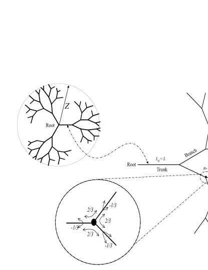
Figure 1: Model tree consisting of a trunk of length $L_{0}=L$ and successive adjunction of branches. At each generation $n$, two branches of length $L_{n}=a.L_{n-1}$ are attached to the previous branch. The scaling parameter $a$ governs the tree morphological properties, mass, length and fractal dimension. We restrict to $1/2<a<1$. The scattering matrix (Eq.4) couples incoming fluxes to outgoing ones. The fractal of radius $Z$ is built by attaching three identical trees to the root.

Having arrived at a node an electron either scatters into the two attached branches with equal (due to the symmetry) probability or returns back with a different probability. The node is formally described by a unitary $3\times 3$ scattering matrix $\hat{S}$ with the matrix elements $s_{j,j^{\prime}}$ coupling three outgoing probability amplitudes $\phi_{j}$ of the electron to the three incoming $\psi_{j}$ ones, where the marker $j$ assumes the values, $l$, $r$, and $b$ for the left-scattered, right-scattered, and the back-scattered amplitudes, respectively. The relation among the amplitudes reads

$$\left(\begin{array}[]{c}\phi_{b}\\ \phi_{r}\\ \phi_{l}\end{array}\right)=\left(\begin{array}[]{ccc}s_{bb}&s_{br}&s_{bl}\\ s_{rb}&s_{rr}&s_{rl}\\ s_{lb}&s_{lr}&s_{ll}\end{array}\right)\left(\begin{array}[]{c}\psi_{b}\\ \psi_{r}\\ \psi_{l}\end{array}\right)$$ (3)

Apart of the unitarity, the matrix $\hat{S}$ should satisfy two more requirements imposed by the node symmetry and by the long wave limit. The symmetry requirement implies that the probability amplitudes for the left- and the right-scattering given by the coefficients $s_{rb}$ and $s_{lb}$ respectively, are equal. Moreover, the symmetry with respect of the node rotation at the angle $2\pi/3$ implies that all other off-diagonal coefficients also have the same value. We also assume that no quantum defect is associated with the scattering at the node. In the long wave limit it implies that no phase shift is introduced during the scattering process, and hence all the parameters $s_{j,j^{\prime}}$ are real. These three requirements together yield

$$\hat{S}=\left(\begin{array}[]{ccc}-\frac{1}{3}&~{}\frac{2}{3}&~{}\frac{2}{3}\\ ~{}\frac{2}{3}&-\frac{1}{3}&~{}\frac{2}{3}\\ ~{}\frac{2}{3}&~{}\frac{2}{3}&-\frac{1}{3}\end{array}\right)$$ (4)

as the only choice for the scattering matrixrefTexier .

II.2 Scaling factor and the fractal dimension

Now we relate the typical length $L$ of the system and the scaling factor $a$ with the fractal dimension employing the self similarity aspect of the problem. In fact, in the general case $L$ is not the only typical length scale in the problem. The homothetical factor $a$ governs most of the advanced morphological properties of the model tree. The total length $Z_{N}$ of the tree with truncated branches of $N+1$-th generation reads

$$Z_{N}=\sum\limits_{k=0}^{N}L_{k}=\sum\limits_{k=0}^{N}a^{k}L=L\frac{1-a^{N+1}}{1-a}$$ (5)

This expression imposes a first limit on $a$ : for $0<a<1$ the length $Z_{N}$ converges to a finite value

$$Z=\frac{L}{1-a}$$ (6)

whereas for $a\succeq 1$ it diverges. We consider the fractals of a finite size only. Actually, the radius of a tree is given by a more complicated expression and should take into account the geometrical arrangement of the branches with $2\pi/3$ angle between them. The exact calculation for the diameter gives $D_{N}=L(2+a)(1-a^{N+1})/(1-a^{2})$ which also converges when $N\rightarrow+\infty$ for $a<1$ to the value $D=L(2+a)/(1-a^{2})$.

The mass $M_{N}$ of the tree that is the sum of the lengths of all branches is given as

$$M_{N}=\sum\limits_{k=0}^{N}2^{k}L_{k}=\sum\limits_{k=0}^{N}2^{k}a^{k}L=\frac{1-(2a)^{N+1}}{1-2a}L$$ (7)

which converges to $M=L/(1-2a)$ for $a<1/2$ and diverge for $a>1/2$. We are interested in the regime where the mass of the fractal is infinite, and therefore $a$ ranges from $1/2$ to $1$.

The model fractal has the same fractal dimension as its consisting trees. The fractal dimension of a tree is given by a standard evaluation refMandelbrot which is now widely used. It implies the calculation of the minimum number $N(\varepsilon)$ of disks of diameter $\varepsilon$ needed to completely cover the whole tree. In a fractal structure, gradual decreasing of $\varepsilon$ reveals new details causing $N(\varepsilon)$ to vary non trivially as $\varepsilon^{-D_{h}}$ where $D_{h}$ defines the so called Hausdorff-Besicovitch fractal dimension.

Let us implement this definition in our case of tree-like fractal. In order to find the number $N(\varepsilon)$ of $\varepsilon$-sized disks required for covering the tree we make use of the scaling arguments. Let us take the infinite tree and applying to it the homothetical factor $a$. One obtain another tree which also has the same infinite structure but starts with a smaller trunk of length $aL$. This $a$-contracted tree can be considered as an element of the original tree, namely its first generation branch with all the branches of subsequent generations attached. The size of the discs covering this branch is apparently $a$ times smaller compared to original discs of the radius $\varepsilon$. When we attach two $a$-contracted trees to a trunk of length $L$ we recover the original form of our fractal with branches covered by $2N(\varepsilon)$ discs of radius $a\varepsilon$. One requires $L/a\varepsilon$ additional discs to cover the trunk. We therefore obtain the equation

$$N(\varepsilon a)=2N(\varepsilon)+\frac{L}{a\varepsilon}$$ (8)

determining an asymptotic behavior of $N(\varepsilon)$ for $\varepsilon\rightarrow 0$.

We look for the solution of Eq.(8) in the power-law form $N(\varepsilon)\sim\varepsilon^{-\alpha}$ with $\alpha>1$. It implies that the second term in the right hand side of Eq.(8) can be omitted with respect to the first term as $\varepsilon\rightarrow 0$, and we arrive at $(a\varepsilon)^{-\alpha}=2(\varepsilon)^{-\alpha}+o(\varepsilon^{-\alpha})$. It yields

$$\alpha=-\frac{\ln 2}{\ln a}$$ (9)

which is the well-known Hausdorff-Besicovitch fractal dimension of a self similar recursively built fractalrefMandelbrot . Equation (9) gives fractal dimension greater than $1$ in the case $a>1/2$ corresponding to an infinite mass $M$. We also restrict ourselves to the case $a<1$ corresponding to a finite size $Z$ of fractals. In this regime the spectral peculiarities typical of such structures manifest themselves in the most interesting way.

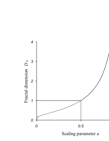
Figure 2: Fractal dimension $D_{h}$ as function of the scaling parameter $a$. For $0<a<1/2$ the tree has a finite mass and its fractal dimension is dominated by the trunk : $D_{h}=1$. For $1/2<a<1$ the mass is infinite whereas its length remains finite : $D_{h}=\alpha=-\ln(2)/\ln(a)$

III Green functions and quantization of the fractal states

The Green functions $G(p)$ generally given by the Feynmann path integral can be found for the particular case of a tree-like fractal structure from recurrent relations formulated in terms of the Green function of a free one dimension particle $G_{o}(p)=\Theta(x-x^{\prime})\exp[ip(x-x^{\prime})]$ propagating along the branches and the scattering conditions Eq.(3) at the nodes. We derive a recurrent relation for these functions and thereby determine the spectrum of the eigen state density.

III.1 Recurrent relations

The idea of derivation of the recurrent relations is illustrated in Fig.3a). By $X_{n}(p)$ we denote the unknown exact Green function for the particle leaving a chosen node of $n$-th generation and returning back after multiple scattering in all the variety of nodes of subsequent generations connected to the chosen node. Then the Green function $X_{n-1}$ of the previous generation can be considered as a result of the free propagation of the particle towards the $n$-th node followed by the multiple scattering at this node resulting in the direct back scattering $s_{bb\text{ }}$and the scattering to the attached branches followed by the multiple returns and back-scattering in the nodes and branches of the subsequent generations. One finds the result of all these multiple scattering events by considering the relation Eq.(3) among the incoming $\phi$ and outgoing $\psi$ amplitudes with the allowance for the fact that they are related by the condition

$$\psi_{l,r}=X_{n}(p)\phi_{l,r}$$ (10)

which holds by the definition of Green functions.

The free propagator $G_{o}(p)$ gives the relation

$$\widetilde{\psi}=\exp[ipLa^{n}]\phi_{b};\quad\psi_{b}^{in}=\exp[ipLa^{n}]\widetilde{\phi}$$ (11)

between the amplitudes $\psi_{b}$ and $\phi_{b}$ of the waves incoming to and outgoing from the node $n$ along the branch attached to the node $n-1$ and the amplitudes $\widetilde{\phi}$ and $\widetilde{\psi}$ of the waves outgoing from and incoming to the latter. Here we do not specify whether $\widetilde{\psi}^{in,out}$ corresponds to the right scattered or to the left scattered amplitudes at the node $n-1$ since the relation are identical for both cases. The scattering matrix Eq.(4) and the condition $\widetilde{\psi}=X_{n-1}\widetilde{\phi}$ together with Eqs.(3,10,11) yield the exact recurrence relation for the Green functions

$$X_{n-1}(p)=\exp[2ipLa^{n}]\frac{1-3X_{n}(p)}{X_{n}(p)-3}$$ (12)

Equation (12) maps the Green function $X_{n}(p)$ of a $n$-th node to the Green function $X_{n-1}(p)$ corresponding to a node of the previous generation. As we are interested in the high $n$ behaviour, this equation has to be inverted to obtain the expression of $X_{n}(p)$ as function of $X_{n-1}(p)$. Changing the $n$ index to $n+1$ we have

$$X_{n+1}(p)=\frac{\exp[2ipLa^{n+1}]+3X_{n}}{3\exp[2ipLa^{n+1}]+X_{n}(p)}$$ (13)

that we make use in Fig.3b) for $p=0$.

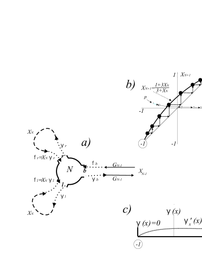
Figure 3: Recurrent relations for the Green functions. (a) A Green function $X_{N-1}$ attached to a parent node consists of a free propagation $G_{0}$ followed by the scattering in the node of the next generation and back propagation. Amplitudes by the outgoing and incoming waves in each branch differ by the factor $X_{N-1}$. (b) The mapping corresponding to Eq.(13) in the long wave limit $p=0$ has two stationary points. One corresponds to a regular back-scattering with the phase shift $-\pi$, whereas the other does not yield any phase shift and gives rise to the essentially fractal domain of the spectrum near zero energy. (c) Boundary conditions at nodes corresponding to the stationary point $-1$ (left), and $+1$ (right).

This mapping Eq.13 has two stationary points $X_{st}=\mp 1$. Both of them have physical meaning. The negative sign corresponds to the regular situation when the reflection of the wave function from a node occurs with a phase shift $-\pi$ exactly in the same way as the reflection from an infinite vertical barrier implied by the boundary condition $\psi=0.$ The positive sign corresponds to a free border $\psi_{x}^{\prime}=0$ when the wave goes through the node and returns back with no phase shift, as shown in Fig.3c). The latter case changes the quantization rule for a particle moving in a branch confined by such nodes from both sides allowing the eigen states at zero energy that do not exist for the regular confinement. Vicinity of this stationary point gives rise to a specifically fractal domain of the energy spectrum at small values of the energies and momenta.

III.2 Scaling

Now we make use of the scaling arguments and find the Green function in the long wave asymptotic and large $n$. The scaling assumption implies that $X_{n-1}(p)=X_{n}(ap)$, which means that the Green functions $X(x)$ corresponding to the branches of any generation are functionally identical and differ only by scaling of the argument $x=a^{n}p$. Therefore in the long wave asymptotic where $exp(2IpLa^{n})\rightarrow 1$ Eq.(12) takes the form

$$X(x)=\frac{1-3X(ax)}{X(ax)-3}$$ (14)

of a functional equation, where we have employed a small dimensionless argument $x=Lp$ instead of $p$.

This equation has an exact solution

$$X(x)=\frac{1-x^{\alpha}}{1+x^{\alpha}}$$ (15)

with $\alpha$ given by Eq.(9) and yields an asymptotic expression

$$X_{n}(Lp)=\frac{1-(a^{n}Lp)^{\alpha}}{1+(a^{n}Lp)^{\alpha}}.$$ (16)

Equation (16) holds for small arguments. However, even for a large values of $x=Lp$ or small $n$ an accurate numerical approximation can be obtained with the help of few iterations of the exact recurrent relation Eq.12. For low $p$ and for $a=2/3$, with Eq.15 as a starting point, say $n=10$ iterations of Eq.12 gives a good approximation within $1$% compared to the exact solution Eq.16.

III.3 Quantization and state density

Now we are in the position to perform the quantization of the particle motion on the entire fractal and determine the density of the energy eigen states. For the purpose we consider the root node at the center of the fractal with three trunks attached and calculate contributions of all closed trajectories that start and end in a point of one of these trunks close to the node. The trajectory sum starts with the zero length trajectory which gives the contribution $1$. The trajectory first going to the trunk and returning back gives the contribution $X_{0}(Lp)$, whereas the contribution of the trajectory which first goes to the node is $B=(1-3X_{0})/(X_{0}-3)$ according to Eq.(12). The trajectories of the second order give $X_{0}B$ and $BX_{0}$ whereas the third order results in $X_{0}BX_{0}$ and $BX_{0}B$. The overall sum reads

$$\begin{array}[]{c}{\rm~{}Tr~{}}G(p)=1+X_{0}+B+X_{0}B+BX_{0}+..\\ =\frac{(1+X_{0})(1+B)}{1-BX_{0}}=\frac{2}{3}\frac{1+X_{0}}{1-X_{0}}.\end{array}$$ (17)

as it follows from summation of the geometric series.

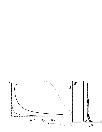
Figure 4: Density of states for different fractal dimensions $\alpha=1.18$ corresponding to $a=5/9$ (solid line), $\alpha=1.41$ corresponding to $a=11/18$ (dash-dot line), and $\alpha=1.71$ corresponding to $a=6/9$ (dashed line), calculated with the help of Eq.(17) where $X_{0}$ has been obtained from Eq.(16) after 10 iterations of Eq.(12). The fractal diameter is the same for all fractal dimensions. Vertical lines shows positions of the levels in a one dimensional potential well of a width equal to the fractal diameter.

In the long wave limit, injecting Eq.(15) into Eq.(17) we find

$${\rm~{}Tr~{}}G(p)=\frac{2}{3}(Lp)^{-\alpha},$$ (18)

which shows that at small energies the density of fractal energy eigen states follows the power law dependence on the momentum with the power index given by the Hausdorff-Besicovitch fractal dimension. In Fig.4 we illustrate the difference between the fractal spectrum found from Eq.(17) and the spectrum of a one dimensional particle moving in the potential well of the width $2Z=2L/(1-a)$ suggested by Eq.(6) for the fractal diameter. One clearly sees that the fractal boundary conditions at the nodes corresponding to the stationary point $X=1$ of mapping Eq.(14) result in the appearance of the spectrum near zero energy, where the potential well does not have eigenstates.

IV Nanofractal response to IR-RF field

Let us consider now the optical response of the nanofractals calculating the reflectivity of a transparent support surface covered by fractals as a function of the incident field frequency. We start with the case of isolated fractals each of which independently contribute to the reflectivity. The typical frequency domain can be estimated as the inverse of the typical time of flight of an electron across the fractal given by the Fermi velocity divided by the fractal size $Z$ Eq.(6), which for the fractalsrefLAC of $100nm$ corresponds to the THz frequency domain that is far IR or short RF radiation. Then we consider the case of ”merging” fractals, when the neighboring fractals irregularly placed at the surface can interact with capacitor-like connections via their most closely approaching terminations.

IV.1 Isolated nanofractals

The Maxwell equation

$$\frac{\partial^{2}}{\partial x^{2}}{\bf E}-\frac{\omega^{2}}{c^{2}}{\bf E}=\frac{4\pi}{c^{2}}\delta(\frac{x}{b})\left[i\omega\sigma_{s}(\omega)+\frac{\omega^{2}}{c}R_{s}(\omega)\right]{\bf E}$$ (19)

for a plane electromagnetic wave ${\bf E}$ incident normally to a surface covered by isolated fractals at $x=0$ allows one to find an intensity of the reflected field ${\bf E}_{r}$ provided the specific conductivity $\sigma_{s}(\omega)$ and the specific dipole susceptibility $R_{s}(\omega)$ of a unit surface area are known. The inhomogeneities of the surface have to be much smaller compared to the wavelength of the wave and the thickness $b$ of the fractal layer. For a wave incident at an angle to the surface the same equation is valid for the tangent component of the field, whereas the normal component is not affected by the layer of the fractals. The continuity condition for the tangent field and the jump of its derivative across the surface

$$\begin{array}[]{c}{\bf E}+{\bf E}_{r}={\bf E}_{t}\\ \frac{\omega}{c}\left({\bf E}-{\bf E}_{r}-{\bf E}_{t}\right)=\frac{4\pi b}{c^{2}}\left[i\omega\sigma_{s}(\omega)+\frac{\omega^{2}}{c}R_{s}(\omega)\right]{\bf E}_{t}\end{array}$$ (20)

yield the relation

$$\begin{array}[]{c}\frac{{\bf E}_{r}}{{\bf E}}=\frac{-2\pi b\left[ic\sigma_{s}(\omega)+\omega R_{s}(\omega)\right]}{c^{2}+2\pi\left[ic\sigma_{s}(\omega)+\omega R_{s}(\omega)\right]}\\ \simeq\frac{-2\pi b}{c^{2}}\left[ic\sigma_{s}(\omega)+\omega R_{s}(\omega)\right]\end{array}$$ (21)

for the ratio of the reflected and the incident field amplitudes.

Equations (2,18) yield

$$\begin{array}[]{c}{\rm Im}~{}R(\omega)=-N_{f}\alpha v_{f}^{2}\frac{e^{2}n_{e}}{\omega}\frac{2}{3}(\frac{L\omega}{v_{f}})^{-\alpha}\\ {\rm Re~{}}\sigma_{s}(\omega)=\frac{2e^{2}n_{e}\omega}{3v_{f}m}N_{f}{\rm~{}}(\frac{L\omega}{v_{f}})^{-\alpha}\end{array}$$ (22)

where $N_{f}$ is the number of fractals per unit area. We replace the product $N_{f}n_{e}$ by the specific density of states $n_{s}$ of the fractal material near the Fermi surface multiplied by the total volume ${\cal V}$ of the material deposited per unit surface, express the trunk size $L=Z\left(1-a\right)$ in terms of the typical fractal size $Z$ Eq.(6) and the fractal dimension $\alpha$ Eq.(9), and substitute $\sigma/v_{f}\lambda$ instead of the product $n_{s}e^{2}$ where $\sigma$ is the residual conductivityrefLifPit and $\lambda$ is the electron mean free path in bulk metal. In the last replacement we assume that $n_{s}=N_{el}/p_{f}v_{f}$ where $N_{el}$ is the density of the metal electrons. We arrive at

$$\begin{array}[]{c}{\rm Im}~{}R_{s}(\omega)=-\frac{4\sigma\alpha{\cal V}v_{f}}{3\omega\lambda\left(2^{1/\alpha}-1\right)^{\alpha}}(\frac{Z\omega}{v_{f}})^{-\alpha}\\ {\rm Re~{}}\sigma_{s}(\omega)=\frac{4\sigma{\cal V}\omega}{3\lambda mv_{f}^{2}\left(2^{1/\alpha}-1\right)^{\alpha}}{\rm~{}}(\frac{Z\omega}{v_{f}})^{-\alpha}.\end{array}$$ (23)

Non-analytical behavior of these dependencies at $\omega=0$ does not allow one to determine the dispersive parts ${\rm Re}~{}R_{s}(\omega)$ and ${\rm Im~{}}\sigma_{s}(\omega)$ from the Kramers-Kronig relations. However the latter should be of minor importance provided the transparent material supporting the fractal at its surface has a refraction index $r$ different from $1$. In the latter case

$$\frac{{\bf E}_{r}}{{\bf E}}\simeq\frac{{\cal V}b\sigma}{c\lambda}\frac{8i\pi(Z\omega/v_{f})^{-\alpha}}{3\left(2^{1/\alpha}-1\right)^{\alpha}}\left[\frac{\alpha v_{f}}{c}-\frac{\omega}{p_{f}v_{f}}{\rm~{}}\right]+\frac{1-r}{1+r}.$$ (24)

The simplest possible way to find the missing parts is to take an analytical continuation of Eq.(23) to the complex plane such that $g(Z\omega/v_{f})\sim\omega^{-\alpha}$ vanishes at the negative part of the real axis.

IV.2 Ensemble of nanofractals

When the size of the fractals becomes larger than the inter-fractals distance, the model of isolated fractals fails, since the dipole approximation for the response is not any longer valid. In the same time, allowing for the contribution related to the conductivity we have to take into account the points of the closest approach of neighboring fractals, where the potential difference experience large changes. These domains work as capacitors that assume the main part of the dipole activity of the system. When the ramified structures are randomly distributed on the surface but not yet result in the electric current percolation, as it is the case for the experimental workrefLAC for instance, the fractal ensembles conform the Dykhne modelrefDykhne . Formulated for a two-phase random conducting surface with the conductivities $\sigma_{1}$ and $\sigma_{2}$ different for different phases this model yields the macroscopic conductivity $\sigma_{eff}=\sqrt{\sigma_{1}\sigma_{2}}$ which immediately suggests

$$\sigma_{eff}=\left[\frac{4\sigma{\cal V}\omega}{3\lambda mv_{f}^{2}\left(2^{1/\alpha}-1\right)^{\alpha}}{\rm~{}}(\frac{Z\omega}{v_{f}})^{-\alpha}\frac{i\omega b^{2}}{Zd}\right]^{1/2}$$ (25)

for the effective conductivity of the fractals covering the surface. Here we have assumed that the capacitors of a plate size $b$ separated by a mean shortest inter-fractal distance $d$ are subjected to the potential difference $Z{\bf E}$ accumulated on the distance of the fractal size $Z$.

Substitution of Eq.(25) to Eq.(21) yields

$$\frac{{\bf E}_{r}}{{\bf E}}\simeq i\frac{2\pi\omega b^{2}}{cv_{f}}\left[\frac{\sigma{\cal V}}{6\lambda mZd\left(2^{1/\alpha}-1\right)^{\alpha}}{\rm~{}}\right]^{\frac{1}{2}}\left(\frac{Z\omega}{v_{f}}\right)^{-\frac{\alpha}{2}}+\frac{1-r}{1+r}$$ (26)

where we have omitted the real part of the effective conductivity as small relative to the support contribution.

IV.3 Random fractals

Thus far we have been considering the model of an ideal fractal with a high symmetry and an exponential variation of the branch lengths with generation number. In order to get an idea of how close can be such a model to the reality we now consider an ensemble of irregularly distorted fractals. The simplest way to model the random distortion is to treat it as a perturbation of the fractal Hamiltonian by a random matrix with a given mean square $\left\langle V^{2}\right\rangle$ of the matrix elements. The transformation rule

$$\widetilde{\widehat{G}}(E)=\widehat{G}(\widetilde{E}(E))$$ (27)

$$E=\widetilde{E}+\left\langle V^{2}\right\rangle{\rm Tr}\widehat{G}(\widetilde{E})$$ (28)

suggested by one of the authorsrefAkulin as a simple way to solve the PasturrefPastur equation describing such a perturbation. Eq.(27) relates the ensemble averaged perturbed Green function $\widetilde{\widehat{G}}(E)$ with the unperturbed one $\widehat{G}(E)$ depending on a transformed argument $\widetilde{E}(E)$. The transformation $\widetilde{E}(E)$ follows from the solution of a nonlinear algebraic equation (Eq.(28)) which allows one to find $\widetilde{E}$ for each $E$ selecting from many possible solutions the one continuously changing from $-\infty$ to $\infty$ for $E$ varying in this interval. By the same replacement of the argument one can obtain all other linear properties of the randomly perturbed system.

Comparing Eqs.(1,2) and Eq.(18) with the allowance of the condition $g(E<0)=0$ one finds an expression

$${\rm~{}Tr~{}}\widehat{G}(E)=-g_{0}\frac{1}{{\rm Im(-1)^{-\alpha}}}(\frac{-LE}{v_{f}})^{-\alpha}$$ (29)

consistent with the state density Eq.(1) for both the positive and the negative energies. The constant $g_{0}$ enters as a cofactor of the other unknown quantity $\left\langle V^{2}\right\rangle$ and both factors together form a single energy parameter $W=g_{0}\left\langle V^{2}\right\rangle$ responsible for the strength of the random perturbation. We substitute Eq.(6,9,29) to Eq.(28) and obtain

$$E=\widetilde{E}+\frac{W}{{\rm\sin}\pi\alpha}\left[\frac{-Z(1-2^{-1/\alpha})\widetilde{E}}{v_{f}}\right]^{-\alpha}$$ (30)

One sees that by introducing an energy scaling factor $E={\cal E}F$ with $F=\left(Z(1-2^{-1/\alpha})/v_{f}\right)^{\alpha/(\alpha+1)}W^{-1/(\alpha+1)}$ equation (30) can be reduced to the form

$${\cal E}=\widetilde{{\cal E}}+\frac{(-\widetilde{{\cal E}})^{-\alpha}}{{\rm\sin}\pi\alpha}$$ (31)

which does not contain parameters other than the fractal dimension.

In order to find the universal dependencies $\widetilde{{\cal E}}({\cal E,}\alpha)$ there is no need to solve the equation (31). After the replacement $\widetilde{{\cal E}}=-\kappa e^{i\theta}$, one eliminates $\kappa$ employing the fact that ${\cal E}$ is real and finds the dependence $\widetilde{{\cal E}}({\cal E})$ in a parametric form

$$\begin{array}[]{c}\widetilde{{\cal E}}\left(\theta\right)=-e^{i\theta}\left(\frac{-\sin\alpha\theta}{\sin\theta{\rm\sin}\pi\alpha}\right)^{1/(1+\alpha)}\\ {\cal E}\left(\theta\right)=-\left(\frac{-\sin\alpha\theta}{\sin\theta{\rm\sin}\pi\alpha}\right)^{\frac{1}{1+\alpha}}\cos\theta+\left(\frac{-\sin\alpha\theta}{\sin\theta{\rm\sin}\pi\alpha}\right)^{\frac{-\alpha}{1+\alpha}}\frac{\cos\alpha\theta}{{\rm\sin}\pi\alpha}.\end{array}$$ (32)

The imaginary part of $\widetilde{{\cal E}}({\cal E},\alpha)/\pi$ shown in Fig.5

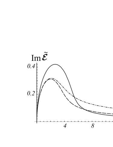
Figure 5: Universal forms of the quantum state density profiles for randomly perturbed fractals with the fractal dimensions $\alpha=1.18$ (solid line), $\alpha=1.41$ (dash-dot line), and $\alpha=1.71$ (dashed line). These profiles do not depend on the size of the perturbation which results only in scaling of the energies.

as a function of the energy ${\cal E}$ for different fractal dimensions $\alpha$ yields the shape of the state density $g_{\alpha,W}(E)=F{\rm Im}\widetilde{{\cal E}}(E/F,\alpha)/\pi$ which for the case of irregular fractals should replace the factor ${\rm Tr}G(p)/\pi=\frac{2}{3\pi}[Z\omega/v_{f}(2^{1/\alpha}-1)]^{-\alpha}\sim{\cal E}^{-\alpha}$ in the expression Eq.(4) as well as in Eqs.(23) for the dipole response and the conductivity and in Eq.(26) for the effective conductivity of a disordered surface. It yields

$${\rm Im}\frac{{\bf E}_{r}}{{\bf E}}=\left\{\begin{array}[]{c}-4\pi^{2}\frac{{\cal V}b\sigma\omega}{c\lambda}\left[\frac{v_{f}}{c}\frac{\partial}{\partial\omega}+\frac{1}{p_{f}v_{f}}{\rm~{}}\right]g_{\alpha,W}\left(\frac{Z\omega/v_{f}}{2^{1/\alpha}-1}\right)\\ \frac{2\pi\omega b^{2}}{cv_{f}}\left[\frac{\pi\sigma{\cal V}g_{\alpha,W}(E)}{\lambda mZd}{\rm~{}}\right]^{\frac{1}{2}}\quad{\rm(merging~{}fractals)}\end{array}\right.$$ (33)

for the absorption of isolated and merging fractals.

V Possibility of observation

We conclude by discussing the possibility to observe the optical manifestations typical of fractal structures experimentally, for realistic parameters of nanostructures. We take $p_{f}v_{f}\sim 5eV$, $v_{f}/c\sim 10^{-2}$ for the Fermi velocity and momentum, ${\cal V}\sim 1nm$ for the mean thickness of the fractal material at the surface, $b\sim 1nm$ for the cross section size of the fractal branches, $Z\sim\lambda\sim 100nm$ for the fractal radius of the order of the mean free path on an electron in metal, $\sigma[Ag]/\varepsilon_{0}=6.3~{}10^{7}/8.85~{}10^{-12}\sec^{-1}$ for the silver bulk conductivity in CGS units, and $d\sim 10nm$ for the inter fractals distance. For the frequency $\omega\left[THz\right]$ we take the units $10^{12}Hz$ natural for the electrons moving inside the nanometric sized objects. In order to be specific we chose the fractal dimension $\alpha=1.41$ which corresponds to the scaling factor $a=11/18$. In this regime from Eq.(33) one finds

$${\rm Im}\frac{{\bf E}_{r}}{{\bf E}}=-10^{-2}\left\{\begin{array}[]{c}\left[\frac{\omega\partial}{2\partial\omega}+\omega 10^{-2}\right]g_{\alpha,W}\left(0.71~{}\omega\right)\quad{\rm isolated}\\ 5\omega\left[{\rm~{}}g_{\alpha,W}\left(0.71~{}\omega\right)\right]^{1/2}\qquad{\rm merging}\end{array}\right.$$ (34)

which corresponds to the energy absorption at the level of $10^{-4}$. Such a small absorption is associated however with a phase shift of a few degrees, which is normally detectable by the ellipsometric measurements in the optical domain. The same estimate also can serve as the detection limit for IR domain whereas the internal reflection technique should be even more sensitive.

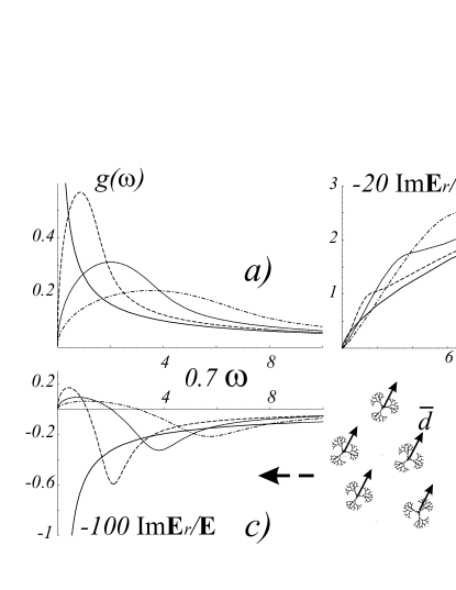
Figure 6: Density of states (a), optical response of surfaces covered by isolated fractals (b) and, merging fractals (c) when the inter-fractal distance is smaller compared to the fractal size. For a regular fractal (solid lines) one sees the power law dependencies corresponding to the fractal dimension $\alpha=1.41$ chosen. No typical energy reference exists for the unperturbed fractals, whereas for disordered fractals the typical energy is given by the disorder parameter $W=g_{O}<V^{2}>$ which is small (dashed line) medium (dotted line) or large (dash-dot line) with respect to the energy unit chosen.

The dependencies Eq.(34) are shown in Fig.6 for different sizes of the disorder parameter in the regime of both isolated and merging fractals. The power law dependence corresponding to the ideally symmetric fractals manifests itself as an asymptotic dependence for the irregularly perturbed fractals when the frequency exceeds the typical size of the parameter $W$ governing the disorder.

VI Acknowledgments

The authors express their gratitude to D.Khmelnitskii, V.Kravtsov, I.Procaccia and C.Textier for the discussions and for indication to relevant publications. One of the authors (V.A) also thanks Ph. Cahuzac and R.Larciprete for the discussion of the experimental feasibility of ellipsometric and internal reflection measurements.

References

- (1) L. Bardotti, P. Jensen, A. Hoareau, M. Treilleux, and B. Cabaud, Phys. Rev. Lett., 74, 4694 (1995)
- (2) C. Bréchignac, Ph. Cahuzac, F. Carlier, C. Colliex, M. de Frutos, N. Kébaili, J. Le Roux, A. Masson, and B. Yoon, Eur. Phys. J. D, 16, 265 (2001)
- (3) E. Borsella, M.A. Garcia, G.Mattei, C.Maurizio, P.Mazzoldi, E.Catturuzza, F.Gonella, G.Battaglin, A. Quaranta, and F.Dacapito, J. of Ap. Phys., 90, 4467 (2001)
- (4) S. Pratontep, P. Preece, C. Xirouchaki, R. E. Palmer, C. F. Sanz-Navarro, S. D. Kenny, and R. Smith, Phys Rev. Lett., 90, 055503 (2003)
- (5) V.M. Shalaev, R. Botet, D.P. Tsai, M. Moskovits, W.L. Mochan, R.G. Barrera, Physica-A, 207, 197 (1994)
- (6) V.A. Markel, L.S. Muratov, M.I. Stockman and T.F. George, Phys. Rev. B 43, 8183 (1991)
- (7) for a review see V.M. Shalaev, Phys. Rep., 272, 61 (1996)
- (8) Diffusive behavior corresponds both to the classical conductivity of metallic microfractals and to the multifractal structures of the energy eigen functions near the percolation limit associated with the metal-dielectric transition in the disordered metals, see D. E. Khmelnitskii, JETP Lett. 32 , 229, (1980); A. D. Mirlin and F. Evers Phys. Rev. B 62 , 7920 (2000). It also yields specific optical properties at low frequencies, see U. Sivan and Y. Imry, Phys. Rev. B 35, 6074 (1986)
- (9) E. I. Levin, M. E. Raikh, B. I. Shklovskii, Phys. Rev. B 44 , 11281 (1991)
- (10) B. Derrida and G.J. Rodgers, J. Phys. A, 26, L457, (1993)
- (11) A. D. Mirlin, and Y. V. Fyodorov, Phys. Rev. B 56, 13393 (1997)
- (12) B. L. Altshuler, Y. Gefen, A. Kamenev, L. S. Levitov, Phys. Rev. Lett.,78, 2803 (1997)
- (13) see e.g. K.G. Wilson, Phys. Rev. B 4, 3174 (1971); K.G. Wilson, Phys. Rev. B 4, 3184 (1971)
- (14) S. Blacher, F. Brouers, A. Sarychev, A. Ramsamugh and P. Gadenne, Langmuir, 12, 183 (1996)
- (15) V.I. Bukhtiyarov, A.F. Carley, L.A. Dollard and, M.W. Roberts, Surf. Sci., 381, L605 (1997)
- (16) P. Marquardt, Appl. Phys. A, 68, 211 (1999)
- (17) J.M. Barbaroux, J.M. Combes and R. Montcho, J. Math. Annal. and Appl., 213, 698 (1999)
- (18) V.M. Akulin, Phys. Rev. A48, 3532 (1993)
- (19) see e.g. A.A. Abrikosov, L.P. Gorkov, and I.E. Dzyaloshinski, Methods of quantum field theory in statistical physics, Dover Pub., N.Y. USA (1963);
- (20) K. Efetov, Supersymmetry in disorder and chaos, Cambridge Univ. Press, (1999)
- (21) C. Texier and, G. Montambaux, J. Phys. A 30, 10307 (2001)
- (22) see for instance J.W. Harris and,H. Stocker, Handbook of Mathematics and Computational Science, N.Y. Springer-Verlag, (1998)
- (23) L.A. Pastur, Theor. Math. Phys. (USSR), 10, 67, (1972)
- (24) E.M. Lifchitz, L.P. Pitaevskii Physical Kinetics §78
- (25) A.M. Dykhne, Sov. JETP, 32, 63 (1971)