On Quantum Bosonic Solids and Bosonic Superfluids

Abstract

We review the nature of superfluid ground states and the universality of their properties with emphasis to Bose Einstein Condensate systems in atomic physics. We then study the superfluid Mott transition in such systems. We find that there could be two types of Mott transitions and phases. One of them was described long ago and corresponds to suppression of Josephson tunneling within superfluids sitting at each well. On the other hand, the conditions of optical lattice BEC experiments are such that either the coherence length is longer than the interwell separation, or there is too small a number of bosons per well. This vitiates the existence of a superfluid order parameter within a well, and therefore of Josephson tunneling between wells. Under such conditions, there is a transition to a Mott phase which corresponds to suppression of individual boson tunneling among wells. This last transition is in general discontinuous and can happen for incommensurate values of bosons per site. If the coherence length is small enough and the number of bosons per site large enough, the transition studied in the earlier work will happen.

I Introduction

We have recently found us that bosonic systems in optical lattices can have discontinuous transitions from a superfluid phase to a Mott insulating phase irrespective of commensurability of the number of bosons and the number of lattice sites. This is contrary to expectations from the early theoretical work fisher . The discrepancy is not due to incorrectness in the early work, but due to that, depending on the physical conditions, the nature of the transition and the insulating phase can be different. Specifically for a small number of bosons per site and/or for superfluids with coherence length larger than the well size, the transition studied in the early work is impossible us2 , as it presupposes a superfluid order parameter within each well.

The nature of the Mott phase of the early work fisher is that of wells of superfluid, where the large repulsion prevents Josephson tunneling much as it happens in Josephson junctions arrays when the charging energy becomes large. The nature of our phase corresponds to when localization of single atoms in the wells destroys the superfluid order parameter. Our transition is necessarily first order as the superfluid order parameter, and hence the superfluid response, jumps discontinuously at the transition. The reason our transition necessarily destroys the superfluid order parameter is that, since our transition happens when the coherence length is larger than the well size or the interwell separation, boson localization introduces a length scale, the lattice constant, which is smaller than the coherence length for our transition. This leads to an energy scale larger than the superfluid ordering scale.

A Mott phase transition has recently been observed experimentally ib but the nature of the transition and of the Mott phase were not determined from such experiments. On the other hand, recent experiments are consistent with a discontinuous transition irrespective of commensurability ari .

In the present article we present the details leading to the conclusions of our earlier work. We present for the first time the explicit calculations, and we expand on the nature of the physics that controls when our transition is expected to happen as opposed to the transition predicted in the early work fisher is expected to take place. Since issues of superfluid ordering and the different energy scales in Bose Einstein Condensates (BECs) are essential for a microscopic understanding we start the article with sections that review well known physics of BECs and superfluids and their different length scales. We then study the nature of tunneling in optical lattices to review old results of ours us2 on the nature of tunneling in lattices of bosonic systems. When Josephson tunneling is suppressed before superfluid correlations are destroyed, the well known transition fisher follows. When superfluid correlations are destroyed before Josephson tunneling is suppressed, the transition we recently discovered follows us . We then move on to estimate the properties of the Mott phase and the energetics of when the Mott phase wins over the superfluid phase leading to a localization transition.

II Simple Bosonic Fluid Systems

In the present section we will review for completeness well known results in BECs and superfluid bosonic systems. Most of this knowledge is due to studies of superfluid He⁴ pines which predates the experimental realization of artificially engineered BECs beca ; becb ; becc . These are superfluid systems as they posses a finite sound speed bec2 ; landau ; bog and suppressed long-wavelength scattering bec3 ; bec4 . The superfluid phase has off-diagonal order with breaking of gauge invariance phil , i.e. $U(1)$ phase invariance, characterized by a coherent ground state of Bogolyubov pairs bog .

Even though much of the material in this section is far from new, we included it in the article for completeness and perspective for the subsequent sections. We also hope to give a flavor and emphasize the ideas of macroscopic exactness that characterize stable quantum and thermodynamic phases of matter. While this perspective is not new, it is hard to tell if its importance is properly recognized in the BEC and atomic physics community. It is our wish to stress its importance.

II.1 Noninteracting Boson Gas

A gas of noninteracting bosons is described by the Hamiltonian

$$\mathcal{H}=\sum_{\vec{k}}\epsilon_{\vec{k}}a_{\vec{k}}^{\dagger}a_{\vec{k}}$$ (1)

where the operators $a_{\vec{k}}$ and $a_{\vec{k}}^{\dagger}$ follow the harmonic oscillator commutator relations

$$[a_{\vec{k}}^{\dagger},a_{\vec{k}^{\prime}}^{\dagger}]=[a_{\vec{k}},a_{\vec{k}^{\prime}}]=0\;;\quad[a_{\vec{k}},a_{\vec{k}^{\prime}}^{\dagger}]=\delta_{{\vec{k}},{\vec{k}^{\prime}}}$$ (2)

In the continuum limit, the sum becomes and integral and $\epsilon_{0}=0$. The dispersion relation is

$$\epsilon_{\vec{k}}=\frac{\hbar^{2}k^{2}}{2m}$$ (3)

While in the continuum limit $|{\vec{k}}_{min}=0|$, in a finite box of size L with periodic boundary conditions

$${\vec{k}}=\frac{n_{x}\pi}{L}\hat{x}+\frac{n_{y}\pi}{L}\hat{y}+\frac{n_{z}\pi}{L}\hat{z}$$ (4)

where $n_{x}$, $n_{y}$, and $n_{z}$ are integers different from 0. Thus in the box $|{\vec{k}}_{min}|=\frac{\pi\sqrt{3}}{L}$ and there is a gap that vanishes in the thermodynamic limit, that is, it vanishes as the number of bosons goes to infinity such that the density is fixed. For an optical lattice system the boson dispersion at long wavelengths is exactly as the one above for an appropriately chosen mass.

The ground state wavefunction is trivial.

$$|\Psi_{0}\rangle=a_{0}^{N}|0\rangle$$ (5)

where $a_{0}=a_{{\vec{k}}_{min}}$. This wavefunction reflects the fact that bosons can occupy the same state, so the ground state will consists of all N particles in the minimum energy state. This state has energy $\epsilon_{0}=0$ in the continuum limit. All the particles are coherent and have the “same phase”: Bose Einstein condensation has occurred. This is the preamble to the occurrence of the phenomenon of superfluidity. Bose condensation is a necessary condition for superfluidity to occur, but it is not a sufficient condition. Bose condensation implies that, when the continuum limit is an appropriate approximation, the system is a quantum fluid. As explained below, a noninteracting Bose condensate lacks the necessary rigidity of the ground state wavefunction. A rigid ground state wavefunction means that the dispersion relation is such that as ${\bf k}\rightarrow 0$, the excitation of quasiparticles costs an energy higher than $\frac{\hbar^{2}{\vec{k}}^{2}}{2m}$. Dissipation processes are prohibited when the system has enough rigidity as they would violate energy momentum conservation. Dissipationless response is the definition of superfluidity as the coherence of the condensate can then survive weak enough perturbations. This necessary rigidity is provided by repulsive interactions among the bosons comprising the superfluid. In the absence of such interactions, the lack of rigidity permits scattering processes to occur which degrade coherence no matter how weakly the system is perturbed.

II.2 Interacting Boson Gas

BECs are really systems of bosons with repulsive interactions among them. They are supersaturated quantum vapors because they are metastable. They behave like quantum mechanical ground states for some time, but due to interactions or trap effects they loose stability and decay. Since they live long enough to do measurements of their properties, and we can do calculations that agree with experiments as if they were ground states, it is not incorrect to treat them as ground states for times longer than their lifetimes. The finite lifetimes are both due to increasing interactions and trap effects. Usually their lifetimes are “long enough” that a lot of “ground state” physics can be studied. We concentrate in this latter physics.

We will look here at some of the properties of BECs. Another system that can be described in an exactly the same manner and is actually a ground state is superfluid He⁴. The fact that is a liquid is not contradictory since the elementary excitations of the liquid have to repel each other as a stability condition. Otherwise, the elementary excitations can condense leading to some other phase of matter.

We now proceed to describe the ground state and low energy excitation properties of the interacting Bose gas. We will concentrate on a boson system on a lattice with onsite Hubbard repulsion as we have bosons systems in optical lattices in mind. We do emphasize that the physics we describe here is universal as long as the system is a quantum fluid, i.e. there exists a macroscopically occupied lowest momentum state, and there is repulsion among the long wavelength elementary excitations of the system. When these two conditions are met, the physics is independent of the microscopic details of your system.

We now concentrate on the Bose Hubbard Hamiltonian in a lattice (which of course can be an optical lattice)

$$\mathcal{H}=\frac{-t}{2}\sum_{<ij>}(a_{i}^{\dagger}a_{j}+a_{j}^{\dagger}a_{i})-\mu\sum_{i}a_{i}^{\dagger}a_{i}\\ +U\sum_{i}a_{i}^{\dagger}a_{i}(a_{i}^{\dagger}a_{i}-1)-\varepsilon\sum_{i}a_{i}^{\dagger}a_{i}$$ (6)

where $\mu$ is a chemical potential, $U$ is the repulsion between bosons, $t$ is the tunneling amplitude between sites or hopping term, and $\varepsilon$ represents the depth of the potential well. In a Mott insulating phase with localized bosons $\mu$ is irrelevant and can be set equal to 0. It is needed to describe the superfluid phase, as the approximations made in the Bogolyubov Hamiltonian make the number of particles to not be conserved. In that case $\mu$ is chosen in such a way that the average number of particles equals the total number of particles in the system. In the thermodynamic limit, the fluctuations around the average number of particles become negligible compared to the average. We emphasize that the nonconservation of particles in the Bogolyubov approximation is an artifact of the approximation. Physically the total number of bosons in the system is, of course, constant, but the number of bosons in the condensate cannot be constant due to spontaneous breaking of phase invariancephil .

We consider a system with $M$ bosons and $N$ lattice sites. The number of bosons need not be commensurate with the lattice, i.e. $M/N$ need not be an integer. The Hubbard interaction term in the Hamiltonian is after Fourier transforming

$$\mathcal{H}_{I}=\frac{U}{N}\sum_{{\vec{q}},{\vec{k}}_{1},{\vec{k}}_{2}}\sum_{{\vec{k}}_{3},{\vec{k}}_{4}}a_{{\vec{k}}_{3}}^{\dagger}a_{{\vec{k}}_{1}}a_{{\vec{k}}_{4}}^{\dagger}a_{{\vec{k}}_{2}}\\ \times\delta({\vec{q}}+{\vec{k}}_{1}-{\vec{k}}_{3})\;\delta({\vec{k}}_{2}-{\vec{k}}_{4}-{\vec{q}})$$ (7)

Performing some momentum summations we get to

$$\mathcal{H}_{I}=\frac{U}{N}\sum_{{\vec{k}}_{1},{\vec{k}}_{2}}\sum_{\vec{q}}a_{{\vec{k}}_{1}+{\vec{q}}}^{\dagger}a_{{\vec{k}}_{1}}a_{{\vec{k}}_{2}-{\vec{q}}}^{\dagger}a_{{\vec{k}}_{2}}$$ (8)

The kinetic energy is a sum over pairs of nearest neighbors which describes tunneling from site to site:

$$\mathcal{H}_{K}=\frac{-t}{2}\sum_{\delta,i}(a_{i+\delta}^{\dagger}a_{i}+a_{i}^{\dagger}a_{i+\delta})=-t\sum_{\delta,i}a_{i+\delta}^{\dagger}a_{i}$$ (9)

where $\delta$ is one of the vectors from a particle to its nearest neighbor. Fourier transforming diagonalizes the kinetic energy giving

$$\mathcal{H}_{k} =-t\sum_{\delta,{\vec{k}}}e^{-i{\vec{k}}\cdot{\bf r}_{\delta}}a_{\vec{k}}^{\dagger}a_{\vec{k}}$$

$$=\sum_{\vec{k}}\epsilon_{\vec{k}}n_{\vec{k}}$$ (10)

where $\epsilon_{\vec{k}}$ is the dispersion

$$\epsilon_{\vec{k}}=-t\sum_{\delta}e^{-i{\vec{k}}\cdot{\bf r}_{\delta}}$$ (11)

for a cubic lattice, with the energy measured from the state of zero momentum

$$\epsilon_{\vec{k}}=-2t(\cos{k_{x}a}+\cos{k_{y}a}+\cos{k_{z}a})+6t$$ (12)

This shift of the zero of energy is irrelevant to the physics as it can be absorbed in a redefinition of the chemical potential. The dispersion goes like $ta^{2}k^{2}=\hbar^{2}k^{2}/2m$ in the long wavelength limit. We see that efficient tunneling corresponds to light particles and suppressed tunneling to very heavy ones. The full interacting boson Hamiltonian is then

$$\mathcal{H}=\frac{U}{N}\sum_{{\vec{k}}_{1},{\vec{k}}_{2}}\sum_{\vec{q}}a_{{\vec{k}}_{1}+{\vec{q}}}^{\dagger}a_{{\vec{k}}_{1}}a_{{\vec{k}}_{2}-{\vec{q}}}^{\dagger}a_{{\vec{k}}_{2}}\\ +\sum_{\vec{k}}\epsilon_{\vec{k}}a_{\vec{k}}^{\dagger}a_{\vec{k}}-(\mu+\varepsilon+U)\sum_{\vec{k}}a_{\vec{k}}^{\dagger}a_{\vec{k}}\\ -6t\sum_{\vec{k}}a_{\vec{k}}^{\dagger}a_{\vec{k}}\qquad\qquad\qquad\qquad$$ (13)

Now that we have ended with the Bose Hubbard Hamiltonian, we will consider ground state and low energy excitation properties. At low temperatures a macroscopic number of bosons occupy the zero momentum state as long as $U$ is not too high. This is what it means to be Bose condensed. We take the number of bosons in the condensate to be $M_{0}$. A quantum state with a large quantum number behaves classically. An operator acting on that state corresponding to the large quantum number can be treated as a $c-$number, for its fluctuations are negligible and its quantum behavior is not seen. It is then possible to replace $a_{0}$ and $a_{0}^{\dagger}$ by $\sqrt{M_{0}}$, the square root of the total number of bosons in the condensate. For completeness we review all the tedious algebraic manipulations leading to the reduced Bogolyubov Hamiltonianbog ; pines in appendix A:

$$\mathcal{H}=\frac{M_{0}^{2}}{N}U+\sum_{{\vec{k}}\neq 0}\tilde{\epsilon}_{\vec{k}}\;a_{\vec{k}}^{\dagger}a_{\vec{k}}+\frac{M_{0}U}{N}\sum_{{\vec{k}}\neq 0}(a_{\vec{k}}^{\dagger}a_{-{\vec{k}}}^{\dagger}+a_{-{\vec{k}}}a_{\vec{k}})$$ (14)

where $\tilde{\epsilon}_{\vec{k}}=\epsilon_{\vec{k}}+4M_{0}U/N-\mu$ and $\varepsilon$ and $U$ factors have been subsumed in $\mu$ as the fixing of the average particle number will cause them to be swallowed by the chemical potential.

For the ground state, which is a minimum of energy, the expectation value of $\mathcal{H}$ must satisfy

$$\frac{\partial\langle\mathcal{H}\rangle}{\partial M_{0}}=0$$

If this condition is not satisfied, then by connecting a reservoir to our system we would have a flow of particles into and out of the system until equilibrium is reached. As long as the low energy eigenstates do not deplete the condensate, which they do not for not too high $U$, they satisfy the same extremum condition. Taking the partial derivative we find

$$\mu=\frac{2M_{0}}{N}U$$ (15)

and

$$\tilde{\epsilon}_{\vec{k}}=\epsilon_{\vec{k}}+\frac{2M_{0}}{N}U$$ (16)

The Hamiltonian in equation (14) can be diagonalized by making a Bogolyubov transformation

$$b_{\vec{k}}=u_{\vec{k}}a_{\vec{k}}+v_{\vec{k}}a_{-{\vec{k}}}^{\dagger}\qquad b_{\vec{k}}^{\dagger}=u_{\vec{k}}a_{\vec{k}}^{\dagger}+v_{\vec{k}}a_{-{\vec{k}}}$$ (17)

where we require

$$[b_{\vec{k}},b_{\vec{k}}^{\dagger}]=u_{\vec{k}}^{2}-v_{\vec{k}}^{2}=1$$ (18)

in order for the transformation to be canonical. The diagonal Hamiltonian has the form

$$\mathcal{H}=\sum_{\vec{k}}E_{\vec{k}}b_{\vec{k}}^{\dagger}b_{\vec{k}}+C$$

where $C$ is a constant. Substituting (17) in the above expression we find

$$\mathcal{H}=\sum_{\vec{k}}(E_{\vec{k}}\;(u_{\vec{k}}^{2}+v_{\vec{k}}^{2})\;a_{\vec{k}}^{\dagger}a_{\vec{k}}+u_{\vec{k}}v_{\vec{k}}E_{\vec{k}}(a_{\vec{k}}^{\dagger}a_{-{\vec{k}}}^{\dagger}+a_{-{\vec{k}}}a_{\vec{k}})\\ +E_{\vec{k}}v_{\vec{k}}^{2})+C$$ (19)

Comparing this expression with (14) we identify

$$E_{\vec{k}}\;(u_{\vec{k}}^{2}+v_{\vec{k}}^{2})=\tilde{\epsilon}_{\vec{k}}\qquad u_{\vec{k}}v_{\vec{k}}E_{\vec{k}}=\frac{M_{0}}{N}U$$

Solving these two equations together with $u_{\vec{k}}^{2}-v_{\vec{k}}^{2}=1$ yields

$$u_{\vec{k}}=\frac{1}{\sqrt{2}}\sqrt{\frac{\tilde{\epsilon}_{\vec{k}}}{E_{\vec{k}}}+1}\qquad v_{\vec{k}}=\frac{1}{\sqrt{2}}\sqrt{\frac{\tilde{\epsilon}_{\vec{k}}}{E_{\vec{k}}}-1}$$ (20)

$$E_{\vec{k}}^{2} =\tilde{\epsilon}_{\vec{k}}^{2}-\frac{4M_{0}^{2}}{N^{2}}U^{2}$$

$$E_{\vec{k}} =\sqrt{\epsilon_{\vec{k}}}\sqrt{\epsilon_{\vec{k}}+4\frac{M_{0}}{N}U}$$ (21)

This is the quasiparticle excitation spectrum. As $k\rightarrow 0$

$$E_{\vec{k}}\simeq\sqrt{\epsilon_{\vec{k}}}\sqrt{\frac{4M_{0}U}{N}}=p\sqrt{\frac{2M_{0}U}{Nm}}$$ (22)

where $p=\sqrt{2m\epsilon_{\vec{k}}}=\sqrt{2mt}\;ak=\hbar k$. Since as $k\rightarrow 0$, $E_{\vec{k}}=pc_{s}$, i.e. low energy excitations are sound, we identify the speed of sound to be

$$c_{s}=\sqrt{\frac{2M_{0}U}{Nm}}$$ (23)

This is a finite measurable quantity that indicates the presence of correlations among the constituents of the material. Such correlations stabilize persistent currents and give rigidity to the ground state by making it energetically expensive to excite the fundamental bosons independently. Instead, the excitations are collective modes and the system superflows. The ground state has acquired rigidity. Artificially engineered BECs have been measured to have finite sound speedsbec2 and are thus superfluid.

The ground state wavefunction is worked out appendix B and found to be

$$\qquad\quad|\Psi_{0}\rangle=\prod_{\vec{k}}\frac{1}{u_{\vec{k}}}e^{-(v_{\vec{k}}/u_{\vec{k}})a_{\vec{k}}^{\dagger}a_{-\vec{k}}^{\dagger}}\;(a_{0}^{\dagger})^{M_{0}}|0\rangle$$ (24)

The factor $(a_{0}^{\dagger})^{M_{0}}$ represents the bosons in the condensate. In the absence of interactions, $u_{\vec{k}}=1,v_{\vec{k}}=0$, so that in exciting bosons, one changes atomic boson number by one. In the presence of interactions, states with momentum ${\vec{k}}$ and $-{\vec{k}}$ are mixed into the ground state, so when an excitation with momentum ${\vec{k}}$ is created, another with momentum $-{\vec{k}}$ is destroyed. The excitations are coherent superpositions of atoms and “holes”. This is due to the nature of the coupling between ${\vec{k}}$ and $-{\vec{k}}$ in the Bogolyubov operators. With interactions both $u_{\vec{k}}$ and $v_{\vec{k}}$ increase.

The ground state contains nonseparable, nontrivial correlations between the bosons that make up the system, i. e., it is entangled. The correlations in the ground state have entangled the bosons into a coherent state for the lowest energy state. The entanglement is so extreme that the bosons that make up the system cannot be excited at long wavenumbers. Their existence at low energies is impossible. Only sound can be excited, i.e. the excitations are Bogolyubov quasiparticles which do not resemble bosons whatsoever at low energies. In this limit, the principles of quantum hydrodynamics become exact because the system does not dissipate and sound excitations become exact eigenstates of the system. The boson fluid responds only collectively at long wavelengths. Aspects of the universality of superfluid physics are presented in appendix C

We now proceed to calculate the self-consistency condition. Using the ground state wave function (24) the self-consistency condition is

$$\sum_{i}\langle n_{i}\rangle=M=\langle\Psi_{0}|a_{0}^{\dagger}a_{0}|\Psi_{0}\rangle+\sum_{\vec{k}\neq 0}\langle\Psi_{0}|a_{\vec{k}}^{\dagger}a_{\vec{k}}|\Psi_{0}\rangle$$ (25)

Let $|a\rangle=a_{\vec{k}}|\Psi_{0}\rangle$, that is

$$|a\rangle=\prod_{{\vec{k}}^{\prime}\neq{\vec{k}}}\frac{1}{u_{{\vec{k}}^{\prime}}}e^{-\frac{v_{{\vec{k}}^{\prime}}}{u_{{\vec{k}}^{\prime}}}a_{{\vec{k}}^{\prime}}^{\dagger}a_{-{\vec{k}}^{\prime}}^{\dagger}}\frac{1}{u_{\vec{k}}}e^{-\frac{v_{\vec{k}}}{u_{\vec{k}}}a_{\vec{k}}^{\dagger}a_{-{\vec{k}}}^{\dagger}}|0\rangle$$ (26)

The commutation relation $[a_{\vec{k}},a_{\vec{k}}^{\dagger}]=1$ implies $a_{\vec{k}}=\frac{\partial}{\partial a_{\bf k}^{\dagger}}$. Using this result

$$|a\rangle=-\frac{v_{\vec{k}}}{u_{\vec{k}}}a_{-{\vec{k}}}^{\dagger}|\Psi_{0}\rangle$$ (27)

Substituting the Bogolyubov transformation $a_{-{\vec{k}}}^{\dagger}=u_{\vec{k}}b_{-{\vec{k}}}^{\dagger}-v_{\vec{k}}b_{\vec{k}}$

$$|a\rangle=-\frac{v_{\vec{k}}}{u_{\vec{k}}}(u_{\vec{k}}b_{-{\vec{k}}}^{\dagger}-v_{\vec{k}}b_{\vec{k}})|\Psi_{0}\rangle=-v_{\vec{k}}b_{-{\vec{k}}}^{\dagger}|\Psi_{0}\rangle$$ (28)

Thus $\langle a|a\rangle=v_{\vec{k}}^{2}$ and the self-consistency condition becomes

$$M =\sum_{\vec{k}}v_{\vec{k}}^{2}+M_{0}=\frac{1}{2}\sum_{\vec{k}}\frac{\tilde{\epsilon}_{\vec{k}}-E_{\vec{k}}}{E_{\vec{k}}}+M_{0}$$

$$=\frac{1}{2}\sum_{\vec{k}}\left(\frac{\epsilon_{\vec{k}}+2(M_{0}/N)U}{E_{\vec{k}}}-1\right)+M_{0}$$ (29)

This is the “particle conservation sum rule”.

We will now make estimates of the number of particles in the condensate as a function of $U/t$. We use the result (II.2)

$$v_{\vec{k}}^{2}=\frac{1}{2}\left(\frac{\epsilon_{\vec{k}}+2(M_{0}/N)U}{\sqrt{\epsilon_{k}}\sqrt{\epsilon_{\vec{k}}+4(M_{0}/N)U}}-1\right)$$ (30)

Similarly we will also estimate

$$u_{\vec{k}}^{2}=\frac{1}{2}\left(\frac{\epsilon_{\vec{k}}+2(M_{0}/N)U}{\sqrt{\epsilon_{k}}\sqrt{\epsilon_{\vec{k}}+4(M_{0}/N)U}}+1\right)$$ (31)

We will concentrate on the long wavelength behavior, where equation (12) for the dispersion gives $\epsilon_{\vec{k}}\simeq tk^{2}a^{2}$. In this limit, the sum over ${\vec{k}}$ will be approximated with an integral: $\sum_{\vec{k}}\rightarrow(Na^{3}/2^{3}\pi^{3})\int k^{2}\;dk\;d\Omega$. Here $N$ is the number of lattice sites. Notice further that for $\epsilon_{\vec{k}}\simeq tk^{2}a^{2}<2UM_{0}/N$, $v_{\vec{k}}\neq 0$ and $u_{\vec{k}}\neq 1$. On the other hand, for $tk^{2}a^{2}>>2UM_{0}/N$, $v_{\vec{k}}\simeq 0$ and $u_{\vec{k}}\simeq 1$. This means that the system behaves like a superfluid for long wavelengths and like a free Bose gas for short wavelengths. Superfluidity is thus a low energy phenomenon. This behavior can be approximated with the introduction of a cutoff, so that above the cutoff $v_{\vec{k}}\simeq 0$ and $u_{\vec{k}}\simeq 1$ while below the cutoff they are given by the integral through the region $0\leq k\leq k_{c}$. The cutoff is given by

$$tk_{c}^{2}a^{2}=2\frac{UM_{0}}{N}\qquad;\qquad k_{c}=\frac{\sqrt{2}}{a}\sqrt{\frac{UM_{0}}{tN}}$$ (32)

For $k<k_{c}$ the system responds like a superfluid while otherwise it behaves like a dissipative free Bose gas. The important detail is that as long as the cutoff wavevector is smaller than the absolute cutoff from the lattice, $\pi/a$, so that $\frac{2UM_{0}}{tN\pi^{2}}\leq 1$, it will define the cutoff for all momentum integrals is $k_{c}$. The system generated a cutoff scale from the physics that lead to superfluidity. This scale is related to the all important coherence length of the superfluid about which we will have a lot to say later. Going back to (30) and writing $\epsilon_{{\vec{k}}_{c}}$ for $2UM_{0}/N$

$$v_{\vec{k}}^{2} =\frac{1}{2}\left(\frac{\epsilon_{\vec{k}}+\epsilon_{{\vec{k}}_{c}}}{\sqrt{\epsilon_{k}}\sqrt{\epsilon_{\vec{k}}+2\epsilon_{{\vec{k}}_{c}}}}-1\right)$$

$$\simeq\frac{1}{2}\left(\frac{1}{\sqrt{2}}\sqrt{\frac{\epsilon_{{\vec{k}}_{c}}}{\epsilon_{\vec{k}}}}-1\right)$$ (33)

and

$$u_{\vec{k}}^{2}\simeq\frac{1}{2}\left(\frac{1}{\sqrt{2}}\sqrt{\frac{\epsilon_{{\vec{k}}_{c}}}{\epsilon_{\vec{k}}}}+1\right)$$ (34)

In terms of the cutoff

$$v_{\vec{k}}^{2}\simeq\frac{1}{2}\left(\frac{1}{\sqrt{2}}\frac{k_{c}}{k}\right)\simeq u_{\vec{k}}^{2}$$ (35)

Thus

$$\sum_{\vec{k}}v_{\vec{k}}^{2}\simeq\frac{Na^{3}k_{c}}{16\sqrt{2}\pi^{3}}\int_{0}^{k_{c}}\frac{1}{k}\;d^{3}{\vec{k}}=\frac{1}{8\sqrt{2}\pi^{2}}Na^{3}k_{c}^{3}$$ (36)

Substituting this into (II.2) gives for the self-consistency condition

$$M=\frac{1}{8\sqrt{2}\pi^{2}}Na^{3}k_{c}^{3}+M_{0}$$ (37)

This provides an expression for $U/t$ in terms of $M_{0}/M$:

$$1 =\frac{1}{8\sqrt{2}\pi^{2}}a^{3}k_{c}^{3}\frac{N}{M}+\frac{M_{0}}{M}$$

$$1 =\frac{1}{8\sqrt{2}\pi^{2}}\left(\frac{2M_{0}U}{Nt}\right)^{3/2}\frac{N}{M}+\frac{M_{0}}{M}$$

$$\frac{U}{t} =(8\sqrt{2}\pi^{2})^{2/3}\frac{N}{2M_{0}}\left(\frac{M}{N}\right)^{2/3}\left(1-\frac{M_{0}}{M}\right)^{2/3}$$ (38)

We now proceed to calculate the expected value of the Bose Hubbard Hamiltonian in the superfluid ground state in order to compare with the energy of the other phases and see which one is energetically more favorable. One of the main concerns of the present work is the Mott transition. So in particular we will compare this ground state energy of the superfluid phase with a certain Mott phase not previously studied in the literaturefisher . The full Bose Hubbard Hamiltonian is given in equation (13). The expectation value of the energy in the superfluid ground state is then

$$\langle\mathcal{H}\rangle=-(\varepsilon+U)M+\sum_{\vec{k}}\epsilon_{\vec{k}}v_{\vec{k}}^{2}\\ +\frac{U}{N}\sum_{{\vec{k}}_{1},{\vec{k}}_{2}}\sum_{\vec{q}}\langle a_{{\vec{k}}_{1}+{\vec{q}}}^{\dagger}a_{{\vec{k}}_{1}}a_{{\vec{k}}_{2}-{\vec{q}}}^{\dagger}a_{{\vec{k}}_{2}}\rangle-6tM$$ (39)

Notice that $a_{{\vec{k}}_{1}}a_{{\vec{k}}_{2}-{\vec{q}}}=\delta_{{\vec{k}}_{1},{\vec{k}}_{2}-{\vec{q}}}+a_{{\vec{k}}_{2}-{\vec{q}}}^{\dagger}a_{{\vec{k}}_{1}}$. Using this result we obtain for the interaction term

$$\langle\mathcal{H}_{I}\rangle =\frac{U}{N}\sum_{{\vec{k}}_{2},{\vec{q}}}a_{{\vec{k}}_{2}}^{\dagger}a_{{\vec{k}}_{2}}+\frac{U}{N}\sum_{{\vec{k}}_{1},{\vec{k}}_{2}}\sum_{\vec{q}}\langle a_{{\vec{k}}_{1}+{\vec{q}}}^{\dagger}a_{{\vec{k}}_{2}-{\vec{q}}}^{\dagger}a_{{\vec{k}}_{1}}a_{{\vec{k}}_{2}}\rangle$$

$$=UM+\frac{U}{N}\sum_{{\vec{k}}_{1},{\vec{k}}_{2}}\sum_{\vec{q}}\langle a_{{\vec{k}}_{1}+{\vec{q}}}^{\dagger}a_{{\vec{k}}_{2}-{\vec{q}}}^{\dagger}a_{{\vec{k}}_{1}}a_{{\vec{k}}_{2}}\rangle$$ (40)

On the other hand we have from (D)

$$a_{{\vec{k}}_{1}}a_{{\vec{k}}_{2}}|\Psi_{0}\rangle =\frac{-v_{{\vec{k}}_{2}}}{u_{{\vec{k}}_{2}}}(1+\frac{v_{{\vec{k}}_{1}}^{2}u_{{\vec{k}}_{2}}}{u_{{\vec{k}}_{1}}})\delta_{{\vec{k}}_{1},-{\vec{k}}_{2}}|\Psi_{0}\rangle$$

$$\qquad\qquad+v_{{\vec{k}}_{1}}v_{{\vec{k}}_{2}}b_{-{\vec{k}}_{1}}^{\dagger}b_{-{\vec{k}}_{2}}^{\dagger}|\Psi_{0}\rangle$$

Similarly

$$\langle\Psi_{0}|a_{{\vec{k}}_{1}+{\vec{q}}}^{\dagger}a_{{\vec{k}}_{2}-{\vec{q}}}^{\dagger} =\frac{-v_{{\vec{k}}_{1}+{\vec{q}}}}{u_{{\vec{k}}_{1}+{\vec{q}}}}(1+\frac{v_{{\vec{k}}_{2}-{\vec{q}}}^{2}u_{{\vec{k}}_{1}+{\vec{q}}}}{u_{{\vec{k}}_{2}-{\vec{q}}}})\langle\Psi_{0}|\;\delta_{{\vec{k}}_{1},-{\vec{k}}_{2}}$$

$$+v_{{\vec{k}}_{2}-{\vec{q}}}v_{{\vec{k}}_{1}+{\vec{q}}}\langle\Psi_{0}|\;b_{-{\vec{k}}_{1}-{\vec{q}}}b_{-{\vec{k}}_{2}+{\vec{q}}}$$

Joining the two results we finally get

$$\langle a_{{\vec{k}}_{1}+{\vec{q}}}^{\dagger}a_{{\vec{k}}_{2}-{\vec{q}}}^{\dagger}a_{{\vec{k}}_{1}}a_{{\vec{k}}_{2}}\rangle =\frac{v_{{\vec{k}}_{2}}}{u_{{\vec{k}}_{2}}}\frac{v_{{\vec{k}}_{1}+{\vec{q}}}}{u_{{\vec{k}}_{1}+{\vec{q}}}}(1+\frac{v_{{\vec{k}}_{1}}^{2}u_{{\vec{k}}_{2}}}{u_{{\vec{k}}_{1}}})(1+\frac{v_{{\vec{k}}_{2}-{\vec{q}}}^{2}u_{{\vec{k}}_{1}+{\vec{q}}}}{u_{{\vec{k}}_{2}-{\vec{q}}}})\delta_{{\vec{k}}_{1},-{\vec{k}}_{2}}+v_{{\vec{k}}_{1}}v_{{\vec{k}}_{2}}v_{{\vec{k}}_{2}-{\vec{q}}}v_{{\vec{k}}_{1}+{\vec{q}}}\langle b_{-{\vec{k}}_{1}-{\vec{q}}}b_{-{\vec{k}}_{2}+{\vec{q}}}b_{-{\vec{k}}_{1}}^{\dagger}b_{-{\vec{k}}_{2}}^{\dagger}\rangle$$

$$=\frac{v_{{\vec{k}}_{2}}}{u_{{\vec{k}}_{2}}}\frac{v_{{\vec{k}}_{1}+{\vec{q}}}}{u_{{\vec{k}}_{1}+{\vec{q}}}}(1+\frac{v_{{\vec{k}}_{1}}^{2}u_{{\vec{k}}_{2}}}{u_{{\vec{k}}_{1}}})(1+\frac{v_{{\vec{k}}_{2}-{\vec{q}}}^{2}u_{{\vec{k}}_{1}+{\vec{q}}}}{u_{{\vec{k}}_{2}-{\vec{q}}}})\delta_{{\vec{k}}_{1},-{\vec{k}}_{2}}$$

$$\qquad\qquad\qquad+v_{{\vec{k}}_{1}}v_{{\vec{k}}_{2}}v_{{\vec{k}}_{2}-{\vec{q}}}v_{{\vec{k}}_{1}+{\vec{q}}}(\delta_{-{\vec{k}}_{2}+{\vec{q}},-{\vec{k}}_{1}}\delta_{-{\vec{k}}_{1}-{\vec{q}},-{\vec{k}}_{2}}+\delta_{-{\vec{k}}_{2}+{\vec{q}},-{\vec{k}}_{2}}\delta_{-{{\vec{k}}_{1}}-{\vec{q}},-{\vec{k}}_{1}})$$ (41)

Thus performing the sums

$$\sum_{{\vec{k}}_{1},{\vec{k}}_{2}}\sum_{\vec{q}}\langle a_{{\vec{k}}_{1}+{\vec{q}}}^{\dagger} a_{{\vec{k}}_{2}-{\vec{q}}}^{\dagger}a_{{\vec{k}}_{1}}a_{{\vec{k}}_{2}}\rangle\qquad\qquad\qquad\qquad\qquad\qquad$$

$$=\sum_{{\vec{k}},{\vec{k}}_{1}}\frac{v_{\vec{k}}}{u_{\vec{k}}}\frac{v_{{\vec{k}}_{1}}}{u_{{\vec{k}}_{1}}}(1+v_{\vec{k}}^{2})(1+v_{{\vec{k}}_{1}}^{2})$$

$$\qquad\qquad+2\sum_{{\vec{k}},{\vec{k}}^{\prime}}v_{\vec{k}}^{2}v_{{\vec{k}}^{\prime}}^{2}$$ (42)

where ${\vec{k}}_{1}\equiv{\vec{k}}-{\vec{q}}$. From (33) and (34) $u_{\vec{k}}^{2}/v_{\vec{k}}^{2}=1$. Hence

$$\sum_{\vec{k}}\frac{v_{\vec{k}}}{u_{\vec{k}}}\simeq\frac{Na^{3}}{2^{3}\pi^{3}}\int_{0}^{k_{c}}\;d^{3}{\vec{k}}=\frac{1}{6\pi^{2}}Na^{3}k_{c}^{3}$$ (43)

Usage of (36) and (43) into (II.2) gives

$$\sum_{{\vec{k}}_{1},{\vec{k}}_{2}}\sum_{\vec{q}}\langle a_{{\vec{k}}_{1}+{\vec{q}}}^{\dagger}a_{{\vec{k}}_{2}-{\vec{q}}}^{\dagger}a_{{\vec{k}}_{1}}a_{{\vec{k}}_{2}}\rangle$$

$$\simeq\left(\frac{1}{9}+\frac{1}{6\sqrt{2}}+\frac{1}{32}\right)\frac{N^{2}a^{6}k_{c}^{6}}{4\pi^{4}}$$ (44)

As for the kinetic energy, with $\epsilon_{\vec{k}}\simeq tk^{2}a^{2}$ and (33)

$$\sum_{\vec{k}}\epsilon_{\vec{k}}v_{\vec{k}}^{2} \simeq\frac{Na^{3}}{16\sqrt{2}\pi^{3}}ta^{2}k_{c}\int_{0}^{k_{c}}k\;d^{3}{\vec{k}}$$

$$=\frac{1}{16\sqrt{2}\pi^{2}}Nta^{5}k_{c}^{5}$$ (45)

Substituting (II.2), (II.2) and (II.2) into (39) gives

$$\langle\mathcal{H}\rangle\simeq -\varepsilon M+\frac{1}{16\sqrt{2}\pi^{2}}Nta^{5}k_{c}^{5}$$

$$+NU\left(\frac{1}{9}+\frac{1}{6\sqrt{2}}+\frac{1}{32}\right)\frac{a^{6}k_{c}^{6}}{4\pi^{4}}$$

$$-6tM$$

$$= -\varepsilon M+\frac{1}{16\sqrt{2}\pi^{2}}Nt\left(\frac{2M_{0}U}{Nt}\right)^{5/2}$$

$$+\left(\frac{1}{9}+\frac{1}{6\sqrt{2}}+\frac{1}{32}\right)\frac{NU}{4\pi^{4}}\left(\frac{2M_{0}U}{Nt}\right)^{3}$$

$$-6tM$$ (46)

If the number of bosons is an integer multiple of the number of lattice sites, the system is said to be commensurate. On the other hand, if the number of bosons is not an integer multiple of the number of lattice sites, the system is said to be incommensurate. Notice that the above result is general and thus applies for both incommensurate and commensurate systems.

In the limit of small $U/t$, $M_{0}\simeq M$ and the second and third terms are small. The energetically expensive term, $UN$ is small. There is an energy gain in becoming superfluid. As $U/t$ increases $\frac{UM_{0}}{tN}$ goes to a constant as we will see in a succeeding section, and the second and third become of the order of $N$. If the second and third terms cancel the kinetic energy term $-6tM$, the system is not a quantum fluid anymore. It will thus have a transition into an insulating phase, a Mott phase. The commensurability does not play a role in the depletion of the condensate, contrary to what was found in the earlier work fisher . The earlier work is not incorrect. In that work, the Mott transition happens when the superfluid within each well dephases, preventing Josephson tunneling and leading to a Mott-phase. That transition is continuous and only possible for commensurate values. For this to happen there needs to exist a superfluid within each well, which requires enough bosons per well (broken symmetries can only happen for a macroscopic number of particles) and the coherence length to be longer than the well. So in certain physical situations there is a Mott transition of a different type, discontinuous and incommensurate, since the superfluid does not survive within each well, and individual bosons are localized in each well. We will elucidate these physics in following sections.

III Order Parameter in the Superfluid

In the present section we go on with the study of the universal properties of the superfluid. We concentrate in what is the superfluid order parameter. This section also provides a connection with the new kind of Mott transition we have uncovered in our work. In particular, since we will find that the superfluid order parameter increases as we increase the onsite repulsion $U$, i.e. as we approach a Mott transition, a transition in which the superfluid order parameter is destroyed must be discontinuous. The unique experimental signature of this is a discontinuous jump in any measure of the superfluid response.

We have seen that the well depth $\varepsilon$ is subsumed into the chemical potential upon minimization of the ground state energy with respect to the number of particles in the condensate. The physical reason for this is that whether the lattice is deep or shallow is irrelevant as long as the system is superfluid; it superflows through it. Nonetheless, the well depth is relevant to the Mott transitions and phases. Also, the kinetic term in (6) depends on $\varepsilon$. This is so because decreasing the depth of the potential well, i.e. increasing $\varepsilon$, will obviously decrease $t$ as the barrier through which tunneling must occur is higher. The only vestige of $\varepsilon$ remaining in the superfluid is through $t(\varepsilon)$. We also notice that $U/t\rightarrow\infty$ with decreasing $t$. This however does not kill the order parameter of the BEC as long as the condensate is not depleted or Josephson tunneling suppressed. If the condensate is depleted there will be a Mott transition in the universality class of the one uncovered in the present work. If Josephson tunneling is suppressed without destruction of the order parameter, there will be a Mott transition in the universality class discovered in the previous class fisher .

It is commonly said in the literature that the existence of a condensate is essential for superfluidity. The macroscopic occupation of the lowest momentum state, i.e. the presence of the condensate, makes the boson system into a quantum fluid as long as the separation between energy levels is unmeasurable. The existence of the condensate does not imply the existence of a superfluid. Repulsive interactions imply the existence of superfluidity as long as there is a condensate, i.e. the system is fluid. We have seen that Bogolyubov correlations are the consequence of the interactions which leads to the necessary rigidity for superfluidity. Therefore, the correct order parameter that characterizes a superfluid is $\langle a_{\vec{k}}a_{-{\vec{k}}}\rangle$, which is non zero only when there are Bogolyubov correlations.

Now that we have recognized the correct order parameter, the direct relationship with BCS superconductivity is obvious. The superfluid state is universal. Be it because of a BEC that acquires rigidity due to the presence of repulsive interactions, or be it because of a Fermi gas acquiring rigidity due to attractive interactions, once the system orders into a superfluid, the macroscopic end result in both systems is the same, independent of microscopics, modulo charging effects. There is an energy gain by ordering which stabilizes superflow and in both cases it is caused by the action of interactions. Both systems exhibit a Meissner effect: the BCS ground state does not respond to small enough magnetic fields while the uncharged superfluid BEC system does not respond to slow enough rotations.

Figure 1: (a) Dependence of the order parameter on the fraction of bosons in the condensate, (b) $U/t$ vs. $M_{0}/M$

The normalized Bogolyubov superfluid ground state wavefunction is

$$|\Psi_{0}\rangle=\prod_{\vec{k}}\frac{1}{u_{\vec{k}}}e^{-(v_{\vec{k}}/u_{\vec{k}})a_{\vec{k}}^{\dagger}a_{-\vec{k}}^{\dagger}}\;(a_{0}^{\dagger})^{M_{0}}|0\rangle$$ (47)

Thus the expectation value of the superfluid order parameter is given by

$$\langle a_{\vec{k}}a_{-{\vec{k}}}\rangle=\frac{1}{u_{\vec{k}}^{2}}\langle 0|a_{0}^{M_{0}}\;e^{-(v_{\vec{k}}/u_{\vec{k}})a_{-{\vec{k}}}a_{\vec{k}}}a_{-\vec{k}}a_{\vec{k}}e^{-(v_{\vec{k}}/u_{\vec{k}})a_{\vec{k}}^{\dagger}a_{-{\vec{k}}}^{\dagger}}\;(a_{0}^{\dagger})^{M_{0}}|0\rangle$$ (48)

where

$$a_{-\vec{k}}a_{\vec{k}}e^{-(v_{\vec{k}}/u_{\vec{k}})a_{\vec{k}}^{\dagger}a_{-{\vec{k}}}^{\dagger}}=\sum_{n}\frac{a_{-\vec{k}}a_{\vec{k}}}{n!}(\frac{-v_{\vec{k}}}{u_{\vec{k}}})^{n}(a_{\vec{k}}^{\dagger}a_{-\vec{k}}^{\dagger})^{n}$$ (49)

Since $[a_{-\vec{k}}a_{\vec{k}},(a_{\vec{k}}^{\dagger})^{n}(a_{-\vec{k}}^{\dagger})^{n}]=n(a_{\vec{k}}^{\dagger}a_{-\vec{k}}^{\dagger})^{n-1}$ we find

$$\langle a_{\vec{k}}a_{-{\vec{k}}}\rangle =\frac{1}{u_{\vec{k}}^{2}}\langle 0|a_{0}^{M_{0}}\;e^{-(v_{\vec{k}}/u_{\vec{k}})a_{-{\vec{k}}}a_{-{\vec{k}}}}$$

$$\times\sum_{n}(\frac{-v_{\vec{k}}}{u_{\vec{k}}})^{n}\frac{(a_{\vec{k}}^{\dagger}a_{-\vec{k}}^{\dagger})^{n-1}}{(n-1)!}(a_{0}^{\dagger})^{M_{0}}|0\rangle$$

$$=\frac{-v_{\vec{k}}}{u_{\vec{k}}}\left(\langle 0|\;a_{0}^{M_{0}}e^{-(v_{\vec{k}}/u_{\vec{k}})a_{-{\vec{k}}}a_{\vec{k}}}e^{-(v_{\vec{k}}/u_{\vec{k}})a_{\vec{k}}^{\dagger}a_{-{\vec{k}}}^{\dagger}}\;(a_{0}^{\dagger})^{M_{0}}|0\rangle\right)$$

$$=\frac{-v_{\vec{k}}}{u_{\vec{k}}}$$ (50)

$$=-\sqrt{\frac{(\tilde{\epsilon}_{\vec{k}}/E_{\vec{k}})-1}{\tilde{\epsilon}_{\vec{k}}/E_{\vec{k}})+1}}$$

$$\langle a_{\vec{k}}a_{-{\vec{k}}}\rangle =-\sqrt{\frac{\epsilon_{\vec{k}}+\frac{2M_{0}U}{N}-E_{\vec{k}}}{\epsilon_{\vec{k}}+\frac{2M_{0}U}{N}+E_{\vec{k}}}}$$ (51)

since $E_{\vec{k}}=\sqrt{\epsilon_{\vec{k}}}\sqrt{\epsilon_{\vec{k}}+\frac{4M_{0}U}{N}}$ we find

$$|\langle a_{\vec{k}}a_{-{\vec{k}}}\rangle|=\sqrt{\frac{\epsilon_{\vec{k}}+\frac{2M_{0}U}{N}-\sqrt{\epsilon_{\vec{k}}}\sqrt{\epsilon_{\vec{k}}+\frac{4M_{0}U}{N}}}{\epsilon_{\vec{k}}+\frac{2M_{0}U}{N}+\sqrt{\epsilon_{\vec{k}}}\sqrt{\epsilon_{\vec{k}}+\frac{4M_{0}U}{N}}}}$$ (52)

or with $\epsilon_{\vec{k}}\simeq tk^{2}a^{2}$ and $\frac{2M_{0}U}{Nt}=\left(\frac{8\sqrt{2}\pi^{2}M}{N}\right)^{2/3}(1-M_{0}/M)^{2/3}$

$$|\langle a_{\vec{k}}a_{-{\vec{k}}}\rangle|=\sqrt{\frac{k^{2}a^{2}+\left(\frac{8\sqrt{2}\pi^{2}M}{N}\right)^{2/3}(1-M_{0}/M)^{2/3}-ka\sqrt{k^{2}a^{2}+2\left(\frac{8\sqrt{2}\pi^{2}M}{N}\right)^{2/3}(1-M_{0}/M)^{2/3}}}{k^{2}a^{2}+\left(\frac{8\sqrt{2}\pi^{2}M}{N}\right)^{2/3}(1-M_{0}/M)^{2/3}+ka\sqrt{k^{2}a^{2}+2\left(\frac{8\sqrt{2}\pi^{2}M}{N}\right)^{2/3}(1-M_{0}/M)^{2/3}}}}$$ (53)

As the potential depth is increased, the tunneling amplitude, and hence $t$ in the Hamiltonian, decreases. This does not degrade the order parameter. We also expect this to stabilize energetically the Mott insulating phase in order to minimize local number fluctuations. We thus expect a discontinuous transition into a Mott insulating phase, where the order parameter experiences a sudden jump to 0 and the individual bosons, not the pairs, get localized into the potential wells.

A superfluid has a density of Bogolyubov pairs. This means that even if only a few bosons are paired, the whole system superflows because of the rigidity acquired by pairing. We plot the dependence of the order parameter on the number of bosons in the condensate and on $U/t$ on figure 1.

IV Mott Insulator and Mean Field Solutions

The superfluid-Mott transition is between a superfluid and a quantum solid. As we have mentioned before in the present article and in earlier work us there are two types of Mott phases and Mott transitions. One of them exists when the superfluid survives within each well, both Josephson tunneling is suppressed within each well leading to insulating behavior. The other which we have uncovered and it is partly the purpose of this work to explain occurs when the onsite repulsion destroys the superfluid order parameter and leads to boson localization in the wells. In systems without disorder, fluid-solid transitions are usually discontinuous as the order parameters are too different landau2 . In the superfluid system that is certainly the case. Since our Mott insulating phase is characterized by a well defined number of bosons per site, one could take the density as its order parameter. As it is very hard to have continuous transitions between a solid and a liquid, the continuous transition studied in the earlier work fisher only happens for a commensurate number of bosons per site. This is true, but whether a discontinuous transition can also occur at incommensurate values is not so clear. In a following section we will study tunneling between wells in order to elucidate the difference of the two Mott phases and transitions and speculate as to whether there might be an incommensurate transition in the case of suppression of Josephson tunneling.

The Hamiltonian (6) with strong enough repulsion has a Mott insulating ground state. We rewrite equation (6) as

$$\mathcal{H}=-t\sum_{\delta,i}a_{i+\delta}^{\dagger}a_{i}-(\varepsilon+U)\sum_{i}n_{i}+U\sum_{i}n_{i}^{2}$$ (54)

In the case where $M<N$ there is no site with double occupancy. States with double occupancy are excited states. This is not true if $M>N$. We treat the two cases separately. The strong repulsion ground state, or Mott insulator, wavefunction corresponds to a rigid lattice with certain number of boson per lattice site, depending on the incommensuration. For $M<N$ it is

$$|\psi_{0}\rangle=\prod_{j=1}^{M}a_{i_{j}}^{\dagger}|0\rangle$$ (55)

The double subscript notation helps differentiate the sites with bosons present (which are filled as $j$ runs from $1$ to $M$) from the empty sites (the ones left after all the values of $j$ have been covered). The ground state wavefunction for $pN<M<(p+1)N$ is

$$|\psi_{0}\rangle=\prod_{j=1}^{M-pN}a_{i_{j}}^{\dagger}\prod_{l=1}^{N}(a_{l}^{\dagger})^{p}|0\rangle$$ (56)

With the Hamiltonian given by (54) the energy of the Mott state is found to be

$$\langle\psi_{0}|\mathcal{H}|\psi_{0}\rangle=-t\sum_{i,\delta}\langle\psi_{0}|a_{i+\delta}^{\dagger}a_{i}|\psi_{0}\rangle\\ -(\varepsilon+U)\sum_{i}\langle\psi_{0}|n_{i}|\psi_{0}\rangle+U\sum_{i}\langle\psi_{0}|n_{i}^{2}|\psi_{0}\rangle$$ (57)

The first term corresponds to the kinetic energy. It destroys a boson in site $i$ and creates it in its nearest neighbor site $i+\delta$. Thus the overlap of the state resulting from this operation in the ground state with the original ground state gives 0. For $M<N$ usage of the ground state wavefunction (55) in the above equation gives

$$\langle\psi_{0}|\mathcal{H}|\psi_{0}\rangle=-(\varepsilon+U)M+UM=-\varepsilon M$$ (58)

On the other hand, for $pN<M<(p+1)N$, usage of the ground state wavefunction (56) gives

$$\langle\psi_{0}|\mathcal{H}|\psi_{0}\rangle=-(\varepsilon+U)M+U(M-pN)(p+1)^{2}\\ +U[N-(M-pN)]p^{2}\\$$ (59)

$$\langle\psi_{0}|\mathcal{H}|\psi_{0}\rangle=-\varepsilon M+2pUM-(p+1)pNU$$ (60)

This energy is to be compared with the ground state energy of the superfluid (46). For $U/t$ small, we see that the interaction terms in the superfluid are almost irrelevant when compared with those of the Mott phase so the superfluid state is the stable one. We also notice that for not too large an $M$ the interaction terms in the superfluid grow a lot faster than the interaction terms in the Mott insulating phase. The physical reason for this behavior is that in the fluid all particles overlap with each other as there is a probability for each of them to be at each lattice site. Therefore for some critical $U/t$ the Mott insulating phase will become stable causing the system to undergo a quantum phase transition. Whether $M$ is commensurate or incommensurate with the lattice is irrelevant to the energetics: The state with all bosons localized is energetically favorable to the state with all bosons superfluid. Whether the instability of the superfluid is toward a phase with all bosons localized, or into a state with coexistence of a commensurate Mott insulator with the leftover bosons superfluid is not straightforward to answer variationally. It can be answered experimentally as in the case of coexistence the superfluid response will have a discontinuous jump to a smaller nonzero value, while in the case of all bosons localized the superfluid response will have a discontinuous jump to 0.

Let us take a look at the expectation value of the order parameter in the Mott phase. It is given by

$$\langle a_{\vec{k}}a_{-{\vec{k}}}\rangle=\frac{1}{N}\sum_{<ij>}e^{i{\vec{k}}\cdot({\bf r}_{i}-{\bf r}_{j})}\langle\psi_{0}|a_{i}a_{j}|\psi_{0}\rangle$$ (61)

where

$$\langle 0|\prod_{l}a_{l}^{q_{l}}a_{i}a_{j}\prod_{l}(a_{l}^{\dagger})^{q_{l}}|0\rangle=\prod_{l\neq i,j}\langle 0|F_{ij}a_{l}^{q_{l}}(a_{l}^{\dagger})^{q_{l}}|0\rangle$$ (62)

In the expression above, $q_{l}$ indicates the number of bosons in site $l$ and $F_{ij}$ is a function of bosonic operators on sites $i$ and $j$.

$$\prod_{l\neq i,j}\langle 0|F_{ij}a_{l}^{q_{l}}(a_{l}^{\dagger})^{q_{l}}|0\rangle =\prod_{l\neq i,j}\langle 0|F_{ij}a_{l}^{q_{l}-1}a_{l}(a_{l}^{\dagger})^{q_{l}}|0\rangle$$

$$=\prod_{l\neq i,j}\langle 0|F_{ij}a_{l}^{q_{l}-1}q_{l}(a_{l}^{\dagger})^{q_{l}-1}|0\rangle$$

$$+\prod_{l\neq i,j}\langle 0|F_{ij}a_{l}^{q_{l}-1}(a_{l}^{\dagger})^{q_{l}}a_{l}|0\rangle$$

$$=\prod_{l\neq i,j}\langle 0|F_{ij}a_{l}^{q_{l}-1}q_{l}(a_{l}^{\dagger})^{q_{l}-1}|0\rangle$$ (63)

where we have used $a_{l}=\frac{\partial}{\partial a_{l}^{\dagger}}$. Continuing the process we find

$$\prod_{l\neq i,j}\langle 0|F_{ij} a_{l}^{q_{l}-1}q_{l}(a_{l}^{\dagger})^{q_{l}-1}|0\rangle=\prod_{l\neq i,j}q_{l}!\langle 0|F_{ij}|0\rangle$$

$$=\prod_{l\neq i,j}q_{l}!\langle 0|a_{i}^{q_{i}}a_{j}^{q_{j}}a_{i}a_{j}(a_{i}^{\dagger})^{q_{i}}(a_{j}^{\dagger})^{q_{j}}|0\rangle$$ (64)

Since there is a non matching number of operators acting on the ground state this yields 0. The order parameter is 0 in the Mott phase

$$\langle a_{\vec{k}}a_{-{\vec{k}}}\rangle=0$$ (65)

Actually this is obvious because the Mott state has a well defined number of bosons per site and number phase uncertainty makes the off-diagonal order zero. Since as $U$ increases, the order parameter increases in the superfluid phase and the order parameter is zero in the Mott phase, the only way to go into the Mott insulating phase is to have a discontinuous change in the superfluid order parameter. The Mott transition is discontinuous, i.e. first order, with the superfluid order parameter, and thus the superfluid response, experiencing a sudden jump to 0.

V Incommensurate Mott Phase

The problem of the phase transition in a BEC has been treated in the not distant past by M.P. Fisher, et. al. fisher . Their treatment relies in having a Bose condensate within each well and the order parameter $\langle a_{\vec{k}}a_{-{\bf k}}\rangle$ being fixed while the phase fluctuates more and more as the superfluid density stiffens up due to the increase in $U/t$. It is interesting to note that despite the increase of the order parameter with decreasing $t$, the speed of sound will be collapsing. This is the loss of rigidity due to phase fluctuations that we just mentioned, which signals a transition into a Mott phase different than the Mott insulating phase studied in the last section. The Mott phase of Fisher, et. al. will be a solid with no long range coherence but superfluid coherence within each well. The transition out of the superfluid could be a continuous transition as the phases at different lattice sites lose coherence and corresponds to the transition studied by Fisher et. al.. It might be possible for this transition to be discontinuous for incommensurate number of bosons per lattice sites. We will try to study this matter in the near future.

While this transition can certainly occur, the transition which takes place in most experiments in optical lattices corresponds to individual boson localization into a Mott insulating phase as studied in the previous section. The reason for this is that most experiments have low superfluid densities and equivalently, small number of bosons per site ib ; ari . Since one needs a macroscopic number of bosons to have a superfluid and one needs coherence lengths shorter than the well size in order for superfluidity to survive within each well. The experimental conditions of most lattice experiments cannot support a transition as studied in the work of Fisher et. al. in which the superfluid order parameter does not die.

In our transition, when the individual bosons localize, the Bogolyubov boson pair correlations are broken apart within the lattice and within each well. In a commensurate system, if the depth of the potential well is enough to overcome the on site repulsion $U$, the system will localize and each site will be filled with the same number of bosons. The maximum lattice vector will be $\frac{2\pi}{a}$. For an incommensurate system the situation is somewhat different. Suppose there are $N$ lattice sites, but $N+\frac{2}{3}$ bosons. Then as the depth of the potential well is increased $U$ increases and $N$ bosons will be localized one per site, forming an underlying lattice. There are several possibilities for the remaining $\frac{2}{3}$ bosons to go. Two of them are shown in the Figure 2.

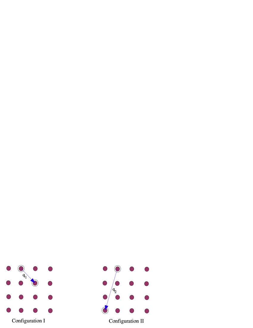
Figure 2: Two possible configurations for extra bosons in an incommensurate lattice.

If only onsite interactions are taken into account, the two configurations are degenerate. In the case of $m$ extra bosons, the degeneracy is $\frac{N!}{m!(N-m)!}$. The interbosonic distance is different for each degenerate configuration. Since there is no preferred distance, the extra bosons will not be initially trapped. If the well depth keeps increasing, the extra bosons will eventually be trapped too. But they will do so with many different wavevectors ${\vec{q}}_{i}$. The structure formed will be an amorphous solid.

In real life, besides on site interactions, there are interactions acting at long distances. They can be attractive or repulsive. These interactions are weaker than the on site interaction $U$, hence not important for a commensurate system. But if there is incommensuration, these interactions will probably play a role in determining the positions of the extra bosons. Another possibility is that when increasing $U$ the extra bosons get trapped in one of the possible configurations. If the configurations are metastable, then the system will remain there for a long time.

In our previous work, we had determined that a Mott localization transition could happen for incommensurate values of the number of bosons per site us . The nature of what this phase was was not elucidated. The difficulty lied in where to place the extra bosons after the integer part was subtracted from the total. As far as the Mott phase was concerned, they could fall in the wells at random as long as not two of them lie in the same well, for this would cost extra $U$’s of energy. In real life, an extra interaction might cause them to order in a certain way and decide the positions where they lie. We do not consider such a case here. Another possibility in the Bose-Hubbard model is that the integer part of the number of bosons per site (which is commensurate by definition) gets localized in each well and the leftover fraction constitute a Bose fluid. This would correspond to Mott-superfluid coexistence. We find that no such coexistence is possible.

When the total number of bosons is very near a commensurate number, the few leftover bosons are not localized and gain kinetic energy by being spread through the lattice. On the other hand, we do not think this constitutes a phase where we have coexistence of two phases. This is because the fraction of bosons which can be spread over the lattice collapses to zero as the lattice is made larger and larger. A true thermodynamic phase survives the thermodynamic limit. In fact, its properties become exact in the thermodynamic limit. Hence, the region where the fraction of bosons is free over the lattice exists only due to finite size effects. We thus conclude that for incommensurate values there is a Mott phase where the fraction of bosons that causes the incommensuration gets localized at random places in the lattice, forming a kind of amorphous solid.

We now estimate how this comes about. We will study, making mean field estimations, whether it is energetically favorable for the ground state to have all the bosons localized, or to have a commensurate number localized with the leftover fraction forming a gas or fluid coexisting with the Mott phase. The coexisting fluid will of course be a superfluid because of the repulsion, but we will only consider the fluid to be a Bose condensed free boson gas as a precondition for superfluidity is to have a Bose condensate.

In both the Mott phase with all the bosons localized and the phase with coexistence of the BEC and the Mott insulator (MI), we have $\sum_{i}\langle n_{i}\rangle=M$. Therefore, the chemical potential term will not favor any of the phases. In this section it will be dropped from our Bose Hubbard Hamiltonian for energetic comparisons:

$$\sum_{<ij>}-t\left(a_{i}^{\dagger}a_{j}+a_{j}^{\dagger}a_{i}\right)+U\sum_{i}n_{i}^{2}\;.$$ (66)

Without loss of generality we will consider the case where $M$ lies between $N$ and $2N$, which we parametrize as $M=(1+p)N$ with $0\leq p\leq 1$. The wavefunction that describes the Mott phase with all particles localized is given by

$$|\Psi_{M}\rangle=\prod_{i=1}^{M}a_{j_{i}}^{\dagger}|0\rangle$$ (67)

where the $j_{i}$’s run over lattice sites and the lattice sites are filled such that there is not less than one and not more than two particles per site. This way we have the minimum Hubbard energy possible. The expected value of the kinetic energy in this state is zero. Hence, the expected energy of this state is

$$E_{GS}^{M}=(3M-2N)U=UN(1+3p)\;.$$ (68)

This follows straightforwardly because we have $M-N$ sites with two particles at an energy cost $4U$, and $2N-M$ sites with one particle at an energy cost $U$.

For the phase consisting of the coexistence of a commensurate Mott phase ($N$ particles with one particle per well) with a BEC of the leftover $M-N$ particles the wavefunction is

$$|\Psi_{MB}\rangle=(a_{0}^{\dagger})^{M-N}\prod_{i=1}^{N}a_{i}^{\dagger}|0\rangle$$ (69)

where $a_{0}^{\dagger}$ is the operator that creates a boson with momentum $\vec{k}=0$. $a_{0}^{\dagger}=(1/\sqrt{N})\sum_{i}a_{i}^{\dagger}$. Only the fluid particles contribute to the expected value of the kinetic energy, which is given by

$$\langle E_{k}\rangle=-6t(M-N)\;.$$ (70)

In order to estimate the expected value of the interaction energy, we need to make a few estimates. The Mott component of this coexistence phase has exactly one particle per well. The fluid component, of course, has a fluctuating number of particles per well, whose average is $(M-N)/N$ leading to

$$\langle n_{i}\rangle=1+\frac{M-N}{N}=\frac{M}{N}\;.$$ (71)

In order to estimate the expected value of $n_{i}^{2}$, we reckon the following way: the Mott component of the coexistence phase does not have particle number fluctuations per site, leading to $(\Delta n_{i}^{2})_{M}=0$. The BEC component of the coexistence phase has fluctuations per site leading to typical fluctuations of a random liquid (classical or quantum) $(\Delta n_{i}^{2})_{MB}=(M-N)^{2}/N$. This number comes about because there is a quantum amplitude for all the fluid particles to be at each well (this is what it means to be fluid or delocalized). Hence, all the particles contribute to $\Delta n_{i}^{2}$ such that $\Delta n_{i}^{2}\propto(M-N)^{2}$. This needs to be multiplied by the probability of finding a particle in the well, which is $1/N$. The total fluctuations are given by quadrature: $\Delta n_{i}^{2}=(\Delta n_{i}^{2})_{M}+(\Delta n_{i}^{2})_{MB}$. From this we immediately obtain

$$\langle n_{i}^{2}\rangle=\Delta n_{i}^{2}+\langle n_{i}\rangle^{2}=\frac{(M-N)^{2}}{N}+\frac{M^{2}}{N^{2}}=p^{2}N+(1+p)^{2}\;.$$ (72)

The energy of the coexistence phase is

$$E_{GS}^{MB}=-6tNp+UN[(N+1)p^{2}+2p+1]\;.$$ (73)

We define the quantity

$$\frac{E_{GS}^{MB}-E_{GS}^{M}}{NU}=-\left(\frac{6t}{U}+1\right)p+(N+1)p^{2}$$ (74)

which when positive, the Mott phase is stable and when negative, the coexistence phase is stable. It follows that for $p$ between 0 and $((6t/U)+1)/(N+1)$ the coexistence phase is stable while for $p>((6t/U)+1)/(N+1)$ the incommensurate Mott phase is stable.

We see that when $N$ bosons get localized into a Mott phase with a single boson per site, the extra bosons one adds on top of these will gain more kinetic energy by delocalizing than the potential energy penalty coming from the overlap with the localized particles. Hence, they form a sort of fluid. The potential energy cost becomes too much when there is a fraction $p=((6t/U)+1)/(N+1)$. At this point they will localize too. This will happen despite there being an incommensurate number of them. In the absence of other long range interactions to tell the extra bosons where to localize, they will localize in random wells as long as no two of them go to the same well. For macroscopic lattices we see that the fraction of bosons that will delocalize becomes arbitrarily small. Therefore, this is a finite lattice size effect and does not reflect the properties of a true thermodynamic phase of matter, which by definition becomes better defined in the macroscopic limit.

VI Josephson vs. Individual Bosons Tunneling

In order to clarify the difference between the Mott phase we have uncovered and that of earlier work, we study BEC tunneling in an optical lattice. It has been verified experimentally in one dimensional optical lattices that there is coherent quantum tunneling in BEC’sbecj . We will try to take an in-depth look at tunneling in optical lattices in a general number of dimensions. Of course, the more relevant cases to superfluid-Mott transitions are those of higher dimensions, as superfluid ordering cannot occur in one dimension (see Appendix F). In order for the tunneling to be relevant, the hopping or tunneling energy scale, $t$, needs to be larger than the kinetic energy scale for the whole lattice:

$$T_{L}=\frac{\hbar^{2}}{2m\Omega^{2/3}}$$ (75)

where $m$ is the mass of the bosons and $\Omega$ is the volume of the whole lattice. If the kinetic energy of the lattice overwhelms the hopping, the tight-binding approximation with bosons hopping from lattice site to lattice site with tunneling $t$ is no longer valid for delocalized bosons.

On dimensional grounds one expects the tunneling rate to be proportional to $t/\hbar$. On the other hand, the proportionality factor should be a universal dimensionless function of the number of lattice sites $N$, the number of bosons $M$ and/or the number of bosons in the condensate $M_{0}$, and the different energy scales in the problem. Besides $t$ and $\hbar^{2}/2m\Omega^{2/3}$, there is the on-site repulsion at each well $U$, the well depth $\varepsilon$, and the kinetic energy scale of each well:

$$T_{w}=\frac{\hbar^{2}}{2mV^{2/3}}$$ (76)

where $V$ is the volume of each well $\sim a^{3}$ with $a$ the interlattice spacing. We, of course, have $NV=\Omega$. The wells are taken as large boxes. This approximation is valid as wells in optical lattices are fairly large ($a\sim 100$’s of nm) in typical latticesari1 .

The interwell tunneling rate or particle current is

$$J=\frac{t}{\hbar}F\left(M_{0},N,\frac{t}{\varepsilon},\frac{t}{U},\frac{T_{w}}{U}\right)$$ (77)

The universal function $F$ will behave differently in different physical regimes. For example, if the wells are very deep, $\varepsilon\gg t$, the tunneling rate should be exponentially suppressed $t\sim\exp(-\alpha\varepsilon/t)$ with $\alpha$ a positive numerical constant. We will never write the dependence of the function $F$ on $t/\varepsilon$ because the only effect of $\varepsilon$ for the suppression of tunneling is through the decrease of $t$. The number of bosons in the condensate, $M_{0}$, is determined uniquely by the number of bosons $M$, and the repulsion $U$. We see that the relevant parameter that sets the scale for the interaction for the BEC is the combination $UM_{0}/N$. Hence the universal dimensionless function that determines the tunneling current enhancement does not depend on $U,M_{0}$ and $N$ independently, but rather

$$F\left(M_{0},N,\frac{t}{U},\frac{T_{w}}{U}\right)=F\left(\frac{tN}{UM_{0}},\frac{T_{w}N}{UM_{0}}\right)$$ (78)

We remind the reader that the dispersion relation for the superfluid is

$$E_{\vec{k}}\equiv\sqrt{\tilde{\epsilon}_{\vec{k}}^{2}-\frac{4U^{2}M_{0}^{2}}{N^{2}}}=\frac{\hbar k}{\sqrt{2m}}\sqrt{\frac{\hbar^{2}k^{2}}{2m}+\frac{4UM_{0}}{N}}$$ (79)

where we make the continuum approximation $\epsilon_{\vec{k}}=\hbar^{2}k^{2}/2m$. As $k\rightarrow 0$ the dispersion becomes phononic, which leads to dissipationless flow. The dispersion at large $k$ becomes $\hbar^{2}k^{2}/2m$, which leads to dissipative flow. Notice that the crossover between dissipative and nondissipative flow happens at $k\simeq\sqrt{8mUM_{0}/\hbar^{2}N}$. This defines the coherence length of the superfluid

$$\xi\simeq\sqrt{\frac{\hbar^{2}N}{8mUM_{0}}}\;.$$ (80)

When the system is probed at length scales $L>\xi$ it responds collectively as a superfluid, while at length scales $L<\xi$ it behaves like a gas of independent bosonic particles, thus responding dissipatively, or even not behaving like a fluid at all if the spacing between levels is relevant. We note that an infinite system would become superfluid for any $U$ no matter how small, as one can always go to a long enough length scale to see the system respond collectively as a superfluid. In here we do not have in mind infinite systems but finite wells of superfluid. In this case of finite systems, if the kinetic energy scale of the well, $T_{w}$, is greater than the effective interaction, $UM_{0}/N$, the system will not be a superfluid as the linear size of the system, $V^{1/3}$, is less than the coherence length of the superfluid. Independent of whether the bosons are superfluid in each well, the system could still be a superfluid within the whole lattice.

For the full lattice, when the kinetic energy scale is set by tunneling between sites ($\epsilon_{\vec{k}}\simeq tk^{2}a^{2}$), the coherence length is

$$\xi\simeq a\sqrt{\frac{Nt}{4M_{0}U}}\;.$$ (81)

The size of the lattice is, of course, $L=Na$ and the condition for superfluidity ($\xi<L$) is $U/t>1/4M_{0}N$. We see that either for a very large system ($N\rightarrow\infty$) or very large number of bosons ($M_{0}\rightarrow\infty$), it becomes arbitrarily easy to become superfluid in the sense that an arbitrarily small $U$ will order the boson fluid into a superfluid at low enough temperature. Conversely, as we make the system small, or we reduce the number of bosons, it becomes harder to order into a superfluid, which will show up experimentally as increased dissipation rates.

Even though a high enough $U$ can order the system into a superfluid, too high a $U$ will make it into a Mott insulatorfisher ; us . The transition to the Mott insulator can be continuousfisher or discontinuousus . The continuous transition occurs when there is a superfluidfisher in each well and $U$ prevents Josephson tunneling between wells. The continuous transition only happens for a commensurate number of bosons per site. When the bosons in the wells are not superfluid within wells the transition is discontinuous and happens irrespective of whether the number of bosons per site is integer or notus . The second transition always happens when the number of bosons per site or $U/t$ are sufficiently small as in these cases $\xi>a$. In fact from our estimate (81) there cannot be a superfluid within each well when

$$\frac{Nt}{4M_{0}U}>1\;.$$ (82)

For this case the Mott transition will be like ours if this condition still holds at the critical value of $U/t$, otherwise the Mott transition will be that of suppression of Josephson tunnelingfisher .

We now proceed to consider the case when there is a superfluid within each well. This will elucidate the microscopic physics of how onsite repulsion suppresses Josephson tunneling, leading to the transition studied by Fisher, et. al. fisher . We will see that commensuration plays no role in the suppression of tunneling. This leads us to suspect that a first order transition can occur for this case too contrary to the early work fisher . The reason this was not found out in that work is that they perform renormalization group studies which can only access continuous transitions. Whether a discontinuous transition can occur in this case is a matter for further study.

We evaluate the current operatorjoseph

$$\hat{J} \equiv\frac{d}{dT}(N-\bar{N})=-\frac{i}{\hbar}\left[N-\bar{N},H_{t}\right]$$

$$=-\frac{2it}{\hbar}\sum_{\vec{k}}\left(a_{\vec{k}}^{\dagger}\bar{a}_{\vec{k}}-\bar{a}_{\vec{k}}^{\dagger}a_{\vec{k}}\right)$$ (83)

where

$$H_{t}=-t\sum_{\vec{k}}\left(a_{\vec{k}}^{\dagger}\bar{a}_{\vec{k}}+\bar{a}_{\vec{k}}^{\dagger}a_{\vec{k}}\right)$$ (84)

is the tunneling part of the Hamiltonian and $T$ denotes time. Now $a_{\vec{k}}$ and $\bar{a}_{\vec{k}}$ are boson operators for different adjacent wells. At first we consider the tunneling current when we have a superfluid within each well. We note that the ground state of the reduced Hamiltonian (14) when $t=0$ is an outer product of the Bogolyubov ground states for each well, which we denote as our “vacuum” state $|\psi_{0}\rangle$. The excited states of such a system are denoted by $|n\rangle$ and are constructed by applying any number of Bogolyubov creation operators to the vacuum state. The energies of such states, $E_{n}$, will be the sum of the energies of each of the operators. When $t\neq 0$ there will be tunneling between adjacent wells, which can be calculated accurately from linear response theory pines as long as the number of atoms within the wells is large. For such a calculation the only relevant excited states are two quasiparticle states, one in each adjacent well, with opposite momenta, i.e. $|n\rangle=\bar{b}_{\vec{k}}^{\dagger}b_{-\vec{k}}^{\dagger}|\psi_{0}\rangle$, with energies $E_{n}=2E_{\vec{k}}$. This calculation was first done by B. D. Josephson for Cooper paired fermionic superconductorsjoseph . We will follow his calculation closely. When the wells are superfluid, the tunneling current is dominated by coherent tunneling of Bogolyubov correlated pairs.

In order to calculate in linear response theorypines , we turn on $H_{t}$ adiabatically from time $T=-\infty$, starting from the ground state of the noninteracting system at such a time. If we expand the wavefunction in terms of the noninteracting eigenstates

$$|\Psi\rangle=\sum_{n}a_{n}(T)\exp{(-iE_{n}T/\hbar)}|n\rangle$$

we obtain the well known formula

$$a_{n}(T)=\delta_{n,0}-i\exp{(iE_{n}T/\hbar)}\langle n|H_{t}|\psi_{0}\rangle/(iE_{n}+\epsilon)$$ (85)

where the vacuum state energy $E_{0}$ has been chosen to be 0. The parameter $\epsilon$ was introduced to control the adiabatic switching of the interaction. The causal limit $\epsilon\rightarrow 0^{+}$ should be always understood. Our interaction is turned on fully at time $T=0$ and the wavefunction of the interacting system is given by $|\Psi(0)\rangle=|\psi_{0}\rangle+|\delta\varphi\rangle$ wherepines

$$|\delta\varphi\rangle=-\sum_{n\neq 0}\frac{|n\rangle\langle n|H_{t}|\psi_{0}\rangle}{E_{n}-i\epsilon}$$ (86)

The Josephson current is given by $\langle\Psi(0)|\hat{J}|\Psi(0)\rangle=\langle 0|\hat{J}|\delta\varphi\rangle+$ complex conjugate. With

$$|\delta\varphi\rangle=t\sum_{\vec{k}}\frac{u_{\vec{k}}v_{\vec{k}}}{2E_{\vec{k}}-i\epsilon}\left(e^{-i\theta}b_{\vec{k}}^{\dagger}\bar{b}_{-\vec{k}}^{\dagger}+b_{-\vec{k}}^{\dagger}\bar{b}_{\vec{k}}^{\dagger}\right)\;,$$ (87)

where $\theta$ is the phase difference between the superfluid order parameters in adjacent wells, we obtain

$$J=-\frac{2t^{2}}{\hbar}\sin{\theta}\sum_{\vec{k}}\frac{u_{\vec{k}}^{2}v_{\vec{k}}^{2}}{E_{\vec{k}}}$$ (88)

analogous to the fermionic superconducting case joseph . We note that if $\theta$ is 0 there is no Josephson tunneling as the superfluids are in phase. Since $u_{\vec{k}}v_{\vec{k}}=UM_{0}/E_{\vec{k}}N$, we obtain for the enhancement factor $F=J\hbar/t$

$$F=-\frac{2tU^{2}M_{0}^{2}}{N^{2}}\sin{\theta}\sum_{\vec{k}}\frac{1}{E_{\vec{k}}^{3}}$$ (89)

In order to estimate this quantity we approximate the quasiparticle dispersion as phononic, $E_{\vec{k}}^{2}\simeq 2UM_{0}\hbar^{2}k^{2}/mN$, and we cut off the high momenta at $k_{c}$ of the order of the inverse coherence length. Converting the sum into an integral

$$\sum_{\vec{k}}\frac{1}{E_{\vec{k}}^{3}}\simeq\frac{1}{(2\pi)^{3}}\left(\frac{mNV^{2/3}}{2UM_{0}}\right)^{3/2}\int_{k<k_{c}}\frac{d^{3}\vec{k}}{k^{3}}$$ (90)

Note that this integral is infrared divergent but the divergence gets cut-off by the inverse linear well size $V^{1/3}$. We finally obtain for the enhancement

$$F=\frac{1}{16\pi^{2}}\frac{tN}{UM_{0}}\left(\frac{UM_{0}}{T_{w}N}\right)^{3/2}\;\ln{\frac{4UM_{0}}{T_{w}N}}$$ (91)

In order for the system to be superfluid at all within a well we must have the linear dimensions of the well larger than the coherence length, $V^{1/3}>\xi$, and there needs to be enough bosons in each well as to have superfluid broken symmetry. Otherwise, there will not be Josephson tunneling per se and the calculation of tunneling will have to be done for noninteracting bosons trapped in wells. This condition is $UM_{0}/T_{w}N>1/4$ with smaller values corresponding to a physically impossible regime. When the conditions are such that there can be Josephson tunneling between sites, intrawell Coulomb repulsion will suppress Josephson tunneling, leading to a Mott insulating phase as studied originally fisher . On the other hand, when Josephson tunneling cannot occur from well to well because the coherence length is longer than the well size, the Mott transition will be single boson localization as uncovered by us us . The conditions in Mott transitions in optical lattice experiments ib ; ari are such that the coherence length is too long and the number of bosons too few as to support Josephson tunneling between adjacent wells as there would not be a superfluid within each well.

We concentrate on the case when the linear size of the wells is too small ($V^{1/3}<\xi$). In this case the interaction cannot order the system into a superfluid within each well (although it can certainly be a superfluid within the whole lattice), and its only effect is a renormalization of the mass of the bosons. Hence the system is described by the Hamiltonian (84) with $m$ the renormalized mass of the bosons. There is no Josephson tunneling per se as the system is not superfluid. On the other hand, there can be coherent quantum tunneling of the (nonsuperfluid) boson liquid between wells.

The Hamiltonian (84) is diagonalized by the canonical operators

$$A_{\vec{k}}=\frac{a_{\vec{k}}+\bar{a}_{\vec{k}}}{\sqrt{2}}\qquad\bar{A}_{\vec{k}}=\frac{a_{\vec{k}}-\bar{a}_{\vec{k}}}{\sqrt{2}}$$ (92)

to yield

$$\mathcal{H}=\sum_{\vec{k}}\left\{(\epsilon_{\vec{k}}-t)A_{\vec{k}}^{\dagger}A_{\vec{k}}+(\epsilon_{\vec{k}}+t)\bar{A}_{\vec{k}}^{\dagger}\bar{A}_{\vec{k}}\right\}$$ (93)

The Heisenberg equations of motion lead to the following time dependent operators $A_{\vec{k}}(T)=A_{\vec{k}}\exp[-i(\epsilon_{\vec{k}}-t)T/\hbar]$ and $\bar{A}_{\vec{k}}(T)=\bar{A}_{\vec{k}}\exp[-i(\epsilon_{\vec{k}}+t)T/\hbar]$. The common phase factor $-i\epsilon_{\vec{k}}T/\hbar$ will be dropped as only phase differences affect the physics. From these time dependent operators one immediately obtains the operators into which $a_{\vec{k}}$ $\bar{a}_{\vec{k}}$ and their conjugates develop under Hamiltonian evolution:

$$a_{\vec{k}}(T)=\cos\left(\frac{tT}{\hbar}\right)a_{\vec{k}}+i\sin\left(\frac{tT}{\hbar}\right)\bar{a}_{\vec{k}}$$

$$\bar{a}_{\vec{k}}(T)=\cos\left(\frac{tT}{\hbar}\right)\bar{a}_{\vec{k}}+i\sin\left(\frac{tT}{\hbar}\right)a_{\vec{k}}$$

$$a_{\vec{k}}^{\dagger}(T)=\cos\left(\frac{tT}{\hbar}\right)a_{\vec{k}}^{\dagger}-i\sin\left(\frac{tT}{\hbar}\right)\bar{a}_{\vec{k}}^{\dagger}$$

$$\bar{a}_{\vec{k}}^{\dagger}(T)=\cos\left(\frac{tT}{\hbar}\right)\bar{a}_{\vec{k}}^{\dagger}-i\sin\left(\frac{tT}{\hbar}\right)a_{\vec{k}}^{\dagger}$$ (94)

The “barred” and “unbarred” operators are orthogonal raising and lowering operators as unitary Hamiltonian evolution is a canonical transformation thus preserving the commutation relations of the operators at time zero.

We can now calculate the coherent tunneling current between two wells. We take the right well to have $(N+M)/2$ bosons and the left well with $(N-M)/2$ bosons. The initial wavefunction is then

$$|\Psi(0)\rangle=\Big{[}\frac{(a_{0}^{\dagger})^{(N+M)/2}(\bar{a}_{0}^{\dagger})^{(N-M)/2}}{(N/2+M/2)!(N/2-M/2)!}\Big{]}|\psi_{0}\rangle$$ (95)

where the subscript $0$ means the smallest momentum state into which the bosons condensed. The wavefunction at time $T$, $|\Psi(T)\rangle$, has the exact same dependence on the operators $a_{0}^{\dagger}(T)$, $\bar{a}_{0}^{\dagger}(T)$ that $|\Psi(0)\rangle$ has on $a_{0}^{\dagger}$, $\bar{a}_{0}^{\dagger}$. In order to obtain the coherent tunneling current $J$ we need to evaluate $\langle\Delta N(T)\rangle\equiv\langle\Psi(T)|\Delta N|\Psi(T)\rangle$ with $\Delta N\equiv a_{0}^{\dagger}a_{0}-\bar{a}_{0}^{\dagger}\bar{a}_{0}$ counting the excess number of bosons in the right well. Using

$$\Delta N=\cos\left(\frac{2tT}{\hbar}\right)(a_{0}^{\dagger}(T)a_{0}(T)-\bar{a}_{0}^{\dagger}(T)\bar{a}_{0}(T))$$

$$+2i\sin\left(\frac{2tT}{\hbar}\right)(\bar{a}_{0}^{\dagger}(T)a_{0}(T)-a_{0}^{\dagger}(T)\bar{a}_{0}(T))$$ (96)

we obtain the tunneling current

$$J=\frac{d}{dT}\langle\Delta N(T)\rangle=\frac{2t}{\hbar}M\sin\left(\frac{2tT}{\hbar}\right)$$ (97)

where the periodicity is an artifact of having a two site system. The proportionality of the tunneling current on the initial number difference of bosons between the sites, $M$, is not an artifact. This coherent quantum tunneling can and will be suppressed by strong enough repulsion within the wells, leading to boson localization within the wells.

Before concluding we will make some order of magnitude estimate of when the Mott transition happens. Let us first consider the case when the coherence length is smaller than the well size and there is a macroscopic number of bosons per well such that there can be a superfluid within each well. In this case, the Mott transition will be suppression of Josephson tunneling as studied theoretically before the advent of BECs fisher . In this case, the energy scale associated with tunneling is the Josephson tunneling energy

$$E_{J}=t\frac{1}{16\pi^{2}}\frac{t}{T_{w}}\left(\frac{UM_{0}}{T_{w}N}\right)^{1/2}\;\ln{\frac{4UM_{0}}{T_{w}N}}$$ (98)

where $4UM_{0}\ T_{w}N>1$ for Josephson tunneling to be possible. When the average Hubbard repulsion energy per site, $E_{U}=U(M_{0}/N)^{2}$, is larger than the Josephson energy the Hubbard interaction prevents tunneling, making the system into a Mott insulator. Since we expect the logarithm not to deviate much from factors of order 1, we can estimate this condition to be about

$$\left(\frac{t}{T_{w}}\right)^{2}\left(\frac{UM_{0}}{T_{w}N}\right)^{-1/2}\sim\frac{M_{0}}{N}$$ (99)

For the case of long coherence length or few bosons per site, the transition will be individual boson localization with suppression of individual boson tunneling rather than Josephson tunneling. The energy scale for individual boson tunneling is set roughly by $t$. We would expect the transition to the Mott phase to happen when this energy is swamp by the Hubbard interaction energy

$$\frac{U}{t}\sim\frac{N}{M_{0}}$$ (100)

which is very roughly a condensate depletion condition. When the lattice tunneling is more relevant than the intra-well kinetic energy, $t>T_{W}$ and the number of bosons per site is of order 1, the boson localization phase transition described in this work will happen. On the other hand, if $t<T_{W}$ or the number of bosons per site is considerably greater than one, one expects a Mott transition with suppression of Josephson tunneling and superfluidity within each well. If the number of bosons per site is considerably less than one, one can probably not speak of either transition.

VII Conclusion

In BEC’s in an optical lattice the Mott transition is induced by making the wells on the lattice sites deeper ($\varepsilon$ is the lattice depth) thus suppressing the tunelling amplitude $t$ between near neighbor sites, i.e. making the bosons “heavy”. Thus the relevant ratio of on-site repulsion $U$ to hopping $t$ increases. As this ratio increases, the superfluid order parameter increases as shown in the figure 1. The increase of the order parameter means that the superfluid phase is becoming more stable over the Bose condensed gas. On the other hand, we also plot the number of particles in the condensate. This number is becoming small as $U/t$ increases. As the condensate gets depleted the system is becoming “less fluid” and will solidify into a Mott insulating phase with a well defined number of bosons per site. When the coherence length is longer than the interwell spacing, or the number of bosons per well too small, the Bogolyubov order parameter will be zero within each well and in the quantum solid phase. There will be a discontinuous jump in the superfluid response at the Mott transition. This transition can happen regardless of commensuration and the conditions in most lattice experiments are conducive to this transition ib ; ari .

The physics of the transition we have described in the present work differs considerably from the one proposed in the pioneering theoretical work on Bose systems fisher and thus requires some comments. The first and, perhaps, most important difference is that we do not consider a phase only model as it is not appropriate to the Mott insulator at low densities since a superfluid order parameter cannot survive within each well. In that original work, the phase of the superfluid was disordered by the increasing repulsion thus leading to a transition. In such a transition the solid would have a superfluid order parameter within each well, but the phase of the order parameter will have become randomized exactly analogous to what happens in Josephson junction arrays when the charging energy is sufficiently large. Such an insulating phase does not correspond to the Mott insulator we studied here and cannot exist at small number of bosons per site as one needs a macroscopic number of particles to have a superfluid order parameter. It can also not exist when the coherence length of the superfluid is longer than the well size. Finally, we stress that the phase only model studied in the early work fisher ; ja is a correct model of an array of Josephson coupled superfluid systems and should work for bosons in an optical lattice when the number of bosons per site is large enough, and the coherence length short enough as to make superfluid order within each well possible. Josephson coupled systems can easily be studied in an optical lattice mark1 ; becj . It will be extremely interesting to see what the experimental phase diagram turns out to be.

Appendix A Derivation of the Bogolyubov Hamiltonian

The interaction part of the Hamiltonian can be written as

$$\mathcal{H}_{int}=\frac{U}{N}\sum_{{\vec{k}},{\vec{k}}_{2},{\vec{q}}}\;a_{{\vec{k}}+{\vec{q}}}^{\dagger}\;(a_{{\vec{k}}_{2}-{\vec{q}}}^{\dagger}a_{\vec{k}}+\delta_{{\vec{k}},{\vec{k}}_{2}-{\vec{q}}})\;a_{{\vec{k}}_{2}}$$

$$\mathcal{H}_{int}=\frac{U}{N}\sum_{{\vec{k}},{\vec{k}}_{2},{\vec{q}}}\;a_{{\vec{k}}+{\vec{q}}}^{\dagger}a_{{\vec{k}}_{2}-{\vec{q}}}^{\dagger}a_{\vec{k}}a_{{\vec{k}}_{2}}+\frac{U}{N}\sum_{{\vec{k}},{\vec{q}}}a_{\vec{k}}^{\dagger}a_{\vec{k}}$$ (101)

$$=\mathcal{H}_{I}+\frac{U}{N}\sum_{{\vec{k}},{\vec{q}}}a_{\vec{k}}^{\dagger}a_{\vec{k}}$$

Now we start analyzing terms from $\mathcal{H}_{I}$. Separating from the momentum sums all the terms with $a_{0}$ or $a_{0}^{\dagger}$ and replacing the values of these operators by $\sqrt{M_{0}}$ since the condensate is macroscopically occupied and these operators behave like c-numbers, we get

$$\mathcal{H}_{I}=\frac{UM_{0}^{2}}{N}+\frac{4UM_{0}}{N}\sum_{{\vec{k}}\neq 0}a_{\vec{k}}^{\dagger}a_{\vec{k}}+\frac{2U\sqrt{M_{0}}}{N}\sum_{{\vec{k}}_{2}\neq 0,\vec{q}}\sum_{{\vec{q}}\neq 0}\;\left(a_{\vec{q}}^{\dagger}a_{{\vec{k}}_{2}-{\vec{q}}}^{\dagger}a_{{\vec{k}}_{2}}+a_{{\vec{k}}_{2}}^{\dagger}a_{{\vec{k}}_{2}-{\vec{q}}}a_{\vec{q}}\right)\\ +\frac{UM_{0}}{N}\sum_{{\vec{q}}\neq 0}\;\left(a_{\vec{q}}^{\dagger}a_{-{\vec{q}}}^{\dagger}+a_{-{\vec{q}}}a_{\vec{q}}\right)+\frac{U}{N}\sum_{{\vec{k}}_{2}\neq 0,\vec{q}}\sum_{{\vec{k}}\neq 0,-\vec{q}}\sum_{\vec{q}}\;a_{{\vec{k}}+{\vec{q}}}^{\dagger}a_{{\vec{k}}_{2}-{\vec{q}}}^{\dagger}a_{\vec{k}}a_{{\vec{k}}_{2}}$$ (102)

We concentrate on the universal ground state and low energy properties of the superfluid. We thus neglect the terms with factors of $\sqrt{M_{0}}$ or smaller since the macroscopic occupation of the condensate will make them unimportant. We arrive then at the reduced Bogolyubov Hamiltonian

$$\mathcal{H}_{bog}=\frac{UM_{0}^{2}}{N}+\sum_{\vec{k}\neq 0}\tilde{\epsilon}_{\vec{k}}\;a_{\vec{k}}^{\dagger}a_{\vec{k}}\\ +\frac{UM_{0}}{N}\sum_{{\vec{k}}\neq 0}\;(a_{\vec{k}}^{\dagger}a_{-{\vec{k}}}^{\dagger}+a_{-{\vec{k}}}a_{\vec{k}})$$ (103)

where

$$\tilde{\epsilon}_{\vec{k}}=\epsilon_{\vec{k}}+(4UM_{0}/N)-\mu\;.$$ (104)

The extra term $\frac{U}{N}\sum_{{\vec{k}},{\vec{q}}}a_{\vec{k}}^{\dagger}a_{\vec{k}}$ in equation (101) can be written as $U\sum_{\vec{k}}a_{\vec{k}}^{\dagger}a_{\vec{k}}$. In this way, it is seen that such a term just renormalizes the chemical potential. It has therefore been absorbed into $\mu$.

Appendix B Bosonic Superfluid Ground State

The manipulations reviewed in the present appendix are original to Bogolyubov bog and we follow closely K. Huanghuang The ground state wavefunction for the Bogolyubov Hamiltonian (14) has the form

$$|\Psi_{0}\rangle=\sum_{n_{1},m_{1}}\sum_{n_{2},m_{2}}\;...\;(c_{n_{1},m_{1}}c_{n_{2},m_{2}}\;...\;)|n_{1}m_{1};\;n_{2}m_{2};\;...\;\rangle$$ (105)

where $n_{i}$ is the number of particles with momentum ${\vec{k}}_{i}$ and $m_{i}$ is the number of particles with momentum $-{\vec{k}}_{i}$. It is obviously the state with no excitations

$$b_{\vec{k}}|\Psi_{0}\rangle=(u_{\vec{k}}a_{\vec{k}}+v_{\vec{k}}a_{-{\vec{k}}}^{\dagger})|\Psi_{0}\rangle=0$$

Let $c_{n,m}=c_{n_{1},m_{1}}c_{n_{2},m_{2}}\;...\;$, $u=u_{\vec{k}}$, $v=v_{\vec{k}}$ and $|n,m\rangle=|n_{1}m_{1};\;n_{2}m_{2};\;...\;\rangle$. Then

$$\sum_{n,m}(u\;c_{n,m}\sqrt{n}\;|n-1,m\rangle+v\;c_{n,m}\sqrt{m+1}\;|n,m+1\rangle)=0$$ (106)

Changing dummy variables $n\rightarrow n+1$ in the first term of the sum and $m\rightarrow m-1$ in the second term

$$\sum_{n,m}(u\;c_{n+1,m}\sqrt{n+1}+v\;c_{n,m-1}\sqrt{m})\;|n,m\rangle=0$$ (107)

For $n\neq m$ and $m=0$ we have

$$u\;c_{n+1,m}\sqrt{n+1}\;+\;v\;c_{n,m-1}\sqrt{m}=0$$

$$c_{n+1,0}=0\quad\text{for all $n$'s}$$

for m = 1

$$u\;c_{n+1,1}\sqrt{n+1}\;+\;v\;c_{n,0}=u\;c_{n+1,1}\ sqrt{n+1}=0$$

$$c_{n+1,1}=0$$

and so on for all $c_{n,m}$. Thus we only need to consider $n=m$ in $c_{n,m}$. In that case we have from (107)

$$u\;c_{m,m}\;+\;v\;c_{m-1,m-1}=0$$

$$c_{m,m}=-\frac{v}{u}c_{m-1,m-1}=(-\frac{v}{u})^{2}c_{m-2,m-2}=(-\frac{v}{u})^{3}c_{m-3,m-3}$$

$$c_{m,m}=(-\frac{v}{u})^{m}c_{0,0}$$ (108)

Substituting this into (105) we find

$$|\Psi_{0}\rangle=\prod_{\vec{k}}\sum_{n=0}^{\infty}(-\frac{v_{\vec{k}}}{u_{\vec{k}}})^{n}c_{0,0}|n,n\rangle$$ (109)

where we can write the state composed of n particles with momentum ${\vec{k}}$ and n particles with momentum $-{\vec{k}}$ as

$$|n,n\rangle=\frac{(a_{\vec{k}}^{\dagger})^{n}}{\sqrt{n!}}\frac{(a_{-{\vec{k}}}^{\dagger})^{n}}{\sqrt{n!}}\;|0\rangle$$ (110)

hence

$$|\Psi_{0}\rangle=\prod_{\vec{k}}\sum_{n=0}^{\infty}(-\frac{v_{\vec{k}}}{u_{\vec{k}}})^{n}c_{0,0}\frac{(a_{\vec{k}}^{\dagger})^{n}(a_{-{\vec{k}}}^{\dagger})^{n}}{n!}\;|0\rangle$$ (111)

$$|\Psi_{0}\rangle=\prod_{\vec{k}}c_{0,0}e^{-\frac{v_{\vec{k}}}{u_{\vec{k}}}a_{\vec{k}}^{\dagger}a_{-{\vec{k}}}^{\dagger}}|0\rangle$$ (112)

which is a coherent state. We need to find the normalization constant $c_{0,0}$. Notice that

$$\langle\Psi_{0}|\Psi_{0}\rangle=|c_{0,0}|^{2}\langle 0|e^{\frac{-v_{\vec{k}}}{u_{\vec{k}}}a_{\vec{k}}a_{-{\vec{k}}}}e^{\frac{-v_{\vec{k}}}{u_{\vec{k}}}a_{\vec{k}}^{\dagger}a_{-{\vec{k}}}^{\dagger}}|0\rangle$$

$$\langle\Psi_{0}|\Psi_{0}\rangle=|c_{0,0}|^{2}\sum_{n,m}(-1)^{n+m}(\frac{v_{\vec{k}}}{u_{\vec{k}}})^{n+m}\\ \times\frac{\langle 0|a_{\vec{k}}^{n}a_{-{\vec{k}}}^{n}(a_{\vec{k}}^{\dagger})^{m}(a_{-{\vec{k}}}^{\dagger})^{m}|0\rangle}{n!m!}$$

and furthermore

$$\langle 0|a_{\vec{k}}^{n}a_{-\vec{k}}^{n}(a_{\vec{k}}^{\dagger})^{m}(a_{-\vec{k}}^{\dagger})^{m}|0\rangle=\delta_{n,m}\langle 0|a_{\vec{k}}^{n}a_{-\vec{k}}^{n}(a_{\vec{k}}^{\dagger})^{n}(a_{-\vec{k}}^{\dagger})^{n}|0\rangle$$

$$a_{-\vec{k}}^{\dagger}|0\rangle=\sqrt{1}|1,0\rangle\qquad(a_{-\vec{k}}^{\dagger})^{2}|0\rangle=\sqrt{1}\sqrt{2}|2,0\rangle$$

$$(a_{-\vec{k}}^{\dagger})^{n}|0\rangle=\sqrt{n!}|n,0\rangle(a_{\vec{k}}^{\dagger})^{n}|0\rangle=\sqrt{n!}|0,n\rangle$$

$$a_{-\vec{k}}|0\rangle=0\qquad a_{-\vec{k}}|n\rangle=\sqrt{n}|n-1\rangle$$

$$(a_{-\vec{k}})^{2}|n\rangle=\sqrt{n}\sqrt{n-1}|n-2\rangle\qquad(a_{-\vec{k}})^{n}|0\rangle=\sqrt{n!}|0\rangle$$

Using the expressions above we find

$$\langle 0|a_{\vec{k}}^{n}a_{-\vec{k}}^{n}(a_{\vec{k}}^{\dagger})^{n}(a_{-\vec{k}}^{\dagger})^{n}|0\rangle=n!\langle 0|a_{\vec{k}}^{n}a_{-\vec{k}}^{n}|n,n\rangle\\ =(n!)^{2}\langle 0|0\rangle=(n!)^{2}$$

which finally yields

$$\langle\Psi_{0}|\Psi_{0}\rangle=|c_{0,0}|^{2}\sum_{n,m}\frac{(-1)^{n+m}(\frac{v_{\vec{k}}}{u_{\vec{k}}})^{n+m}}{n!m!}\delta_{n,m}(n!)^{2}$$

$$=|c_{0,0}|^{2}\sum_{n}(\frac{v_{\vec{k}}}{u_{\vec{k}}})^{2n}=1$$

$$|c_{0,0}|^{2}=\frac{1}{\sum_{n}(\frac{v_{\vec{k}}}{u_{\vec{k}}})^{2n}}$$ (113)

Remembering that $\sum_{n}(\frac{v_{\vec{k}}^{2}}{u_{\vec{k}}^{2}})^{n}=\frac{1}{1-v_{\vec{k}}^{2}/u_{\vec{k}}^{2}}=u_{\vec{k}}^{2}$ we arrive at the expression $|c_{0,0}|^{2}=\frac{1}{u_{\vec{k}}^{2}}$. The normalized ground state wavefunction is then

$$\qquad\quad|\Psi_{0}\rangle=\prod_{\vec{k}}\frac{1}{u_{\vec{k}}}e^{-(v_{\vec{k}}/u_{\vec{k}})a_{\vec{k}}^{\dagger}a_{-\vec{k}}^{\dagger}}\;|0\rangle$$ (114)

Appendix C Universal Superfluid physics

In the present appendix we review and emphasize some of the hydrodynamic and universal properties of the superfluid phase as realized in Helium and BECs.

C.1 Rigidity and Superfluidity

We first review the Landau argument landau illustrating how the lack of rigidity causes dissipation. Consider a Bose fluid at zero temperature (a Bose condensate) with excitation spectrum given by $\epsilon_{\vec{p}}$. Suppose the fluid is moving with velocity $\mathbf{v}$ and interacts with something external (what does it interact with is irrelevant, but one could think that it is a surface over which it is moving).

The interaction can exchange energy and momentum with the fluid. The fluid has initial energy $Mv^{2}/2$ with $M$ the total mass of the fluid. The interaction creates a quasiparticle with energy $\epsilon_{\mathbf{p}}$ in the frame of the Bose fluid. In the lab frame the particle has energy

$$\tilde{\epsilon}_{\vec{p}}=\epsilon_{\vec{p}}+\vec{p}\cdot\vec{v}$$ (115)

by Galilean invariance since the velocity of the particle in the fluid frame is $\vec{v}_{\vec{p}}=\partial\epsilon_{\vec{p}}/\partial\vec{p}$ and it is $\vec{v}_{\vec{p}}+\vec{v}$ in the lab frame.

Energy will be exchanged if the fluid can lower its energy. The fluid final energy is

$$\frac{Mv^{2}}{2}+\epsilon_{\vec{p}}+\vec{p}\cdot\vec{v}\;$$ (116)

The condition for dissipation is thus $\epsilon_{\vec{p}}+\vec{p}\cdot\vec{v}<0$. The easiest way to satisfy the condition is when $\vec{p}$ is antiparallel to $\vec{v}$. We then obtain dissipation for

$$v>\left(\frac{\epsilon_{\vec{p}}}{p}\right)_{\text{min}}\;$$ (117)

We see that for all dispersions softer than sound the minimum on the right hand side of the last equation is zero and there is dissipation for any velocity of the fluid. If the dispersion is at least as stiff as sound, for velocities smaller than some critical velocity there is no dissipation and hence superflow. Since as long as the system is a quantum Bose fluid, i.e. there exists a condensate, repulsion produces sound excitations as the elementary low energy quasiparticles of the system, the interactions provide the necessary rigidity for superfluidity. The free Bose gas, despite the macroscopic coherent occupation of the lowest momentum state, is not a superfluid as it is arbitrarily easy to destroy its coherence no matter how weak the perturbation. In fact, at energy scales in which the superfluid behaves as a free Bose gas, it dissipates and it is not super at all. This happens for wavelengths shorter than the coherence length of the superfluid as explained in a subsequent section.

C.2 Scattering

The purpose of this section is to illustrate the principles of superfluidity and of macroscopic exactness by an example. Among the experimental efforts on BECs figure studies of spontaneous emission and light scattering of these superfluid systems by W. Ketterle and collaboratorskett1 . They found that light scattering off BECs is suppressed to negligible values at long wavelengths. This seems surprising at first since one can naively expect the typical $n+1$ bosonic enhancementbec4 as observed in their emission experimentskett1 . They have attributed the observed suppression of light scattering in BECs to destructive quantum interference effectsbec4 . While their argument is certainly true, it is the purpose of this section to point out that the more universal reason that makes their argument, and hence their results, true is the Principle of Superfluidity. We show that the suppression of light scattering off a Bose Einstein Condensate is equivalent to the Landau argument for superfluidity and thus is a consequence of the Principle of Superfluidity. This means that the superfluidity is ultimately the reason for suppressed scattering at low wavelengths. We have previously presented these arguments in a short notenos .

We will study next scattering processes in the superfluid. In a scattering event, an incoming particle couples to the density of the system. The effective scattering Hamiltonian is

$$\mathcal{H}_{I}=\int d^{3}rV({\bf r},t)\rho({\bf r})+\text{H.C.}$$ (118)

where by Fourier transforming

$$V({\bf r},t)=\sum_{\vec{q}}V_{\vec{q}}e^{-i({\vec{q}}\cdot{\bf r}-\omega t)}$$ (119)

Hence

$$\mathcal{H}_{I}=\sum_{\vec{q}}V_{\vec{q}}\int d^{3}r\;e^{-i({\vec{q}}\cdot{\bf r}-\omega t)}\rho({\bf r})+\text{H.C.}$$ (120)

$V_{\vec{q}}$ is the interaction matrix element between the final and initial states of the external particle. Now, $\rho_{\vec{q}}=\int d^{3}r\;\rho({\bf r})e^{-i{\vec{q}}\cdot{\bf r}}$ and at an arbitrary point $i$, the density is given by $\rho({\bf r}_{i})=a_{i}^{\dagger}a_{i}$, where

$$a_{i}=\sum_{\vec{k}}e^{-i{\vec{k}}\cdot{\bf r}}a_{\vec{k}}\qquad a_{i}^{\dagger}=\sum_{{\vec{k}}^{\prime}}e^{i{\vec{k}}^{\prime}\cdot{\bf r}}a_{{\vec{k}}^{\prime}}^{\dagger}$$ (121)

thus

$$\rho({\bf r})=\sum_{{\vec{k}},{\vec{k}}^{\prime}}e^{-i({\vec{k}}-{\vec{k}}^{\prime})\cdot{\bf r}}a_{{\vec{k}}^{\prime}}^{\dagger}a_{\vec{k}}$$ (122)

$$\int d^{3}r\;\rho({\bf r})e^{-i{\vec{q}}\cdot{\bf r}}=\sum_{{\vec{k}},{\vec{k}}^{\prime}}a_{{\vec{k}}^{\prime}}^{\dagger}a_{\vec{k}}\int e^{-i({\vec{q}}+{\vec{k}}-{\vec{k}}^{\prime})\cdot{\bf r}}\;d^{3}r\\ =\sum_{{\vec{k}},{\vec{k}}^{\prime}}a_{{\vec{k}}^{\prime}}^{\dagger}a_{\vec{k}}\;\delta({\vec{q}}+{\vec{k}}-{\vec{k}}^{\prime})=\sum_{\vec{k}}a_{{\vec{k}}+{\vec{q}}}^{\dagger}a_{\vec{k}}$$ (123)

and

$$\mathcal{H}_{I}=\sum_{\vec{k}}V_{\vec{q}}e^{i\omega t}a_{{\vec{k}}+{\vec{q}}}^{\dagger}a_{\vec{k}}+\text{H.C.}$$ (124)

where the energy and momentum transfered in the scattering event are

$$\vec{q}=\vec{q}_{f}-\vec{q}_{i}\;\;\text{and}\;\;\omega=\omega_{i}-\omega_{f}$$ (125)

and where we have concentrated only on one $\vec{q}$. Since at first order the amplitudes for the different momenta add, it is enough to do the calculations for one ${\vec{q}}$. This will not be true for higher orders. Notice also that in the case of elastic scattering $\omega=0$.

We need to insure adiabaticity in the interaction. Otherwise, a sudden hit on the system caused by an abrupt appearance of the scattering particle will do violent things to the system and cause it to generate entropy and heat up. We achieve this by the introduction of an extra term in the exponential of the interaction Hamiltonianpines . The interaction will be turned on at $t=-\infty$ and left on until a time $t$. At the end of the calculations, we will take the limit $\eta\rightarrow 0$

$$\mathcal{H}_{I}=\sum_{\vec{k}}V_{\vec{q}}e^{i(\omega-i\eta)t}a_{{\vec{k}}+{\vec{q}}}^{\dagger}a_{\vec{k}}+\text{H.C.}$$ (126)

Calculating the time evolution of the Bose system in the presence of the scattering particle by means of time dependent perturbation theory we obtain for the amplitude

$$c_{m}(t)=\delta_{m,i}-\frac{i}{\hbar}\sum_{n}\delta_{n,i}\int_{-\infty}^{t}\langle\Psi_{m}|\mathcal{H}_{I}|\Psi_{n}\rangle e^{i(E_{m}-E_{n})t/\hbar}\;dt$$ (127)

where in our case the initial state is the ground state: $|\Psi_{i}\rangle=|\Psi_{o}\rangle$, $E_{i}=0$. For the scattering amplitude we are interested in $m\neq i$, where

$$\int_{-\infty}^{t}\langle\Psi_{m}|\mathcal{H}_{I}|\Psi_{n}\rangle e^{i(E_{m}-E_{n})t/\hbar}\;dt\\ =\sum_{\vec{k}}V_{\vec{q}}\langle\Psi_{m}|a_{{\vec{k}}+{\vec{q}}}^{\dagger}a_{\vec{k}}|\Psi_{n}\rangle\int_{-\infty}^{t}e^{i(E_{m}-E_{n}+\hbar\omega-i\hbar\eta)t/\hbar}\;dt\\ =-i\hbar\sum_{\vec{k}}V_{\vec{q}}\frac{\langle\Psi_{m}|a_{{\vec{k}}+{\vec{q}}}^{\dagger}a_{\vec{k}}|\Psi_{n}\rangle}{E_{m}-E_{n}+\hbar\omega-i\hbar\eta}e^{i(E_{m}-E_{n}+\hbar\omega-i\hbar\eta)t/\hbar}$$ (128)

and thus

$$c_{m}(t)=-\sum_{\vec{k}}V_{\vec{q}}\frac{\langle\Psi_{m}|a_{{\vec{k}}+{\vec{q}}}^{\dagger}a_{\vec{k}}|\Psi_{0}\rangle}{E_{m}+\hbar\omega-i\hbar\eta}e^{i(E_{m}+\hbar\omega-i\hbar\eta)t/\hbar}\\ -\sum_{\vec{k}}V_{\vec{q}}\frac{\langle\Psi_{m}|a_{\vec{k}}^{\dagger}a_{{\vec{k}}+{\vec{q}}}|\Psi_{0}\rangle}{E_{m}-\hbar\omega-i\hbar\eta}e^{i(E_{m}-\hbar\omega-i\hbar\eta)t/\hbar}$$ (129)

The scattering transition amplitude is, after separating the ${\vec{k}}=0,-{\vec{q}}$ momentum states to account for the condensate

$$c_{m}(t)=-\frac{V_{\vec{q}}\sqrt{M_{0}}(\langle\Psi_{m}|a_{\vec{q}}^{\dagger}|\Psi_{0}\rangle+\langle\Psi_{m}|a_{-\vec{q}}|\Psi_{0}\rangle)}{E_{m}+\hbar\omega-i\hbar\eta}\;e^{i(E_{m}+\hbar\omega-i\hbar\eta)t/\hbar}\;-\frac{V_{\vec{q}}\sqrt{M_{0}}(\langle\Psi_{m}|a_{\vec{q}}|\Psi_{0}\rangle+\langle\Psi_{m}|a_{-\vec{q}}^{\dagger}|\Psi_{0}\rangle)}{E_{m}-\hbar\omega-i\hbar\eta}\;e^{i(E_{m}-\hbar\omega-i\hbar\eta)t/\hbar}\\ -\sum_{{\vec{k}}\neq 0,-{\vec{q}}}V_{\vec{q}}\frac{\langle\Psi_{m}|a_{{\vec{k}}+{\vec{q}}}^{\dagger}a_{\vec{k}}|\Psi_{0}\rangle}{E_{m}+\hbar\omega-i\hbar\eta}e^{i(E_{m}+\hbar\omega-i\hbar\eta)t/\hbar}-\sum_{{\vec{k}}\neq 0,-{\vec{q}}}V_{\vec{q}}\frac{\langle\Psi_{m}|a_{\vec{k}}^{\dagger}a_{{\vec{k}}+{\vec{q}}}|\Psi_{0}\rangle}{E_{m}-\hbar\omega-i\hbar\eta}e^{i(E_{m}-\hbar\omega-i\hbar\eta)t/\hbar}$$ (130)

Let us look more closely at the first two terms. They represent processes in which the external particle hits the atoms in the ground state and tries to excite them, i.e. knock an atom into or knock it out of the condensate. On the other hand, the entanglement in the ground state makes sound the only possible excitation at low momenta. In light of this, it is not too surprising that scattering is suppressed. It is just the principle of superfluidity at work.

Since the scattering particles couple to the density, the amount of scattering is proportional to the density component with momentum $\vec{q}$, the so called density response function

$$\langle\rho_{\vec{q}}\rangle=\sum_{m}c_{m}\langle\Psi_{0}|\rho_{\vec{q}}|\Psi_{m}\rangle+\sum_{m}c_{m}^{*}\langle\Psi_{m}|\rho_{\vec{q}}|\Psi_{0}\rangle$$ (131)

Notice from (17) that

$$a_{\vec{q}}^{\dagger}=u_{\vec{q}}b_{\vec{q}}^{\dagger}-v_{\vec{q}}b_{-{\vec{q}}}\qquad a_{\vec{q}}=u_{\vec{q}}b_{\vec{q}}-v_{\vec{q}}b_{-{\vec{q}}}^{\dagger}$$ (132)

Using these relations together with (122) and (123) we see that

$$\langle\Psi_{0}|\rho_{\vec{q}}|\Psi_{m}\rangle=\sum_{\vec{k}}\langle\Psi_{0}|a_{{\vec{k}}+{\vec{q}}}^{\dagger}a_{\vec{k}}|\Psi_{m}\rangle e^{-E_{m}t/\hbar}$$ (133)

where

$$\langle\Psi_{0}|a_{{\vec{k}}+{\vec{q}}}^{\dagger}a_{\vec{k}}|\Psi_{m}\rangle =\langle\Psi_{0}|(u_{{\vec{k}}+{\vec{q}}}b_{{\bf k}+{\vec{q}}}^{\dagger}-v_{{\vec{k}}+{\vec{q}}}b_{-{\vec{k}}-{\bf q}})(u_{\vec{k}}b_{\vec{k}}-v_{\vec{k}}b_{-{\vec{k}}}^{\dagger})|\Psi_{m}\rangle=-v_{{\vec{k}}+{\vec{q}}}u_{\vec{k}}\langle\Psi_{0}|b_{-{\vec{k}}-{\vec{q}}}b_{\vec{k}}|\Psi_{m}\rangle$$

$$+\;v_{{\vec{k}}+{\vec{q}}}v_{\vec{k}}\langle\Psi_{0}|b_{-{\vec{k}}-{\vec{q}}}b_{-{\vec{k}}}^{\dagger}|\Psi_{m}\rangle=-v_{{\vec{k}}+{\vec{q}}}u_{\vec{k}}\langle\Psi_{0}|b_{-{\vec{k}}-{\vec{q}}}b_{\vec{k}}|\Psi_{m}\rangle\;+\;v_{{\vec{k}}+{\vec{q}}}v_{\vec{k}}\langle\Psi_{0}|(\delta({\vec{q}})+b_{-{\vec{k}}}^{\dagger}b_{-{\vec{k}}-{\vec{q}}}|\Psi_{m}\rangle$$

$$=-v_{{\vec{k}}+{\vec{q}}}u_{\vec{k}}\langle\Psi_{0}|b_{-{\vec{k}}-{\vec{q}}}b_{\vec{k}}|\Psi_{m}\rangle\;+\;v_{{\vec{k}}+{\vec{q}}}v_{\vec{k}}\langle\Psi_{0}|\delta({\vec{q}})|\Psi_{m}\rangle=-v_{{\vec{k}}+{\vec{q}}}u_{\vec{k}}\langle\Psi_{0}|b_{-{\vec{k}}-{\vec{q}}}b_{\vec{k}}|\Psi_{m}\rangle$$ (134)

Since we are considering scattering with nonzero $\vec{q}$, $\delta(\vec{q})=0$. The case where $\vec{q}=0$ corresponds to no momentum transfer, i.e. no scattering and we discard it. Then the only final state giving a nonzero matrix element is

$$|\Psi_{m_{1}}\rangle=b_{-\vec{k}-\vec{q}}^{\dagger}b_{\vec{k}}^{\dagger}|\Psi_{0}\rangle$$ (135)

thus giving

$$\langle\Psi_{0}|a_{{\vec{k}}+{\vec{q}}}^{\dagger}a_{\vec{k}}|\Psi_{m}\rangle=-v_{{\vec{k}}+{\vec{q}}}u_{\vec{k}}$$ (136)

For ${\vec{k}}=0$ we have similarly

$$\langle\Psi_{0}|\rho_{\vec{q}}|\Psi_{m}\rangle =\sqrt{M_{0}}\langle\Psi_{0}|a_{\vec{q}}^{\dagger}|\Psi_{m}\rangle$$

$$=\sqrt{M_{0}}\langle\Psi_{0}|(u_{\vec{q}}b_{\vec{q}}^{\dagger}-v_{\vec{q}}b_{-{\vec{q}}})|\Psi_{m}\rangle$$

$$=-\sqrt{M_{0}}v_{\vec{q}}\langle\Psi_{0}|b_{-{\vec{q}}}|\Psi_{m}\rangle$$ (137)

In this case the only final state not killing the matrix element is

$$|\Psi_{m_{0}}\rangle=b_{-{\vec{q}}}^{\dagger}|\Psi_{0}\rangle$$ (138)

which gives

$$\langle\Psi_{0}|a_{\vec{q}}^{\dagger}|\Psi_{m}\rangle=-v_{\vec{q}}$$ (139)

The same calculation for ${\vec{k}}=-{\vec{q}}$ yields

$$\langle\Psi_{0}|\rho_{\vec{q}}|\Psi_{m}\rangle =\sqrt{M_{0}}\langle\Psi_{0}|a_{-{\vec{q}}}|\Psi_{m}\rangle$$

$$=\sqrt{M_{0}}\langle\Psi_{0}|(u_{\vec{q}}b_{-{\vec{q}}}-v_{\vec{q}}b_{\vec{q}}^{\dagger})|\Psi_{m}\rangle$$

$$=\sqrt{M_{0}}u_{\vec{q}}\langle\Psi_{0}|b_{-{\vec{q}}}|\Psi_{m}\rangle$$ (140)

with the same final state (138). Continuing the same type of calculation we also find

$$\langle\Psi_{m}|a_{\vec{k}+\vec{q}}^{\dagger}a_{\vec{k}}|\Psi_{0}\rangle =\langle\Psi_{m}|(u_{\vec{k}+\vec{q}}b_{\vec{k}+\vec{q}}^{\dagger}-v_{\vec{k}+\vec{q}}b_{-\vec{k}-\vec{q}})(u_{\vec{k}}b_{\vec{k}}-v_{\vec{k}}b_{-\vec{k}}^{\dagger})|\Psi_{0}\rangle=-u_{\vec{k}+\vec{q}}v_{\vec{k}}\langle\Psi_{m}|b_{\vec{k}+\vec{q}}^{\dagger}b_{-\vec{k}}^{\dagger}|\Psi_{0}\rangle$$

$$+\;v_{\vec{k}+\vec{q}}v_{\vec{k}}\langle\Psi_{m}|b_{-\vec{k}-\vec{q}}b_{-\vec{k}}^{\dagger}|\Psi_{0}\rangle=-u_{\vec{k}+\vec{q}}v_{\vec{k}}\langle\Psi_{m}|b_{\vec{k}+\vec{q}}^{\dagger}b_{-\vec{k}}^{\dagger}|\Psi_{0}\rangle\;+\;v_{\vec{k}+\vec{q}}v_{\vec{k}}\langle\Psi_{m}|(\delta(\vec{q})+b_{-\vec{k}}^{\dagger}b_{-\vec{k}-\vec{q}}|\Psi_{0}\rangle$$

$$=-u_{\vec{k}+\vec{q}}v_{\vec{k}}\langle\Psi_{m}|b_{\vec{k}+\vec{q}}^{\dagger}b_{-\vec{k}}^{\dagger}|\Psi_{0}\rangle+\;v_{\vec{k}+\vec{q}}v_{\vec{k}}\langle\Psi_{m}|\delta(\vec{q})|\Psi_{0}\rangle=-u_{\vec{k}+\vec{q}}v_{\vec{k}}\langle\Psi_{m}|b_{\vec{k}+\vec{q}}^{\dagger}b_{-\vec{k}}^{\dagger}|\Psi_{0}\rangle$$ (141)

Again, since ${\vec{q}}\neq 0$ in our considerations, $\delta({\vec{q}})=0$ and we find as the only possible final state

$$|\Psi_{m_{1}^{\prime}}\rangle=b_{{\vec{k}}+{\vec{q}}}^{\dagger}b_{-{\vec{k}}}^{\dagger}|\Psi_{0}\rangle$$ (142)

corresponding to a matrix element

$$\langle\Psi_{m}|a_{\vec{k}+\vec{q}}^{\dagger}a_{\vec{k}}|\Psi_{0}\rangle=-u_{\vec{k}+\vec{q}}v_{\vec{k}}$$ (143)

For $\vec{k}=0$

$$\langle\Psi_{m}|a_{\vec{q}}^{\dagger}|\Psi_{0}\rangle =\langle\Psi_{m}|(u_{\vec{q}}b_{\vec{q}}^{\dagger}-v_{\vec{q}}b_{-{\vec{q}}})|\Psi_{0}\rangle$$

$$=u_{\vec{q}}\;\langle\Psi_{m}|b_{\vec{q}}^{\dagger}|\Psi_{0}\rangle$$ (144)

with final state

$$|\Psi_{m_{0}^{\prime}}\rangle=b_{\vec{q}}^{\dagger}|\Psi_{0}\rangle$$ (145)

and matrix element

$$\langle\Psi_{m}|a_{\vec{q}}^{\dagger}|\Psi_{0}\rangle=u_{\vec{q}}$$ (146)

Finally, setting ${\vec{k}}$ = $-{\vec{q}}$ we obtain

$$\langle\Psi_{m}|a_{-{\vec{q}}}|\Psi_{0}\rangle =\langle\Psi_{m}|(u_{-{\vec{q}}}b_{-{\vec{q}}}-v_{-{\vec{q}}}b_{\vec{q}}^{\dagger})|\Psi_{0}\rangle$$

$$=-v_{\vec{q}}\;\langle\Psi_{m}|b_{\vec{q}}^{\dagger}|\Psi_{0}\rangle$$ (147)

whose final state is the same state (145)

Substituting (135) and (138) into (129) we find the two scattering amplitudes $c_{m_{0}}$ (which corresponds to both $\vec{k}=0$ and $\vec{k}=-\vec{q}$ since both have the same final state) and $c_{m_{1}}$ (corresponding to processes with ${\vec{k}}\neq 0,-{\vec{q}}$) to be

$$c_{m_{0}}=\frac{-V_{\vec{q}}\sqrt{M_{0}}(u_{\vec{q}}-v_{\vec{q}})}{E_{\vec{q}}-\hbar\omega-i\hbar\eta}e^{i(E_{\vec{q}}-\hbar\omega-i\hbar\eta)t/\hbar}$$ (148)

$$c_{m_{1}}=\frac{V_{\vec{q}}u_{\vec{k}}v_{{\vec{k}}+{\vec{q}}}}{E_{{\vec{k}}+{\vec{q}}}+E_{\vec{k}}-\hbar\omega-i\hbar\eta}e^{i(E_{{\vec{k}}+{\vec{q}}}+E_{\vec{k}}-\hbar\omega-i\hbar\eta)t/\hbar}$$ (149)

On the other hand, substituting (142) and (145) into (129) gives for the scattering amplitudes $c_{m_{0}^{\prime}}$ and $c_{m_{1}^{\prime}}$

$$c_{m_{0}^{\prime}}=\frac{-V_{\vec{q}}\sqrt{M_{0}}(u_{\vec{q}}-v_{\vec{q}})}{E_{\vec{q}}+\hbar\omega-i\hbar\eta}e^{i(E_{\vec{q}}+\hbar\omega-i\hbar\eta)t/\hbar}$$ (150)

$$c_{m_{1}^{\prime}}=\frac{V_{\vec{q}}v_{\vec{k}}u_{{\vec{k}}+{\vec{q}}}}{E_{{\vec{k}}+{\vec{q}}}+E_{\vec{k}}+\hbar\omega-i\hbar\eta}e^{i(E_{{\vec{k}}+{\vec{q}}}+E_{\vec{k}}+\hbar\omega-i\hbar\eta)t/\hbar}$$ (151)

hence

$$c_{m_{0}^{\prime}}^{*}=\frac{-V_{\vec{q}}\sqrt{M_{0}}(u_{\vec{q}}-v_{\vec{q}})}{E_{\vec{q}}+\hbar\omega+i\hbar\eta}e^{-i(E_{\vec{q}}+\hbar\omega+i\hbar\eta)t/\hbar}$$ (152)

$$c_{m_{1}^{\prime}}^{*}=\frac{V_{\vec{q}}v_{\vec{k}}u_{{\vec{k}}+{\vec{q}}}}{E_{{\vec{k}}+{\vec{q}}}+E_{\vec{k}}-\hbar\omega+i\hbar\eta}e^{-i(E_{{\vec{k}}+{\vec{q}}}+E_{\vec{k}}-\hbar\omega+i\hbar\eta)t/\hbar}$$ (153)

Plugging all these results into (131) we obtain

$$\langle\rho_{\vec{q}}\rangle =\frac{-V_{\vec{q}}M_{0}(u_{\vec{q}}-v_{\vec{q}})^{2}}{E_{\vec{q}}-\hbar\omega-i\hbar\eta}e^{i(E_{\vec{q}}-\hbar\omega-i\hbar\eta)t/\hbar}e^{-iE_{\vec{q}}t/\hbar}-\frac{V_{\vec{q}}M_{0}(u_{\vec{q}}-v_{\vec{q}})^{2}}{E_{\vec{q}}+\hbar\omega+i\hbar\eta}e^{-i(E_{\vec{q}}+\hbar\omega+i\hbar\eta)t/\hbar}e^{iE_{\vec{q}}t/\hbar}$$

$$-\sum_{m}\sum_{\vec{k}\neq 0,-\vec{q}}\sum_{\vec{l}\neq 0,-\vec{q}}\frac{u_{\vec{k}}u_{\vec{l}}v_{\vec{k}+\vec{q}}v_{\vec{l}+\vec{q}}V_{\vec{q}}}{E_{\vec{k}+\vec{q}}+E_{\vec{k}}-\hbar\omega-i\hbar\eta}e^{i(E_{\vec{k}+\vec{q}}+E_{\vec{k}}-\hbar\omega-i\hbar\eta)t/\hbar}e^{-i(E_{\vec{k}+\vec{q}}+E_{\vec{k}})t/\hbar}$$ (154)

$$-\sum_{m}\sum_{\vec{k}\neq 0,-\vec{q}}\sum_{\vec{l}\neq 0,-\vec{q}}\frac{v_{\vec{k}}v_{\vec{l}}u_{\vec{k}+\vec{q}}u_{\vec{l}+\vec{q}}V_{\vec{q}}}{E_{\vec{k}+\vec{q}}+E_{\vec{k}}+\hbar\omega+i\hbar\eta}e^{-i(E_{\vec{k}+\vec{q}}+E_{\vec{k}}+\hbar\omega+i\hbar\eta)t/\hbar}e^{i(E_{\vec{k}+\vec{q}}+E_{\vec{k}})t/\hbar}$$

The higher momenta terms ($\vec{k}\neq 0,-\vec{q}$) in the density response function represent processes that are forbidden by kinematics constraints, hence they are dropped. In the case of light scattering conservation of energy gives

$$cq_{i}=cq_{f}+2c_{s}k$$ (155)

while conservation of momentum gives

$$\vec{q}_{i}=\vec{q}_{f}+\vec{k}-\vec{k}$$ (156)

for there is a particle excited with momentum $\vec{k}$ and another one with momentum $-\vec{k}$. We have

$$\vec{q}_{i} =\vec{q}_{f}$$

$$c\vec{q}_{i} =c\vec{q}_{f}$$ (157)

which can only be satisfied simultaneously with the conservation of energy condition in (156) by $\vec{k}=0$. Thus the processes are forbidden.

As for the multiplicative factor $(u_{\vec{q}}-v_{\vec{q}})^{2}$, it is an interference factor which provides suppression of light scattering as required by the necessary rigidity of the ground state. Expanding it out and using equations (16), (20), (II.2), and (23) we find, as ${\vec{q}}\rightarrow 0$

$$(u_{\vec{q}}-v_{\vec{q}})^{2}=u_{\vec{q}}^{2}+v_{\vec{q}}^{2}-2u_{\vec{q}}v_{\vec{q}}$$ (158)

$$\tilde{\epsilon}_{\vec{q}}=M_{0}U_{0}(1+\frac{\hbar^{2}q^{2}}{2mM_{0}U_{0}})=M_{0}U_{0}(1+\frac{\hbar^{2}q^{2}}{2m^{2}c_{s}^{2}})$$ (159)

$$E_{\vec{q}}=\hbar q\sqrt{\frac{M_{0}U_{0}}{m}}\left(1+\frac{\hbar^{2}q^{2}}{4mM_{0}U_{0}}\right)^{1/2}\simeq\hbar qc_{s}\left(1+\frac{\hbar^{2}q^{2}}{8m^{2}c_{s}^{2}}\right)$$ (160)

thus

$$\frac{\tilde{\epsilon}_{\vec{q}}}{E_{\vec{q}}} \simeq\frac{M_{0}U_{0}\left(1+\frac{\hbar^{2}q^{2}}{2m^{2}c_{s}^{2}}\right)}{\hbar qc_{s}\left(1+\frac{\hbar^{2}q^{2}}{8m^{2}c_{s}^{2}}\right)}$$

$$\simeq\frac{mc_{s}}{\hbar q}\left(1+\frac{\hbar^{2}q^{2}}{2m^{2}c_{s}^{2}}\right)\left(1-\frac{\hbar^{2}q^{2}}{8m^{2}c_{s}^{2}}\right)$$

$$\simeq\frac{mc_{s}}{\hbar q}\left(1+\frac{3\hbar^{2}q^{2}}{8m^{2}c_{s}^{2}}\right)$$ (161)

$$u_{\vec{q}}^{2}=\frac{1}{2}\left(\frac{\tilde{\epsilon}_{\vec{q}}}{E_{\vec{q}}}+1\right)\qquad v_{\vec{q}}^{2}=\frac{1}{2}\left(\frac{\tilde{\epsilon}_{\vec{q}}}{E_{\vec{q}}}-1\right)$$ (162)

Hence

$$u_{\vec{q}}^{2}+v_{\vec{q}}^{2}=\frac{\tilde{\epsilon}_{\vec{q}}}{E_{\vec{q}}}\simeq\frac{mc_{s}}{\hbar q}\left(1+\frac{3\hbar^{2}q^{2}}{8m^{2}c_{s}^{2}}\right)$$ (163)

$$u_{\vec{q}}v_{\vec{q}} =\frac{1}{2}\sqrt{\frac{\tilde{\epsilon}_{\vec{q}}^{2}}{E_{\vec{q}}^{2}}-1}\simeq\frac{mc_{s}}{2\hbar q}\sqrt{\left(1+\frac{3\hbar^{2}q^{2}}{8m^{2}c_{s}^{2}}\right)^{2}-\frac{\hbar^{2}q^{2}}{m^{2}c_{s}^{2}}}$$

$$\simeq\frac{mc_{s}}{2\hbar q}\sqrt{1-\frac{\hbar^{2}q^{2}}{4m^{2}c_{s}^{2}}}\simeq\frac{mc_{s}}{2\hbar q}\left(1-\frac{\hbar^{2}q^{2}}{8m^{2}c_{s}^{2}}\right)$$ (164)

As can be clearly seen from (C.2) and (C.2), $u_{\vec{q}}^{2}$ represents the probability of knocking a boson with momentum $\vec{q}$ out of the condensate, $v_{\vec{q}}^{2}$ represents the probability of knocking into the condensate one of the boson that are correlated with momentum $-\vec{q}$, and $u_{\vec{q}}v_{\vec{q}}$ is the interference between the two processes. Putting everything together

$$u_{\vec{q}}^{2}+v_{\vec{q}}^{2}-2u_{\vec{q}}v_{\vec{q}} \simeq\frac{mc_{s}}{\hbar q}\left(1+\frac{3\hbar^{2}q^{2}}{8m^{2}c_{s}^{2}}\right)-\frac{mc_{s}}{\hbar q}\left(1-\frac{\hbar^{2}q^{2}}{8m^{2}c_{s}^{2}}\right)$$

$$=\frac{\hbar q}{2mc_{s}}$$ (165)

This goes to zero linearly as $\vec{q}\rightarrow 0$. The processes of knocking a particle with momentum ${\vec{q}}$ out of the correlated ground state and knocking a particle with momentum $-{\vec{q}}$ into the ground state both lead to the same final state.This is so because neither of these is an elementary excitation of the system, but a quantum superposition of them makes a Bogolyubov quasiparticle, which is an eigenstate of the system. Different processes leading to the same final state cannot be differentiated quantum mechanically and thus will interfere. The interference is destructive at small wavevectors and scattering is suppressed. More fundamentally, this result follows from the rigidity concomitant to the superfluid state, which is ultimately due to repulsive interactions between the bosons. There is no scattering because the “Principle of Superfluidity” forbids it. These are universal properties valid for any superfluid state which will hold exactly at low enough energy scales.

We conclude by emphasizing that if there is no repulsion between the atoms, low energy excitations will not have a sound spectrum, $v_{\vec{k}}=0,u_{\vec{k}}=1$, leading to no superfluidity and no suppressed light scattering. We thus see that suppressed light scattering follows from the rigidity concomitant to the superfluid state, characterized by $v_{\vec{k}}\neq 0$, which is equivalent to a nonzero sound speed. This rigidity is ultimately due to repulsive interactions between the bosons. There is no scattering because the “Principle of Superfluidity” forbids it. These are universal properties valid for any superfluid state which will hold exactly at low enough energy scales.

Appendix D Some useful results

We present the calculation of some operators in the superfluid ground state

$$a_{{\vec{k}}_{1}}a_{{\vec{k}}_{2}}|\Psi_{0}\rangle =\frac{\partial}{\partial a_{{\vec{k}}_{1}}^{\dagger}}\frac{\partial}{\partial a_{{\vec{k}}_{2}}^{\dagger}}|\Psi_{0}\rangle$$

$$=\frac{\partial}{\partial a_{{\vec{k}}_{1}}^{\dagger}}(\frac{-v_{{\vec{k}}_{2}}}{u_{{\vec{k}}_{2}}}a_{-{\vec{k}}_{2}}^{\dagger}|\Psi_{0}\rangle)$$

$$=\frac{-v_{{\vec{k}}_{2}}}{u_{{\vec{k}}_{2}}}\delta_{{\vec{k}}_{1},-{\vec{k}}_{2}}|\Psi_{0}\rangle+\frac{v_{{\vec{k}}_{1}}}{u_{{\vec{k}}_{1}}}\frac{v_{{\vec{k}}_{2}}}{u_{{\vec{k}}_{2}}}a_{-{\vec{k}}_{1}}^{\dagger}a_{-{\vec{k}}_{2}}^{\dagger}|\Psi_{0}\rangle$$

$$=\frac{-v_{{\vec{k}}_{2}}}{u_{{\vec{k}}_{2}}}\delta_{{\vec{k}}_{1},-{\vec{k}}_{2}}|\Psi_{0}\rangle$$

$$\qquad\qquad+\frac{v_{{\vec{k}}_{1}}}{u_{{\vec{k}}_{1}}}\frac{v_{{\vec{k}}_{2}}}{u_{{\vec{k}}_{2}}}(u_{{\vec{k}}_{1}}b_{-{\vec{k}}_{1}}^{\dagger}-v_{{\vec{k}}_{1}}b_{{\vec{k}}_{1}})$$

$$\qquad\qquad\times(u_{{\vec{k}}_{2}}b_{-{\vec{k}}_{2}}^{\dagger}-v_{{\vec{k}}_{2}}b_{{\vec{k}}_{2}})|\Psi_{0}\rangle$$

$$=\frac{-v_{{\vec{k}}_{2}}}{u_{{\vec{k}}_{2}}}\delta_{{\vec{k}}_{1},-{\vec{k}}_{2}}|\Psi_{0}\rangle+\frac{v_{{\vec{k}}_{1}}}{u_{{\vec{k}}_{1}}}\frac{v_{{\vec{k}}_{2}}}{u_{{\vec{k}}_{2}}}$$

$$\qquad\qquad\times(u_{{\vec{k}}_{1}}b_{-{\vec{k}}_{1}}^{\dagger}-v_{{\vec{k}}_{1}}b_{{\vec{k}}_{1}})u_{{\vec{k}}_{2}}b_{-{\vec{k}}_{2}}^{\dagger}|\Psi_{0}\rangle$$

$$=\frac{-v_{{\vec{k}}_{2}}}{u_{{\vec{k}}_{2}}}\delta_{{\vec{k}}_{1},-{\vec{k}}_{2}}|\Psi_{0}\rangle$$

$$\qquad\qquad+v_{{\vec{k}}_{1}}v_{{\vec{k}}_{2}}b_{-{\vec{k}}_{1}}^{\dagger}b_{-{\vec{k}}_{2}}^{\dagger}|\Psi_{0}\rangle$$

$$\qquad\qquad-\frac{v_{{\vec{k}}_{1}}^{2}v_{{\vec{k}}_{2}}}{u_{{\vec{k}}_{1}}}b_{{\vec{k}}_{1}}b_{-{\vec{k}}_{2}}^{\dagger}|\Psi_{0}\rangle$$

$$=\frac{-v_{{\vec{k}}_{2}}}{u_{{\vec{k}}_{2}}}(1+\frac{v_{{\vec{k}}_{1}}^{2}u_{{\vec{k}}_{2}}}{u_{{\vec{k}}_{1}}})\delta_{{\vec{k}}_{1},-{\vec{k}}_{2}}|\Psi_{0}\rangle$$

$$\qquad\qquad+v_{{\vec{k}}_{1}}v_{{\vec{k}}_{2}}b_{-{\vec{k}}_{1}}^{\dagger}b_{-{\vec{k}}_{2}}^{\dagger}|\Psi_{0}\rangle$$ (166)

Appendix E Expectation value for number of particles per site in the Mott Ground State

The expectation value for the number of particles per lattice site in a Mott insulating phase can be easily found y noticing that

$$\langle n_{i}\rangle=\langle\psi_{1}|n_{i}|\psi_{1}\rangle=\langle\psi_{1}|a_{i}^{\dagger}a_{i}|\psi_{1}\rangle$$ (167)

Denoting the state $|a_{i}\rangle\equiv a_{i}|\psi_{1}\rangle$

$$|a_{i}\rangle =a_{i}\frac{(a_{0}^{\dagger})^{N}}{\sqrt{N!}}|0\rangle$$

$$a_{o}^{\dagger} =\frac{a_{i}^{\dagger}}{\sqrt{N}}+\frac{1}{\sqrt{N}}\sum_{i=2}^{N}a_{i}^{\dagger}$$ (168)

and taking advantage of the commutation relations

$$[a_{i},a_{0}^{\dagger}] =\frac{1}{\sqrt{N}}$$ (169)

$$[a_{i},(a_{0}^{\dagger})^{N}] =[a_{i},a_{0}^{\dagger}(a_{0}^{\dagger})^{N-1}]$$

$$=a_{i}a_{0}^{\dagger}(a_{0}^{\dagger})^{N-1}-a_{0}^{\dagger}(a_{0}^{\dagger})^{N-1}a_{i}$$

$$=(\frac{1}{\sqrt{N}}+a_{0}^{\dagger}a_{i})(a_{0}^{\dagger})^{N-1}-a_{0}^{\dagger}(a_{0}^{\dagger})^{N-1}a_{i}$$

$$=a_{0}^{\dagger}[a_{i},(a_{0}^{\dagger})^{N-1}]+\frac{1}{\sqrt{N}}(a_{0}^{\dagger})^{N-1}$$

$$=a_{0}^{\dagger}(a_{i}a_{0}^{\dagger}(a_{0}^{\dagger})^{N-2}-a_{0}^{\dagger}(a_{0}^{\dagger})^{N-2}a_{i})$$

$$\qquad\qquad+\frac{1}{\sqrt{N}}(a_{0}^{\dagger})^{N-1}$$

$$=a_{0}^{\dagger}((\frac{1}{\sqrt{N}}+a_{0}^{\dagger}a_{i})-a_{0}^{\dagger}(a_{0}^{\dagger})^{N-2}a_{i})$$

$$\qquad\qquad+\frac{1}{\sqrt{N}}(a_{0}^{\dagger})^{N-1}$$

$$=\frac{2(a_{0}^{\dagger})^{N-1}}{\sqrt{N}}+(a_{0}^{\dagger})^{2}[a_{i},(a_{0}^{\dagger})^{N-2}]$$

$$[a_{i},(a_{0}^{\dagger})^{N}] =\sqrt{N}(a_{0}^{\dagger})^{N-1}$$ (170)

we finally find

$$|a_{i}\rangle =\left(\frac{a_{i}(a_{0}^{\dagger})^{N}}{\sqrt{N!}}-\frac{(a_{0}^{\dagger})^{N}a_{i}}{\sqrt{N!}}\right)|0\rangle$$

$$|a_{i}\rangle =\frac{[a_{i},(a_{0}^{\dagger})^{N}]}{\sqrt{N!}}|0\rangle$$

$$=\frac{\sqrt{N}}{\sqrt{N!}}(a_{0}^{\dagger})^{N-1}|0\rangle=\frac{1}{\sqrt{(N-1)!}}(a_{0}^{\dagger})^{N-1}|0\rangle$$ (171)

$$\langle a_{i}|a_{i}\rangle=\langle n_{i}\rangle=\frac{1}{\sqrt{(N-1)!}}\langle 0|a_{0}^{N-1}(a_{0}^{\dagger})^{N-1}|0\rangle$$

$$\langle a_{i}|a_{i}\rangle=\langle n_{i}\rangle=1$$ (172)

On the other hand

$$\langle n_{i}^{2}\rangle=\langle\psi_{1}|n_{i}^{2}|\psi_{1}\rangle$$

$$|n_{i}\rangle\equiv n_{i}|\psi_{1}\rangle =a_{i}^{\dagger}a_{i}|\psi_{1}\rangle$$

$$=\frac{a_{i}^{\dagger}a_{i}}{\sqrt{N!}}(a_{0}^{\dagger})^{N}|0\rangle=\frac{a_{i}^{\dagger}}{\sqrt{N!}}[a_{i},(a_{0}^{\dagger})^{N}]|0\rangle$$

$$=\frac{a_{i}^{\dagger}}{\sqrt{N!}}\sqrt{N}(a_{0}^{\dagger})^{N-1}|0\rangle$$ (173)

$$\langle n_{i}|n_{i}\rangle =\frac{N}{N!}\langle 0|a_{0}^{N-1}a_{i}a_{i}^{\dagger}(a_{0}^{\dagger})^{N-1}|0\rangle$$

$$=\frac{1}{(N-1)!}\langle 0|a_{0}^{N-1}(1+a_{i}^{\dagger}a_{i})(a_{0}^{\dagger})^{N-1}|0\rangle$$

$$=\frac{1}{(N-1)!}((N-1)!+\langle 0|a_{0}^{N-1}a_{i}^{\dagger}a_{i}(a_{0}^{\dagger})^{N-1}|0\rangle$$

$$=1+\langle 0|(\sqrt{N-1}\;a_{0}^{N-2}+a_{i}^{\dagger}(a_{0}^{\dagger})^{N-2})$$

$$\qquad\qquad\times(\sqrt{N-1}\;(a_{0}^{\dagger})^{N-2}+(a_{0}^{\dagger})^{N-1}a_{i})|0\rangle$$

$$=1+\frac{(N-1)(N-2)!}{(N-1)!}$$

$$\langle n_{i}|n_{i}\rangle =1+\frac{(N-1)!}{(N-1)!}$$ (174)

Thus

$$\langle n_{i}^{2}\rangle=2$$ (175)

Appendix F Impossibility of Spontaneous Symmetry Breaking in Lower Dimensional systems

In the present appendix we review how a continuous symmetry cannot be broken even at zero temperature in one dimension. This is the quantum version of the so called Mermin-Wagner theorem wagner on melting of order in one and two dimensions by thermal fluctuations. An earlier reference with this result is Phil Anderson’s lecture notes on solids phil2 where the melting of order by quantum fluctuation is treated too. We consider the effective low energy Hamiltonian for a macroscopic system with a broken symmetry ground state:

$$\mathcal{H}=\sum_{\vec{k}}\frac{\omega_{\vec{k}}}{2}(b_{\vec{k}}^{\dagger}b_{\vec{k}}+b_{\vec{k}}b_{\vec{k}}^{\dagger})$$ (176)

where $\omega_{\vec{k}}$ is the frequency, or energy, of the excitation, and $b_{\vec{k}},b_{\vec{k}}^{\dagger}$ are the annihilation and creation operators of elementary excitations from the ground state. Since we are supposing that this is the effective Hamiltonian of a continuous broken symmetry ground state, Goldstone’s theorem implies that $\omega_{\vec{k}}\rightarrow 0$ as $\vec{k}\rightarrow 0$ gold . We, of course, have in mind the Bogolyubov Hamiltonian, but this applies to any Hamiltonian having a continuous broken symmetry lowest energy state.

This Hamiltonian can be written in terms of coordinates and momenta. The coordinates would represent the density at wave vectors $\vec{k}$ of the broken symmetry breaking. This is done through the definition

$$Q_{\vec{k}}=\frac{1}{\sqrt{2\omega_{\vec{k}}}}(b_{\vec{k}}+b_{\vec{k}}^{\dagger})$$ (177)

$$P_{\vec{k}}=i\sqrt{\frac{\omega_{\vec{k}}}{2}}(b_{\vec{k}}^{\dagger}-b_{\vec{k}})$$ (178)

which are, of course, canonically conjugate variables, that is, $[Q_{\vec{k}},P_{\vec{k}}]=i\langle Q_{\vec{k}}\rangle=0$. The Hamiltonian then is easily seen to be a collection of harmonic oscillators for each $\vec{k}$:

$$\mathcal{H}=\sum_{\vec{k}}\left(\frac{1}{2}P_{\vec{k}}^{2}+\frac{\omega_{\vec{k}}^{2}}{2}Q_{\vec{k}}^{2}\right)$$ (179)

In the ground state, the oscillators are centered on average $\langle Q_{\vec{k}}\rangle=0$. On the other hand, the uncertainty principle provides for density fluctuations $\langle Q_{\vec{k}}^{2}\rangle\neq 0$. The magnitude of the fluctuations can be estimated readily because the ground state energy is virialized.

$$\left\langle\frac{\omega_{\vec{k}}^{2}}{2}Q_{\vec{k}}^{2}\right\rangle=\frac{1}{2}E_{\text{ground state}}=\frac{1}{4}\omega_{\vec{k}}$$ (180)

We thus see that $\langle Q_{\vec{k}}^{2}\rangle=1/(2\omega_{\vec{k}})$. Due to Goldstone’s theorem, this quantity diverges at long wavelengths. This need not be a problem if the density of states vanishes at long wavelengths faster than the divergence. Otherwise, uncontrolled quantum mechanical density fluctuations will melt the ordered ground state and the symmetry will not be broken. This would lead to absence of superfluidity or phase stiffness of the ground state. In 1-D, the total fluctuations is given by

$$\Delta Q^{2}=\int\;dk\;\langle Q_{k}^{2}\rangle=\int\;\frac{dk}{2\omega_{k}}$$ (181)

which for the Bogolyubov ground state, $\omega_{k}\sim k$, diverges logarithmically at long wavelengths. Therefore, superfluidity is not possible in one dimension. In the case that the finite size of the system cuts off the divergence, the system will still not be a superfluid, as this will happen when the energy spacings are experimentally discernible, which in turn means the system is not a even a fluid anymore for it does not behave like a continuum.

References

• (1) Z. Nazario and D. I. Santiago, e-print arXiv: cond-mat/0308005 (2003).
• (2) M.P.A. Fisher et al, Phys. Rev. B. 40, 546 (1989)
• (3) Z. Nazario and D. I. Santiago, e-print arXiv: cond-mat/0312417 (2003).
• (4) M. Greiner et. al., Nature 415, 39 (2002).
• (5) Ari Tuchman and Mark Kasevich, private communication of not yet published data that has been presented at several conferences. Preliminary data indicates the possibility that the transition is indeed first order under specific conditions.
• (6) P. Nozières and D. Pines, The Theory of Quantum Liquids, Perseus Books (1966)
• (7) K. B. Davis et. al., Phys. Rev. Lett. 75, 3969 (1995).
• (8) C. C. Bradley et. al., Phys. Rev. Lett. 75, 1687 (1995).
• (9) M. H. Anderson et. al., Science 269, 198 (1995).
• (10) M. R. Andrews et. al., Phys. Rev. Lett. 79, 553 (1997).
• (11) Journal of Physics V, 71-90 (1941)
• (12) N. N. Bogolyubov, J. Phys. USSR 11, 23 (1947).
• (13) W. Ketterle et. al., Phys. Rev. Lett. 83, 2876 (1999).
• (14) A. Görlitz et. al., Phys. Rev. A 63, 041601 (2001).
• (15) P. W. Anderson, Rev. Mod. Phys. 38, 298 (1966).
• (16) G. G. Batrouni et. al., Phys. Rev. Lett. 89, 117203 (2002).
• (17) Z. Nazario and D. I. Santiago, e-print arXiv: cond-mat/0309211 (2003).
• (18) A. M. Ray et. al., J. Phys. B 36, 825 (2003).
• (19) Van Oosten et. al., Phys. Rev. A 63 053601 (2001).
• (20) Batrouni et. al., Phys. Rev. Lett. 65, 1765 (1990).
• (21) L. D. Landau and E. M. Lifshitz, Statistical Physics, ©Reed Educational Publishing Ltd 1980.
• (22) B. P. Anderson, M. A. Kasevich, Science 282, 1686 (1999).
• (23) F. S. Cataliotti et al., Science 293, 843 (2001).
• (24) A. Tuchman and M. A. Kasevich private communications. By typical lattices we mean the lattices used by Stanford University research groups.
• (25) B. D. Josephson, Physics Letters 1, 251 (1962).
• (26) D. M. Stamper-Kurn, et. al. Phys. Rev. Lett. 83, 2876 (1999).
• (27) K. Huang, “Statistical Mechanics”, 2nd ed., Wiley, New York (1987).
• (28) T. M. Rice Phys. Rev. 140, A1889, (1965) ; N. D. Mermin and H. Wagner, Phys. Rev. Lett. 17, 1133, (1966); J. W. Kane and L. P. Kadanoff Phys. Rev. 155, 80, (1967); P. C. Hohenberg Phys. Rev. 158, 383, (1967); N. D. Mermin Phys. Rev. 176, 250, (1968).
• (29) P. W. Anderson, “Concepts in Solids”, Addison Wesley, Menlo Park, (1963).
• (30) J. Goldstone, Nuovo Cimento 19, 154 (1961); J. Goldstone et. al., Phys. Rev. 127, 965-970 (1962).