Using Curvature and Markov Clustering in Graphs for Lexical Acquisition and Word Sense Discrimination

Abstract

We introduce two different approaches for clustering semantically similar words. We accommodate ambiguity by allowing a word to belong to several clusters.

Both methods use a graph-theoretic representation of words and their paradigmatic relationships. The first approach is based on the concept of curvature and divides the word graph into classes of similar words by removing words of low curvature which connect several dispersed clusters.

The second method, instead of clustering the nodes, clusters the links in our graph. These contain more specific contextual information than nodes representing just words. In so doing, we naturally accommodate ambiguity by allowing multiple class membership.

Both methods are evaluated on a lexical acquisition task, using clustering to add nouns to the WordNet taxonomy. The most effective method is link clustering.

1 Introduction

Graphs have been widely used to model many practical situations [Chartrand, 1985], including many semantic issues: The link structure of the World Wide Wed has been investigated and manipulated to detect shared interest communities [Eckmann and Moses, 2002], and modeling WordNet as a graph has yielded insight about semantic relatedness and ambiguity [Sigman and Cecchi, 2002].

In this paper, we present a graph model for nouns and paradigmatic relationships collected from the British National Corpus (BNC) using simple lexicosyntactic patterns.

The resulting semantic structure can be used for lexical acquisition (by gathering nodes into clusters and labeling the clusters) and word sense discrimination (by determining when a node in the graph is really a conglomeration of nodes representing different senses).

We introduce two tools to approach these tasks: the curvature measure of [Eckmann and Moses, 2002] and the Markov Clustering (MCL) of [van Dongen, 2000]. The first algorithm removes the nodes of low curvature (the hubs of the graph), upon which the word graph breaks up into disconnected coherent semantic clusters. MCL decomposes the word graph into small coherent pieces via simulation of random walks in the graph which eventually get trapped in dense regions, the resulting clusters.

Both methods effectively place each node into exactly one cluster, breaking the graph into equivalence classes. The shortcomings of any such approach become apparent once we consider ambiguity—when each word is treated as an indivisible unit in the graph, we need to split these semantic atoms to account for different senses. We investigate an alternative approach which treats each individual coordination pattern as semantic node, and agglomerates these more contextual units into usage clusters corresponding closely to word senses.

A comparative evaluation of these methods on a lexical acquisition task is presented in Sect. 5.

2 The graph model

To build a graph representing the relationships between nouns, we used simple regular expressions to search the BNC, which is tagged for parts of speech, for examples of lexicosyntactic patterns which are often indicative of a semantic relationship [Hearst, 1992]. The hypothesis is that nouns in coordinations are semantically similar (cf. ?), ?), ?)). We collected coordinations of noun phrases using simple patterns, dropped prenominal modifiers, and built a word graph by   1. Introducing a node for each of the nouns;   2. Connecting two nouns by an edge if they co-occurred in a coordination. Consider the following example sentences drawn from the BNC containing a coordination “body” appearing in:

Legend has it that the mandarin was so grateful to Earl Grey for services rendered that he gave him his secret tea recipe, to keep mind, body and spirit together in perfect harmony.

So far as ordinary citizens and non-governmental bodies are concerned, the background principle of English law is that a person or body may do anything which the law does not prohibit.

Christopher was also bitten on the head, neck and body before his pet collie Waldo dashed to the rescue.

The highlighted coordinations give rise to edges

body$\leftrightarrow$mind, body$\leftrightarrow$spirit, mind$\leftrightarrow$spirit

body$\leftrightarrow$person

body$\leftrightarrow$head, body$\leftrightarrow$neck, head$\leftrightarrow$neck

in the word graph. Fig. 1 displays a subgraph of our word graph centered around body and consisting of the top $17$ neighbors of body and the top $8$ neighbors of the neighbors.

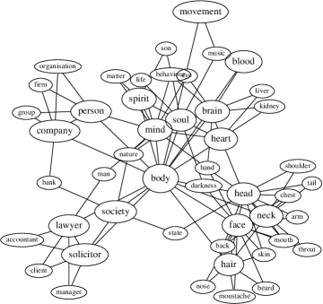
Figure 1: Local graph around body

The word graph has this very simple interpretation: Words which are directly linked are semantically close. This graph consists of $88,900$ nodes (word types) and $551,745$ edges. We ignore the order in which two words co-occur in a coordination, the edges in our graph are not given any direction. To reduce noise, we keep only those links in the graph which appear in a triangle, since the links within a triangle confirm each other’s significance. This results in a reduced word graph consisting of $48,727$ nodes and $505,412$ edges.

3 Graph curvature and quantifying semantic ambiguity

Our approach to assessing ambiguity is similar to the one proposed by ?), in that our measure also quantifies ambiguity based on the semantic cohesiveness of the target word’s neighborhood. Words with a very tightly-knit neighborhood are assigned smaller ambiguity scores than words whose neighborhood is rather fuzzy.

We measure the semantic cohesiveness of a word’s neighborhood (and as a result ambiguity) as the curvature of the word in the graph. Curvature is a property of nodes in a graph which quantifies the interconnectedness of a node’s neighbors. The curvature $\mbox{curv}(w)$ of a node $w$ is defined by:

$$\mbox{curv}({w})=\frac{\mbox{\#(triangles $w$ participates in)}}{\mbox{\#(triangles $w$ could participate in)}}$$

Curvature is the fraction of existing links among a node’s neighbors out of all possible links between neighbors. It assumes values between $0$ and $1$. A value of $0$ occurs if there is no link between any of the node’s neighbors (i.e. the neighbors are maximally disconnected), and a node has a curvature of $1$ if all its neighbors are linked (i.e. its neighborhood is maximally connected). Fig. 2 shows nodes of low, medium and high curvature respectively.

Figure 2: Left: $\mbox{curv}(v_{0})=0$, Right: $\mbox{curv}(v_{0})=0.3$, Bottom: $\mbox{curv}(v_{0})=1$.

Curvature measures whether neighbors of a word are neighbors of each other. Very specific unambiguous words have high curvature, because they usually live in small, semantically very cohesive communities in which many pairs of nodes have mutual neighbors. These communities thus contain a high density of triangles. Examples for tight word communities are the days of the week, the world religions, Greek gods, chemical elements, English counties, the planets, the members of a rock band, etc. Ambiguous words, on the other hand, are linked to members of different communities (corresponding to the different meanings of $w$) which do not know each other. An ambiguous word’s neighborhood thus has a low density of triangles which results in a low curvature value.

In information theory, it is common to use the negative logarithm of relative word frequency to measure a word’s information content ($\mbox{info}(w)=-\mbox{log}(\mbox{rf}(w))$). The intuition is that very frequent words tend to be very general and uninformative, and that very infrequent words tend to be more specific. Among the most frequent words in our model are countries, which according to ${\mbox{info}(\cdot)}$ would be wrongly categorized as very uninformative, ambiguous words.

Fig. 3 is a plot of curvature against frequency in our model. The countries among the nodes are indicated by black stars. Very clearly, the curvatures of the countries are considerably higher than the average curvature of words with similar frequency in the model, suggesting that, despite their high frequency, they are all very informative, i.e. unambiguous. The outlier in the lower left corner of the plot is monaco which may not seem ambiguous, but which has several different meanings in the BNC: country, city, 14th century painter and 20th century tenor (cf. Fig. 4).

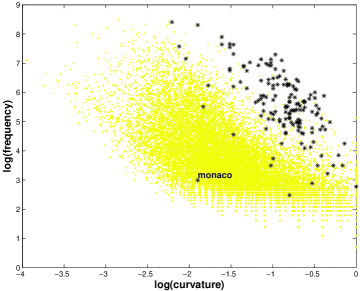
Figure 3: Curvature vs. model frequency

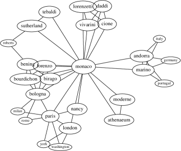
Figure 4: Local graph around monaco

To check how well curvature is suited for detecting and assessing ambiguity, we take all words in our model which are listed in WordNet and check how strongly curvature and the number of WordNet senses are related. Since the relationship does not have to be linear, we replace curvature and number of WordNet senses by their ranks before computing the Pearson correlation coefficient. We also wanted to see whether and to which degree curvature better reflects ambiguity than a word’s frequency in the model or its degree (the number of links attached to a node) in the graph. Table 1 lists the mutual Pearson correlations between any two quantities out of model frequency, degree, curvature and number of WordNet senses. Our analysis shows that with a negative correlation of $-0.538$, curvature is more strongly related to the number of WordNet senses and thus a better measure of ambiguity than model frequency or degree.

Table 1: Rank correlations between any two out of number of WordNet senses, word frequency in the model, degree and curvature.

	senses	freq	deg	curv
senses	1.000	0.475	0.480	-0.538
freq		1.000	0.963	-0.865
deg			1.000	-0.884
curv				1.000

4 Inducing classes of similar words

A semantic category (also referred to as a semantic field) is a grouping of vocabulary within a language, organizing words which are interrelated and define each other in various ways. The acquisition of semantic categories from text has been addressed in several different ways: Work in this direction can be found in (?), ?), ?), ?)).

Word clustering techniques differ in the way they assign words to clusters, either allowing words to belong to several clusters (soft clustering), or assigning words to one and only one cluster (hard clustering). A problem of hard clustering techniques is that each word is coerced into a single cluster irrespective of whether it is closely associated with other clusters, too.

Semantic categories overlap considerably, but hard clustering produces mutually exclusive clusters and forces ambiguous words to associate with a single cluster only. We therefore concentrate on soft clustering.

4.1 Graph clustering

In the following, we describe two approaches to soft clustering of words in our graph.

Curvature clustering: In our word graph, ambiguous words function as bridges between different word communities, e.g. cancer is the meeting point of the animal community, the set of lethal diseases and the signs of the zodiac. By removing these “semantic hubs”, the graph decomposes into small pieces corresponding to cohesive semantic categories. In detail, the method for extracting clusters of similar words is the following: 1. Compute the curvature of each node in the graph. 2. Remove all nodes whose curvature falls below a certain threshold ($0.5$). 3. The resulting connected components constitute clusters of semantically similar words.

Application of this algorithm to our word graph results in 700 clusters of size $\geq 2$. The resulting clustering covers $2,306$ of the nouns in our model with $21,218$ of the nodes not making the $0.5$ curvature threshold and $25,203$ isolated nodes.

This method produces a hard clustering of the high curvature words. Since high curvature words have a well-defined meaning, we expect a hard clustering approach to detect the (unique) semantic category each of these words belongs to.

Curvature clustering in this form cannot give information on the semantically fuzzy low curvature words. Therefore, we augment each of the clusters with the nodes attached to it. Table 2 lists some of the enriched clusters. The original cluster (the core of the extended cluster) is printed in bold font, cluster neighbors which did not pass the curvature threshold are highlighted in italics, and neighbors which were isolated in the initial clustering are printed in normal font. Often, the core words of high curvature are quite specific and unambiguous, suggesting that high curvature is a desirable property for ‘seed words’ (as in [Roark and Charniak, 1998]) used for this purpose. By extending the core clusters to their neighbors, coverage could be increased to $7,532$ nodes in the graph.

Table 2: Clusters resulting from the curvature approach

applewood fruitwood cherry ivory pine oak
jainism sikhism vaisnavism islam buddhism hinduism christianity judaism
horseflies lacewings butterfly mosquito beetle centipedes ladybird bird moth
freestyle backstroke butterfly race medley
printmaker ceramicist sculptor painter draughtsman artist
pomelo papaya banana potato pineapple mango peach palm pear parsnip
poliomyelitis tetanus tb kinase cough polio diphtheria malaria disease tuberculosis pertussis anthrax
thiamin niacin riboflavin fibre protein iron calcium
oratorio cantata concert baroque opera aria motet play
morphine methadone chloroform heroin caffeine length phosphate cocaine lsd librium metabolite
stepsister stepbrother friend father sister stepmother brother
insectivores artiodactyls ungulates mammal herbivore individual carnivore rodent horse order fruit
cosine tangent area sine torsion factor

Markov Clustering: A very intuitive graph clustering algorithm is Markov Clustering (http://micans.org/mcl/) developed by ?). Markov Clustering (MCL) partitions a graph via simulation of random walks. The idea is that random walks on a graph are likely to get stuck within dense subgraphs rather than shuttle between dense subgraphs via sparse connections.

MCL computes a hard clustering. The nodes in the graph are divided into non-overlapping clusters. Thus, nodes between dense regions will appear in a single cluster only, although they are attracted by different communities. Inspired by Schütze’s method [Schütze, 1998] we next replace clustering of word strings by clustering of word contexts.

4.2 Clustering the link graph

We consider pairs of words which we linked earlier, as word contexts. For example, organ occurs in contexts (organ, piano), (organ, harpsichord), (organ, tissue) and (organ, muscle). In contrast to the semantic “fuzziness” of organ, each of its contexts has a sharp-cut meaning and refers to exactly one of the senses of organ. By clustering word contexts as opposed to clustering the words themselves, a word’s different meanings can be distributed across different clusters which are then interpreted as word senses. E.g. we can assign (organ, piano) and (organ, harpsichord) to one context cluster, and (organ, tissue) and (organ, muscle) to another different context cluster.

In the setting of Sect. 2, words correspond to nodes in the word graph and word contexts coincide with the graph’s edges (with each edge being a context of the two nodes it joins). We now consider edges as the fundamental nodes of the link graph $G^{\prime}$, and define the edges of $G^{\prime}$ as follows: We construct the word graph’s associated link graph, $G^{\prime}$, by (see Fig.  7):   1. Introducing a node $n_{l}$ for each link $l$ in the original graph $G$.   2. Connecting any two nodes $n_{l_{1}}$ and $n_{l_{2}}$ in $G^{\prime}$ if $l_{1}$ and $l_{2}$ co-occurred in a triangle in $G$.

The two component words $u$ and $v$ of a context $l=(u,v)$ disambiguate each other, e.g. in the (organ, harpsichord) context, both organ and harpsichord are instruments, since this is the intersection of all the possible meanings of organ and all the possible meanings of harpsichord. The nodes $n_{l}$ introduced in step 1 therefore have a much narrower meaning than the nodes in $G$.

The links of a triangle in $G$ constitute mutually overlapping word contexts. We therefore expect the links in such a context triangle to have the same “topic”, and the nodes at the corners of the triangle to have the same meaning. This means, step 2 connects two nodes $n_{l_{1}}$ and $n_{l_{2}}$ if the corresponding contexts $l_{1}$ and $l_{2}$ are semantically similar.

Fig. 5 shows the local word graph around organ. Its associated link graph is illustrated in Fig. 6 (only those connected components containing organ with more than one node are displayed). Note that in the link graph, neighbors corresponding to different senses of organ are no longer linked.

Instead of clustering words by partitioning the original graph $G$, we cluster word contexts by partitioning $G$’s associated link graph $G^{\prime}$. The nodes $n_{l}$ in $G^{\prime}$ are built with contextual information, and thus typically have a clear-cut meaning. With little (if any) ambiguity left in the link graph, a hard clustering algorithm, such as MCL, is fit for dividing the contexts into (non-overlapping) similarity classes. In detail, our algorithm is: 1) Start with the original graph $G$. 2) Construct the associated link graph $G^{\prime}$. 3) Apply Markov Clustering to $G^{\prime}$. 4) Merge clusters whose overlap in information exceeds a certain threshold.

The clustering resulting from step 3 is too fine-grained. Several of the context clusters describe the same “topic”. We collapse these multiple clusters via another application of MCL, this time applied to a graph of context clusters which are linked if their shared information content (the negative logarithm of the probability of the words they have in common) exceeds $50\%$ of the information contained in the smaller of the two clusters. Step 4 reduced the $12,786$ clusters resulting from step 3 to a total of $5,849$ clusters.

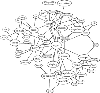
Figure 5: Local word graph around organ

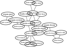
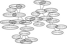
Figure 6: Its associated link graph

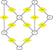
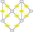
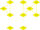
Figure 7: From $G$ to $G^{\prime}$. The original graph, new nodes $n_{l}$ , new links, the graph $G^{\prime}$.

5 Comparative evaluation for lexical acquisition

One of the principal uses of word clustering techniques is to supply missing lexical information. For example, the hypernyms of a word $a$ can often be inferred from the hypernyms of its neighbors $b_{1},\ldots,b_{n}$. This property was used by [Hearst and Schütze, 1993] and [Widdows, 2003] to map unknown words into the WordNet taxonomy. The accuracy of such methods depends on the taxonomy in question, the method used to obtain the neighbors $b_{1},\ldots,b_{n}$, and the specificity of the result desired.

From the subset of nouns in our test graph known to WordNet, we randomly picked a set of 1,200 test words consisting of 600 proper nouns and 600 common nouns. Each of these two subsets is further divided into 3 frequency categories (top (500-1000), mid (250-1000), low (below 250)) which consist of 200 words each.

Pretending that we don’t know the test words, we test how well we do in re-mapping them into WordNet. For each of the test words $t$, we look up which clusters it appears in and keep its most similar cluster $c_{\max}$. Similarity between words and clusters is computed using cosine similarity between their vector representations in a vector space model [Deerwester et al., 1990].

We then assign a sense label to $c_{\max}$ using the sense-labeling algorithm proposed in [Widdows, 2003] which treats any hypernym of any of the cluster members as a potential cluster label. Potential cluster labels are rated based on two competing criteria: $\bullet$ The more cluster members a label subsumes, the better (favoring more general labels). $\bullet$ The more informative the label, the better (favoring more specific labels). Since including the test word $t$ in the sense-labeling process would be using information about $t$ which we are not given in a real lexical acquisition situation, we disregard both, the test word and the cluster members which are morphologically related to the test word.

The labeling algorithm outputs a cluster’s top five labels together with a score assessing their adequacy. We compare each of these labels with each of the test word’s ancestors in WordNet, and, in case of a match, record the number of intervening levels between the test word and the label. E.g. the test word opera appears in the cluster (jazz, music, festival, sound, beat, reggae, soul, ballet, funk, country, orchestra, film, table, poetry). Table 3 shows the cluster labels and scores assigned by the class-labeling algorithm. Column match lists the number of intervening WordNet levels between opera and each of the labels.

If a test word $t$ is not covered by the clustering, we do a depth-first search on the original word graph starting at $t$ and moving along the strongest link until we reach a node $t^{\prime}$ covered by the clustering. We then pretend that $t$ belongs to the cluster(s) $t^{\prime}$ appears in.

Table 3: Labels assigned to the opera cluster

label	score	match
auditory communication	0.438	4
communication	0.076	5
abstraction	-0.265	8
relation	-0.500	7
social relation	-0.603	6

To summarize, evaluation consists of the following steps. For each test word $t$,  1. If $t$ doesn’t appear in any cluster, follow strongest links until you reach a word $t^{\prime}$ which is covered by the clustering and substitute $t$ with $t^{\prime}$.  2. Collect the clusters $t$ appears in.  3. Compute the similarity between $t$ and each of the clusters and keep only the cluster $c_{\max}$ which is most similar to $t$.  4. Compute a class label $l$ for $c_{\max}\setminus\{t\}$.  5. Check if (and how closely) $l$ corresponds to one of $t$’s WordNet senses.

Basis for comparison

We use the following simple sense-labeling method as basis for comparison. For each test word $t$, we find its nearest neighbor $n$ in the graph. For all the hypernyms of $t$ and $n$, we find their common subsumer $\mbox{cs}(t,n)$ which minimizes the average distance to $t$ and $n$. We are directly using taxonomic knowledge about our test word $t$ to find the optimal position in the WordNet tree where $t$ and $n$ should join. In a real lexical acquisition situation, of course, such information is not available. This method therefore forms a simplest upper bound on how well we could expect to do in mapping unknown words into the WordNet taxonomy.

Results

Table 6 summarizes the performance of the algorithms on the lexical acquisition task described above (similar results are obtained for proper nouns). For each test set and each method, row N lists the number (percentage) of test words which are not in WordNet. The number (percentage) of words which received a label not corresponding to any of its senses with any number of intervening WordNet levels is listed in row W. The rows $i=1..12$ contain the number of words which were assigned a correct label with $i$ or less intervening WordNet levels. For these rows, the percentages in parentheses are relative to the total number of words which were assigned a correct label.

Naturally, the baseline method, which is using (normally unknown) taxonomic information about the test word itself, performs best. Of all the methods, it has the fewest number of wrongly assigned labels (row W). An accuracy of $92\%$, resp. $99\%$ is reached at $\leq 5$ intervening WordNet levels.

6 Conclusions

Among the other three methods, Markov Clustering (MCL) of the link graph outperforms both MCL on the original graph and curvature clustering. The number of wrongly assigned labels is about half of those for curv and orig and the values in the 12 rows are consistently higher with an accuracy of over $85\%$ at $\leq 6$ WordNet levels. The link graph clustering therefore produces more accurate labels. In the top frequency category, MCL on the original graph has a slightly higher percentage of correctly assigned class labels for small numbers of intervening WordNet levels, but is soon overtaken by the link graph clustering. The lower values for the curvature clustering can be partly explained by its low coverage. $854$ of the $1,200$ test words were not covered by the curvature clustering and had to be traced to clusters using depth-first search in 1 to 46 steps (with $60\%$ ($80\%$) of the test words being at most $3$ ($6$) links apart from a cluster).

Judging by the classes in Table 2, we expect curvature clustering to do especially well in recognizing the meanings of words unknown to WordNet.

Table 4: Evaluation results for common nouns

	nn1_top
Not	2(0.01)	2(0.01)	2(0.01)	2(0.01)
Wrong	74(0.37)	32(0.16)	69(0.34)	14(0.07)
1	21(0.17)	23(0.14)	8(0.06)	38(0.21)
2	40(0.32)	47(0.28)	26(0.20)	62(0.34)
3	66(0.53)	79(0.48)	50(0.39)	84(0.46)
4	90(0.73)	106(0.64)	70(0.54)	99(0.54)
5	99(0.80)	128(0.77)	89(0.69)	183(0.99)
6	108(0.87)	143(0.86)	103(0.80)	183(0.99)
7	114(0.92)	153(0.92)	110(0.85)	183(0.99)
8	118(0.95)	161(0.97)	120(0.93)	184(1.00)
9	121(0.98)	164(0.99)	124(0.96)	184(1.00)
10	121(0.98)	164(0.99)	127(0.98)	184(1.00)
11	122(0.98)	166(1.00)	129(1.00)	184(1.00)
12	123(0.99)	166(1.00)	129(1.00)	184(1.00)
	nn1_mid
Not	0(0.00)	0(0.00)	0(0.00)	0(0.00)
Wrong	65(0.33)	38(0.19)	77(0.39)	25(0.12)
1	19(0.14)	17(0.11)	9(0.07)	33(0.19)
2	36(0.27)	45(0.28)	22(0.18)	62(0.35)
3	63(0.47)	74(0.46)	43(0.35)	80(0.46)
4	86(0.64)	105(0.65)	60(0.49)	90(0.51)
5	100(0.75)	127(0.79)	76(0.62)	174(0.99)
6	111(0.83)	139(0.86)	93(0.76)	174(0.99)
7	124(0.93)	150(0.93)	113(0.93)	174(0.99)
8	128(0.96)	156(0.97)	118(0.97)	174(0.99)
9	130(0.97)	158(0.98)	120(0.98)	174(0.99)
10	132(0.99)	159(0.99)	121(0.99)	174(0.99)
11	134(1.00)	161(1.00)	122(1.00)	174(0.99)
12	134(1.00)	161(1.00)	122(1.00)	174(0.99)
	nn1_low
Not	4(0.02)	4(0.02)	4(0.02)	4(0.02)
Wrong	65(0.33)	47(0.23)	82(0.41)	38(0.19)
1	17(0.13)	13(0.09)	6(0.05)	20(0.13)
2	31(0.24)	33(0.22)	14(0.12)	32(0.20)
3	43(0.33)	64(0.43)	26(0.23)	50(0.32)
4	69(0.53)	87(0.58)	52(0.46)	62(0.39)
5	93(0.71)	112(0.75)	68(0.60)	145(0.92)
6	102(0.78)	127(0.85)	75(0.66)	152(0.96)
7	116(0.89)	132(0.89)	93(0.82)	156(0.99)
8	120(0.92)	143(0.96)	97(0.85)	157(0.99)
9	125(0.95)	147(0.99)	104(0.91)	158(1.00)
10	129(0.98)	148(0.99)	109(0.96)	158(1.00)
11	130(0.99)	148(0.99)	111(0.97)	158(1.00)
12	131(1.00)	149(1.00)	114(1.00)	158(1.00)

We have shown that graphs can be learned directly from free text and used for ambiguity recognition and lexical acquisition. We introduced two new combinatoric techniques, graph curvature and link clustering, and evaluated their contribution as clustering methods for lexical acquisition. Link clustering produces particularly promising results when compared with information in the WordNet noun hierarchy. These results demonstrate that our combinatoric methods for analysing the geometry and topology of graphs improve language learning.

References

- Chartrand, 1985 G. Chartrand. 1985. Introductory Graph Theory. Dover.
- Deerwester et al., 1990 S. Deerwester, S. Dumais, G. Furnas, T. Landauer, and R. Harshman. 1990. Indexing by latent semantic analysis. Journal of the American Society for Information Science, 41(6):391–407.
- Dorow and Widdows, 2003 B. Dorow and D. Widdows. 2003. Discovering corpus-specific word-senses. In Proceedings of EACL, pages Conference Companion pp. 79–82, Budapest, Hungary, April.
- Eckmann and Moses, 2002 J.-P. Eckmann and E. Moses. 2002. Curvature of co-links uncovers hidden thematic layers in the world-wide web. In Proceedings of the Natl. Acad. Sci. USA, volume 99, pages 5825–5829.
- Hearst and Schütze, 1993 M. Hearst and H. Schütze. 1993. Customizing a lexicon to better suit a computational task. In ACL SIGLEX Workshop, Columbus, Ohio.
- Hearst, 1992 M. Hearst. 1992. Automatic acquisition of hyponyms from large text corpora. In COLING, Nantes, France.
- Pantel and Lin, 2002 P. Pantel and D. Lin. 2002. Discovering word senses from text. In Proceedings of ACM SIGKDD 2002, Edmonton, Canada.
- Pereira et al., 1993 F. Pereira, N. Tishby, and L. Lee. 1993. Distributional clustering of english words. In Proceedings of ACL, pages 183–190, Columbus, Ohio.
- Riloff and Shepherd, 1997 E. Riloff and J. Shepherd. 1997. A corpus-based approach for building semantic lexicons. In Proceedings of the Second Conference on Empirical Methods in NLP, pages 117–124. ACL, Somerset, New Jersey.
- Roark and Charniak, 1998 B. Roark and E. Charniak. 1998. Noun-phrase co-occurence statistics for semi-automatic semantic lexicon construction. In COLING-ACL, pages 1110–1116.
- Schütze, 1998 H. Schütze. 1998. Automatic word sense discrimination. Computational Linguistics, 24(1):97–124.
- Sigman and Cecchi, 2002 M. Sigman and G. Cecchi. 2002. The global organization of the wordnet lexicon. In Proceedings of the Natl. Acad. Sci. USA, volume 99, pages 1742–1747, February.
- Sproat and van Santen, 1998 R. Sproat and J. van Santen. 1998. Automatic ambiguity detection. In Proceedings of ICSLP 98, Sydney, Australia.
- van Dongen, 2000 S. van Dongen. 2000. Graph Clustering by Flow Simulation. Ph.D. thesis, University of Utrecht, May.
- Widdows and Dorow, 2002 D. Widdows and B. Dorow. 2002. A graph model for unsupervised lexical acquisition. In Proceedings of Coling, pages 1093–1099, Taipei, Taiwan, August.
- Widdows, 2003 D. Widdows. 2003. Unsupervised methods for developing taxonomies by combining syntactic and statistical information. HLT-NAACL, Edmonton, Canada.