Detrended fluctuation analysis as a statistical tool to monitor the climate

Abstract

Detrended fluctuation analysis is used to investigate power law relationship between the monthly averages of the maximum daily temperatures for different locations in the western US. On the map created by the power law exponents, we can distinguish different geographical regions with different power law exponents. When the power law exponents obtained from the detrended fluctuation analysis are plotted versus the standard deviation of the temperature fluctuations, we observe different data points belonging to the different climates, hence indicating that by observing the long-time trends in the fluctuations of temperature we can distinguish between different climates.

1 INTRODUCTION

Recent advances has shown us that we can use scaling arguments to analyze climatic data [1, 2, 3, 4, 5, 6, 7, 8, 9, 10, 11, 12, 13, 14, 15, 16, 17, 18, 19]. The ongoing discussion focuses on whether we can obtain a correlation between the scaling exponents obtained from these analyses and the geographic location of the weather stations [1, 4, 19, 20, 21].

Determining the weather is a rather simple issue. A cold day is usually followed by a cold day, and a warm day is usually followed by a warm day. On a larger scale, a colder week is usually followed by a warmer week which corresponds to the average duration of the general weather regimes. But as the longer timescales are governed by different processes like the circulation patterns and sometimes even influenced by trends like global warming, defining long-term correlations becomes more difficult.

In order to separate the trends and the correlations we need to eliminate the trends in our temperature data. Several methods are used effectively for this purpose: rescaled range analysis (R/S) [14, 15, 22, 23], wavelet techniques (WT) [12, 24] and detrended fluctuation analysis (DFA) [13, 25].

Analysis of the temperature fluctuations over a period of decades in different places of the globe has already showed the effectiveness of the application of detrended fluctuation analysis to characterize the persistence of weather and climate regimes. DFA and WT have been applied to study temperature and precipitation correlations in different climatic zone on the continents and also in the sea surface temperature of the oceans. The recent results show that the temperatures are long range power law correlated. The long-term persistence of the temperatures can be characterized by an auto-correlation function $C(n)$ of temperature variations where $n$ is the time between the observations. The auto-correlation function decays as $C(n)\sim n^{-\gamma}$. Even though there is some disagreement on the value of the exponent $\gamma$, the fact that the persistence of the temperatures can be characterized by this auto-correlation function is firmly established. Different groups have used R/S, DFA and WT analysis and have shown that this exponent $\gamma$ has roughly the same value $\gamma\simeq 0.7$ for the continental stations [4, 7, 10, 13, 14, 15, 16, 17]. The exponent $\gamma$ is found to be roughly 0.4 for island stations [4, 7] and sea surface temperature on the oceans [6, 7]. This method has also been applied to the temperature predictions of coupled atmosphere-ocean general circulation models [1, 8, 19, 21, 26] but there is disagreement on the actual value of the exponent $\gamma$. On one side it is argued that the exponent does not change with the distance from the oceans [1, 4] and is roughly $\gamma\simeq 0.7$. On the other side it is said that the scaling exponent is roughly 1 over the oceans, roughly 0.5 over the inner continents and about 0.65 in transition regions [21].

Previous work in this area also shows that there is a slight variation in the scaling exponent between the low-elevation, mountain, continental and maritime stations [16, 17]. Even though these variations are between $\gamma\simeq 0.5$ and $\gamma\simeq 0.7$ the fact that they show a correlation with location and elevation indicates that a relationship between the statistical nature of the temperature fluctuations and the climate can be established.

The work presented in this paper focuses on the statistical aspect of the temperature data and tries to establish a method to analyze temperature records in such a way as to reveal long term trends in the climate with the hope to help the models created to measure climate change.

2 METHOD

To remove the seasonal trends that are known to exist in the daily temperature data we need to determine the mean temperature for each day over all the years in the time series. We then calculate the fluctuation of the daily temperature from the mean daily temperature,

$$\Delta T_{i}=T_{i}-<T_{i}>$$ (1)

where $<T_{i}>$ is the mean daily maximum temperature. Similarly we can also use the mean daily average temperature or the mean daily minimum temperature, and the use of average or minimum temperature instead of maximum temperatures does not change the outcome of the analysis [17]. To remove the remaining linear trends in the data (the average temperature for some years can be higher or lower than the average temperature of the time series for that location as a result of long-term atmospheric processes), we applied Detrended Fluctuation Analysis (DFA) method [25], which is used to remove trends in the data to allow investigation of long-term correlations in the data.

The noise and the nonstationarity in the temperature data usually hinders a reliable and direct calculation of the autocorrelation function $C(n)$, instead we calculate a running sum of the temperature fluctuations,

$$y(m)=\sum_{i=1}^{n}\Delta T_{i}$$ (2)

where $m=1,...,n$. Next, the time series of the $y(m)$ is divided into nonoverlapping intervals of equal length $n$. In each interval, we fit $y(m)$ to a straight line, $x(m)=km+d$ for each segment and calculate the detrended square variability $F^{2}(n)$ as

$$F^{2}(n)=<\frac{1}{n}\sum_{m=kn+1}^{(k+1)n}(y(m)-x(m))^{2}>$$ (3)

with

$$k=0,1,2,...,(\frac{N}{n}-1).$$ (4)

If the temperature fluctuations were uncorrelated (white noise) we would expect

$$F(n)\sim n^{\alpha}$$ (5)

where $\alpha=\frac{1}{2}$. If $\alpha>\frac{1}{2}$, we would expect long-range power law correlations in the data for the range of values considered. Figure 1 shows an example of such an analysis method for a sample station, Cheyenne WSFO, WY. The data follows a straight line with slope $\alpha=0.58\pm 0.01$. Even though there is some scatter in the data after a period of 10 years, the scatter in the data is still within the error bars of the analysis. This scatter is caused by the fact that the average in the detrended square variability $F^{2}(n)$ has been taken over larger and larger values of $n$, resulting in poor statistics. The dataset consists of 107 years of monthly temperature data between the years 1888-1994.

Figure 1: The power law relationship between the time period and the detrended square variability. The data is for a sample station, Cheyenne WSFO, WY with slope $\alpha=0.63\pm 0.01$.

The main problem when we want to adopt this analysis to climate is the absence of high quality long-term daily temperature data. When we need to look at the short term fluctuations in daily temperatures, we must obtain reliable data, however if our aim is long-term behavior of temperature data we can also use monthly averages instead of daily averages. It has been shown that for the time domain longer than 60 days, both the daily and monthly temperature data give us the same scaling exponent [16, 17]. As our analysis for daily and monthly data at all the sampled locations also agrees for long time scales ($n>60days$) the results presented in the paper have been obtained from the analysis of monthly averages.

In the present work we have investigated temperature fluctuations for 384 weather stations in the Western US. The data has been obtained from the U.S. Historical Climatology Network [27]. From the available data we have chosen the stations with the longest records. We did not include in our analysis datasets with data shorter than 75 years, and the longest dataset we had was 110 years at several locations in the dataset (all ending in 1994).

Previously it has been observed that power law exponents obtained from DFA of temperature fluctuations stay between 0.55 and 0.70 [1, 4, 8, 12, 13]. Figure 2 gives a summary of the scaling exponents obtained from the 384 stations in the Western US. As we can see from this figure, consistent with the earlier observations, we obtain scaling exponents in the range of 0.50 to 0.74. The average for all the dataset investigated comes out to be $\bar{\alpha}=0.61\pm 0.04$.

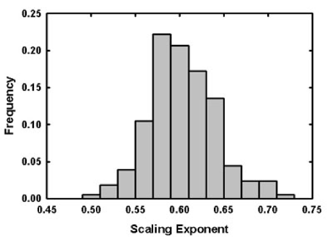
Figure 2: The histogram of the scaling exponents is shown. The average from 384 stations gives a scaling exponent of $\bar{\alpha}=0.61\pm 0.04$.

Figure 3 shows a map of all the power law exponents for all the stations. This map has been generated using the data using a running average method to generate a grid of 30 x 30 regions with the data we have. A simple observation about the power law exponents is even though the power law exponents crowd around the mean value, their special distribution is not uniform. From the map we can simply distinguish a few regions: Western part of Washington and Oregon, Montana region, Inland California, Utah and New Mexico. Table 1 gives the power law exponents for these regions. This table is sufficient to divide the western US into two different regions, one with high power law exponent $\bar{\alpha}=0.64\pm 0.04$ and one with lower power law exponent $\bar{\alpha}=0.59\pm 0.01$.

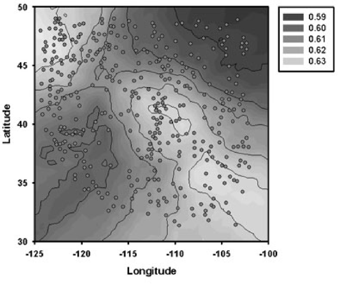
Figure 3: The map of the power law exponents for the western US. The stations are presented by circles in the data. The interpolation has been done using the running average method.

However, such a division is not sufficient because of two main reasons:

• Western Oregon and New Mexico are both categorized as high power law exponent regions. But when we look at the climate of these regions we see very different characteristics, western Oregon stations predominantly being Humid Subtropical Mediterranean ($83\%$ of the stations in this region) whereas New Mexico is mostly dry/arid (cool) mid latitude desert ($88\%$ of the stations in this region).

• New Mexico and Coastal California are categorized as high and low power law exponent regions respectively. But when we look at the climate of these regions we see very similar characteristics, both regional stations mostly being dry/arid (cool) mid latitude desert (New Mexico - $88\%$, coastal California - $70\%$ of the stations).

However a striking result can be observed if we plot the standard deviation of the temperature fluctuations versus the power law exponent observed from these stations. Figure 4 gives a summary of the power law exponents for the six regions mentioned in Table 1, Western Washington and Oregon, New Mexico, Utah, Coastal California, Inland California and Western Nevada, and Montana, versus the standard deviation of the temperature fluctuations, respectively. In this figure we can clearly identify that, with the aid of the standard deviation of temperature fluctuations, the scaling exponents can be used to distinguish between different climates, and perhaps bring some refinements to the already existing classification [28].

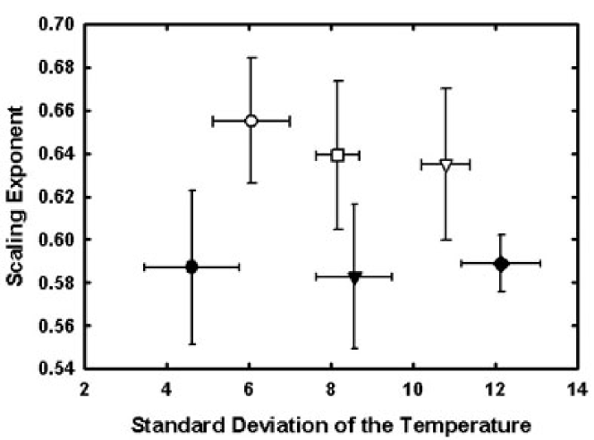
Figure 4: The scaling exponents plotted against the standard deviation of the temperature fluctuations for Western Washington and Oregon (empty circles), New Mexico (empty squares), Utah (empty triangles), Coastal California (full circles), Inland California and Western Nevada (full triangles), and Montana (full diamonds).

Table 1: Power law exponents for different regions of Western United States.

Region:	Power Law Exponent:
Western Oregon and Washington	$0.66\pm 0.03$
Utah and Western Colorado	$0.64\pm 0.03$
New Mexico, Oklahoma panhandle, Southern Colorado	$0.64\pm 0.03$
Inland California and Western Nevada	$0.58\pm 0.03$
Montana and Western North Dakota	$0.59\pm 0.01$
Coastal California	$0.59\pm 0.03$

3 DISCUSSION

We have investigated the power law behavior of the temperature fluctuations to gain more insight to a statistical description of different climate types. The main question in this regard that would come to mind is why not simply use the regular way of measuring temperature, pan evaporation and precipitation to determine the climate type for a region. Most certainly we do not need a sharper method than using the meteorological data for the present climate in our world, however for two major reasons we would need a statistical method to describe the climates.

When we look at the climatic data and how it has changed in the past, we need a method to analyze paleoclimatic data to reveal structure of timescales not only of the order of decades but millions of years. But the difficulty shows itself as the paleoclimatic data come from a number of different data sources and they have different units. But only one thing is common to all of this data, and that is the fact that all of this data is in terms of a time series of amplitudes. Our results suggest that on the basis of power law scaling of the temperature fluctuations of the maximum daily temperatures we can distinguish between different climates. The real challenge comes when we try expand this analysis into the past, as to our knowledge, no reliable monthly data exists beyond 218 years [12]. However, previous work where authors have established long-range power law behavior using rescaled-range analysis [29, 30] gives us hope about expanding the use of the method we have developed.

When we use global climate models to extrapolate the climate changes into the future, the method of detrended fluctuation analysis proves to be a powerful tool [8, 19]. When the length scale and the future time scale of application of these climate models improves the present work may help to fill in the voids in the models by providing information on how the climate would be like.

References

References

- [1] A. Bunde, J. Eichner, R. Govindan, S. Havlin, E. Koscielny-Bunde, D. Rybski, D. Vjushin, Preprint, physics/0208019 (2003).
- [2] J. W. Kantelhardt, D. Rybski, S. Zschiegner, P. Braun, E. Koscielny-Bunde, V. Livina, S. Havlin, A. Bunde, Physica A 330, 240 (2003).
- [3] E. Koscielny-Bunde, J. W. Kantelhardt, P. Braun, A. Bunde, S. Havlin, Preprint, physics/030578 (2003).
- [4] J. Eichner, E. Koscielny-Bunde, A. Bunde, S. Havlin, H. J. Schnellnhuber, Phys. Rev. E 68, 046133 (2003).
- [5] V. Livina, Y. Ashkenazy, P. Braun, R. A. Monetti, A. Bunde, S. Havlin, Phys. Rev. E 67, 042101 (2003).
- [6] R. A. Monetti, S. Havlin, A. Bunde, Physica A 320, 581 (2003).
- [7] A. Bunde, S. Havlin, Physica A 314, 15 (2002).
- [8] R. Govindan, D. Vjushin, A. Bunde, S. Brenner, Y. Ashkenazy, S. Havlin, H. J. Schnellnhuber, Phys. Rev. Lett. 89, 028501 (2002).
- [9] D. Vjushin, R. Govindan, S. Brenner, A. Bunde, S. Brenner, S. Havlin, H. J. Schnellnhuber, J. Phys.: Cond. Matt. 14, 2275 (2002).
- [10] J. W. Kantelhardt, E. Koscielny-Bunde, H. H. A. Rego, S. Havlin, A. Bunde, Physica A 295, 441 (2001).
- [11] R. Govindan, D. Vjushin, S. Brenner, A. Bunde, S. Havlin, H. J. Schnellnhuber, Physica A 294, 239 (2001).
- [12] E. Koscielny-Bunde, A. Bunde, S. Havlin, H. E. Roman, Y. Goldreich, H. J. Schnellnhuber, Phys. Rev. Lett. 81, 729 (1998).
- [13] E. Koscielny-Bunde, A. Bunde, S. Havlin, Y. Goldreich, Physica A 231, 231 (1996).
- [14] L. Bodri, Theoretical and Applied Climatology 51, 51 (1995).
- [15] L. Bodri, Theoretical and Applied Climatology 49, 53 (1994).
- [16] R. O. Weber, P. Talkner, J. Geophys. Res. Atmos. 106, 20131 (2001).
- [17] P. Talkner, R. O. Weber, Phys. Rev. E 62, 150 (2000).
- [18] R. O. Weber, P. Talkner, G. Stefanicki, Geophys. Res. Lett. 21, 673 (1994).
- [19] K. Fraedrich, R. Blender, Phys. Rev. Lett. 90, 108501 (2003).
- [20] A. Bunde, J. F. Eichner, S. Havlin, E. Koscielny-Bunde, H. J. Schnellnhuber, D. Vjushin, Phys. Rev. Lett. 92, 039801 (2004).
- [21] K. Fraedrich, R. Blender, Phys. Rev. Lett. 92, 039802 (2004).
- [22] B. B. Mandelbrot, J. R. Wallis, Water Resources Research 5, 321 (1969).
- [23] B. B. Mandelbrot, J. R. Wallis, Water Resources Research 5, 967 (1969).
- [24] A. Arneodo, E. Bacry, P. V. Graves, J. F. Muzy, Phys. Rev. Lett. 74, 3293 (1995).
- [25] C. K. Peng, S. V. Buldyrev, S. Havlin, M. Simmons, H. E. Stanley, A. L. Goldberger, Phys. Rev. E 49, 1685 (1994).
- [26] R. Blender, K. Fraedrich, Geophys. Res. Lett. 30, 1769 (2003).
- [27] U.S. Hist. Climat. Network, http:// cdiac.esd.ornl.gov/ epubs/ ndp019/ statemax.html.
- [28] W. Koeppen, Geographischen Zeitschrift 9, 593 (1900).
- [29] R. H. Fluegeman Jr., R. S. Snow, Pageoph. 131, 307 (1989).
- [30] Y. Wang, M. E. Evans, T. C. Xu, N. Rutter, Z. Ding, X. M. Liu, Can. J. Earth Sci. 29, 296 (1992).