Modularity from Fluctuations in Random Graphs and Complex Networks

Abstract

The mechanisms by which modularity emerges in complex networks are not well understood but recent reports have suggested that modularity may arise from evolutionary selection. We show that finding the modularity of a network is analogous to finding the ground-state energy of a spin system. Moreover, we demonstrate that, due to fluctuations, stochastic network models give rise to modular networks. Specifically, we show both numerically and analytically that random graphs and scale-free networks have modularity. We argue that this fact must be taken into consideration to define statistically-significant modularity in complex networks.

Statistical, mathematical, and model-based analysis of complex networks have recently uncovered interesting unifying patterns in networks from seemingly unrelated disciplines Watts and Strogatz (1998); Barabási and Albert (1999); Amaral et al. (2000); Albert and Barabási (2002); Dorogovtsev and Mendes (2002). In spite of these advances, many properties of complex networks remain elusive, a prominent one being modularity Girvan and Newman (2002); Newman and Girvan (2004). For example, it is a matter of common experience that social networks have communities of highly interconnected nodes that are poorly connected to nodes in other communities. Such modular structures have been reported not only in social networks Girvan and Newman (2002); Guimerà et al. (2003); Newman and Girvan (2004), but also in biochemical networks Hartwell et al. (1999), food webs Pimm (1979), and the Internet Eriksen et al. (2003). It is widely believed that the modular structure of complex networks plays a critical role in their functionality Hartwell et al. (1999). There is therefore a clear need to develop algorithms to identify modules accurately Girvan and Newman (2002); Newman and Girvan (2004); Eriksen et al. (2003); Newman (2003); Radicchi et al. (2004).

More fundamentally, the mechanisms by which modularity emerges in complex networks are not well understood. In biological networks—both biochemical and ecological—researchers have suggested that modularity increases robustness, flexibility, and stability Hartwell et al. (1999); Pimm (1979). Similarly, in engineered networks, it has been suggested that modularity is effective to achieve adaptability in rapidly changing environments Alon (2003). It may therefore seem that evolutionary pressures make networks modular, implying that any successful model of complex networks should take into account external factors that enhance modularity. Recently, however, Solé and Fernández have pointed out that models without any external pressure are able to give rise to modular networks Solé and Fernández (2003).

In this Letter, we show that Erdös-Rényi (ER) random graphs, in which any pair of nodes is connected with probability $p$ Bollobas (2001), have a high modularity. We show numerically and analytically that this high modularity is due to fluctuations in the establishment of links, which are magnified by the large number of ways in which a network can be partitioned into modules. Furthermore, we show that one obtains similar results when considering scale-free networks Barabási and Albert (1999). We conclude by discussing how these results should be taken into consideration to define statistically significant modularity in complex networks.

Following the first quantitative definition of modularity Newman and Girvan (2004); Newman (2003), several groups have proposed heuristic algorithms to detect modules in complex networks. For a given partition of the nodes of a network into modules, the modularity $\mathcal{M}$ of this partition is defined as Newman and Girvan (2004)

$$\mathcal{M}\equiv\sum_{s=1}^{r}\left[\frac{l_{s}}{L}-\left(\frac{d_{s}}{2L}\right)^{2}\right]\,,$$ (1)

where $r$ is the number of modules, $L$ is the number of links in the network, $l_{s}$ is the number of links between nodes in module $s$, and $d_{s}$ is the sum of the degrees of the nodes in module $s$. This definition of modularity implies that $\mathcal{M}\leq 1$ and that $\mathcal{M}=0$ for a random partition of the nodes Newman and Girvan (2004). We define the modularity $M$ of a network as the largest modularity of all possible partitions of the network $M=\max\{\mathcal{M}\}$.

The problem of finding the modularity of a network with $S$ nodes is therefore analogous to the standard statistical mechanics problem of finding the ground-state energy of the Hamiltonian $\mathcal{H}=-L\mathcal{M}$. Specifically, one can map the network into a spin system by defining the variables $s_{i}\in\{1,2,\dots,S\}$ as the module to which node $i$ belongs and the couplings $J_{ij}$ as being 1 if nodes $i$ and $j$ are connected in the network and 0 otherwise. Then, from Eq. (1), one can demonstrate that

$$\mathcal{H}= - \sum_{i,j}^{S}\frac{J_{ij}}{2}\;\delta_{s_{i}s_{j}}$$

$$+ \sum_{i,j,k,l}^{S}\left[\frac{J_{ij}J_{kl}}{16L}\left(\delta_{s_{i}s_{j}s_{k}s_{l}}+2\delta_{s_{i}s_{j}s_{k}}+\delta_{s_{i}s_{k}}\right)\right].$$

This Hamiltonian corresponds to an $S$-state Potts model with both ferromagnetic and anti-ferromagnetic terms, and two-, three-, and four-spin interactions. Therefore, it seems difficult to apply methods used in problems that are similar but formally simpler, like the graph coloring problem Mulet et al. (2002). Rather, we propose here a heuristic estimation of the modularity for a number of interesting graph models, namely low-dimensional regular lattices, ER random graphs Bollobas (2001) and scale-free networks Barabási and Albert (1999).

Low-dimensional regular lattices— Consider a one-dimensional lattice with $S$ nodes, each one connected to its two neighbors . This case is particularly simple because the modules comprise only contiguous nodes and, therefore, the number of between-module links equals the number $r$ of modules. Assuming that all modules have approximately the same size $n=S/r$, the modularity of a partition with $r$ modules is

$$\mathcal{M}_{1D}(S;r)=\frac{S-r}{S}-\frac{1}{r}\,,$$ (3)

where we have used the fact that the number $L$ of links is $L\approx S$. Under these assumptions, the problem of finding the modularity of a regular one-dimensional lattice is reduced to finding the optimal number $r^{*}$ of modules, that is, the number of modules that yields the maximum modularity. One can show that $r^{*}(S)=\sqrt{S}$, and the modularity is

$$M_{1D}(S)=1-\frac{2}{\sqrt{S}}\,.$$ (4)

Note that the only assumption in the calculation is that all modules have approximately the same number of nodes. Numerical results confirm that this is a sensible assumption.

One can generalize this result to one-dimensional lattices in which each node is connected to $z$ nodes on the left and $z$ on the right. In this case, the leading contributions to the modularity are

$$M_{1D}(S,z)=1-\sqrt{\frac{2(z+1)}{S}}\;.$$ (5)

Similarly, one can calculate the modularity of $d$-dimensional cubic lattices in which each node is connected to $2z$ nodes in each one of the $d$ directions, to obtain that Guimerà et al. (2004)

$$M_{dD}(S,z)=1-(d+1)\left(\frac{z+1}{2d}\right)^{\frac{d}{d+1}}\frac{1}{S^{\frac{1}{d+1}}}\;.$$ (6)

Random graphs— In ER random graphs Bollobas (2001), each pair of nodes is connected with probability $p$. As for $d$-dimensional lattices, we assume that the partition of the network with highest modularity consists of $r$ modules with approximately the same number of nodes $n=S/r$, the same number of within-module links $k_{i}$, and the same number of links $k_{o}$ to other modules. In the $S\gg 1$ limit, we can assume that the total number of links is $S^{2}p/2$ and, therefore, $k_{i}$ and $k_{o}$ are related by

$$k_{o}(S,p;r,k_{i})=\frac{S^{2}p}{r}-2k_{i}.$$ (7)

Hence, for $S\gg 1$, the modularity of such a partition is simply

$$\mathcal{M}_{ER}(S,p;r,k_{i})=\frac{2rk_{i}}{S^{2}p}-\frac{1}{r}\,.$$ (8)

Under these assumptions, the problem of finding the modularity of a random graph is reduced to finding a partition of the graph with the following properties: (i) The partition consists of $r$ equal modules, each one with $k_{i}$ within-module links; (ii) The partition typically exists in a random graph; and (iii) The partition yields the maximum modularity relative to the other partitions that typically exist.

In a random graph with $S$ nodes and linking probability $p$, the average number $\mathcal{N}$ of different partitions with $r$ identical modules, each with $k_{i}$ links, is $\mathcal{N}(S,p;r,k_{i})$. A certain partition typically exists if $\mathcal{N}(S,p;r,k_{i})\geq 1$. Among all the partitions that typically exist, we are interested in the one whose modularity is maximum. In other words, given a certain number $r$ of modules, we want a partition with as many within-module links as possible. Therefore, if one finds a very common partition $\mathcal{N}(S,p;r,k_{i})\gg 1$, it must be possible to find another partition with the same $r$ and $k_{i}^{\prime}>k_{i}$ that has larger modularity. This new partition will be rarer than the former one $\mathcal{N}(S,p;r,k_{i}^{\prime})<\mathcal{N}(S,p;r,k_{i})$. By iterating this argument, one concludes that the partition we are interested in must satisfy

$$\mathcal{N}(S,p;r,k_{i}^{*}(S,p;r))=1\,,$$ (9)

where $k_{i}^{*}(S,p;r)$ is the maximum number of within-module links that one can typically find in a partition with $r$ identical modules.

To calculate $\mathcal{N}(S,p;r,k_{i})$, we use the following process. First, we calculate the number $\mathcal{N}_{1}$ of ways in which a module of size $n=S/r$, with $k_{i}$ within-module links and $k_{o}(r,k_{i})$ external links, can be separated from the rest of the graph:

$$\mathcal{N}_{1}=\left(\begin{array}[]{@{}c@{}}S\\ n\end{array}\right)P_{i}(S,p;n,k_{i})P_{o}(S,p;n,k_{o})\,,$$ (10)

where

$$P_{i}(S,p;n,x) = \left(\begin{array}[]{@{}c@{}}\frac{n(n-1)}{2}\\ x\end{array}\right)p^{x}(1-p)^{\frac{n(n-1)}{2}-x}\,,$$ (13)

$$P_{o}(S,p;n,x) = \left(\begin{array}[]{@{}c@{}}n(S-n)\\ x\end{array}\right)p^{x}(1-p)^{n(S-n)-x}\,.$$ (16)

The next step is to separate the second module from the remaining set of $S-n$ nodes. It is important to note that the second module only needs to establish $k_{o}(1-n/(S-n))$ external links, because the remaining $k_{o}n/(S-n)$ are already established with the first module. Therefore,

$$\mathcal{N}_{2}=\left(\begin{array}[]{@{}c@{}}S-n\\ n\end{array}\right)P_{i}(S,p;n,k_{i})P_{o}(S,p;n,k_{o}(1-\frac{n}{S-n}))\,.$$ (17)

Repeating this separation process, one can see that the general term is of the form

$$\mathcal{N}_{t+1}=\left(\begin{array}[]{@{}c@{}}S-tn\\ n\end{array}\right)P_{i}(S,p;n,k_{i})P_{o}(S,p;n,k_{o}(1-\frac{tn}{S-n}))\,.$$ (18)

Finally, $\mathcal{N}(S,p;r,k_{i})$ is the product of all the individual module separations

$$\mathcal{N}(S,p;r,k_{i},k_{o}(r,k_{i}))=\prod_{t=1}^{r}\mathcal{N}_{t}\,,$$ (19)

so that Eq. (9) can be solved numerically to obtain $k_{i}^{*}(S,p;r)$ using Eqs. (13), (16), (18), and (19).

Once we find $k_{i}^{*}(S,p;r)$ for a given value of $r$, we use Eq. (8) to obtain the modularity. Finally, we select the optimal number of modules $r=r^{*}(S,p)$ and the modularity $M_{ER}(S,p)$ of the ER random graph is

$$M_{ER}(S,p)=\frac{2r^{*}(S,p)k_{i}^{*}(S,p;r^{*})}{S^{2}p}-\frac{1}{r^{*}(S,p)}\,.$$ (20)

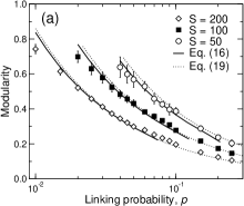
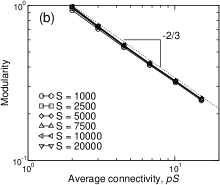
Figure 1: Modularity in Erdös-Rényi random graphs. (a) Comparison of numerical results of the modularity as a function of the linking probability, and the predictions of Eqs. (20) and (23). The numerical results are obtained by maximizing the modularity, Eq. (1), using simulated annealing Kirkpatrick et al. (1983). (b) Modularity as a function of $pS$ for large networks, as predicted by Eq. (20). Both in (a) and (b), numerical problems in the solution of Eq. (9) prevent us from obtaining values of the modularity for larger values of $p$.

In Fig. 1(a), we compare the modularity of ER graphs obtained through optimization of Eq. (1) using simulated annealing Kirkpatrick et al. (1983), with the predictions of Eq. (20). We find good agreement in the relevant region of sparse but connected graphs, that is, $2/S<p\ll 1$.

Equation  (20) enables us to obtain the modularity of large random graphs, something that would not be possible using simulated annealing because of the computational cost. In Fig. 1(b) we show that for $S\rightarrow\infty$ the modularity only depends on $pS$

$$M_{ER}(S\rightarrow\infty,p)\sim(pS)^{-2/3}.$$ (21)

To obtain a closed expression for $M_{ER}$ for any value of $S$, we note that at the percolation point $pS=2$ the random graph contains essentially no loops, that is, the graph is a tree Bollobas (2001). In this case, one can find partitions in which the number of between-module links equals the number of modules $r$ as in the simple one-dimensional case, and the modularity is

$$M_{ER}(S,p=2/S)=M_{1D}(S)=1-\frac{2}{\sqrt{S}}\,.$$ (22)

We propose the simplest ansatz that verifies Eqs. (21) and (22) simultaneously

$$M_{ER}(S,p)=\left(1-\frac{2}{\sqrt{S}}\right)\left(\frac{2}{pS}\right)^{2/3}\,.$$ (23)

In Fig. 1(a), we show that Eq. (23) is in good agreement with values obtained using simulated annealing.

Our analytic treatment allows us to explain the origin of the modularity in random graphs. The typical partition of an ER graph into modules of size $n$ is very unlikely to have a number of within-module links $k_{i}$ larger than the average $pn(n-1)/2$, expected for a random partition of the nodes. However, the number of possible partitions $S!/(n!r)$ is so large that, typically, there exists a partition whose $k_{i}$ is much larger than the average. For example, for a network with $S=200$ and $p=0.02$ one typically finds a partition with $r=7$ modules and $k_{i}\approx 36$, instead of the value $k_{i}\approx 8$ expected for a random partition.

Remarkably, the modularity of a random graph can be as large as that of a graph with modular structure imposed at the onset Girvan and Newman (2002). In such a graph, nodes are divided into modules and each pair of nodes is connected with probability $p_{i}$ if they belong to the same module, and with probability $p_{o}<p_{i}$ otherwise. Using the same example as before, the modularity of an ER graph with $S=200$ and $p=0.02$ is the same as the modularity of a graph with $m=7$ modules, $p_{i}\approx 0.09$, and $p_{o}\approx 0.004$.

Scale-free networks—So far, we have considered $d$-dimensional regular lattices and ER random graphs, in which all nodes have essentially the same degree. However, many complex networks display scale-free degree distributions Albert and Barabási (2002), meaning that some nodes have degrees that are orders of magnitude larger than the average. Since the results presented for ER graphs rely on the fact that there are many partitions of the network and implicitly on the fact that nodes are exchangeable, it is worth asking whether “random” scale-free networks also display modularity.

To answer this question, we use the scale-free model proposed in Barabási and Albert (1999). In the model, the network grows by the addition of new nodes. Each time a new node is added, it establishes $m$ preferential connections to nodes already in the network. In Fig. 2(a), we show the modularity of scale-free networks as a function of the network size $S$ for different values of $m$. As before, we find the modularity by optimizing Eq. (1) using simulated annealing. As for ER graphs, the modularity approaches a finite value for large $S$ and decreases with the connectivity $m$.

We are unable to derive a general expression for the modularity of scale-free networks. However, for $m=1$ the scale-free network is a tree. Thus,

$$M_{SF}(S,m=1)=M_{1D}(S)=1-\frac{2}{\sqrt{S}}\,.$$ (24)

For larger values of $m$, we find numerically that, at a fixed network size, the modularity is a linear function of $1/m$. The simplest possible ansatz for the modularity that verifies this condition and Eq. (24) simultaneously is

$$M_{SF}(S,m)=\left(a+\frac{1-a}{m}\right)\left(1-\frac{2}{\sqrt{S}}\right)\,.$$ (25)

As we show in Fig.2, this approximation works well for $a=0.165\pm 0.009$.

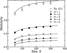
Figure 2: Modularity in scale-free networks. Numerical results of the modularity as a function of the network size $S$ for different values of $m$. These results are obtained by maximizing the modularity, Eq. (1), with simulated annealing. The lines are the predictions of Eq. (25), with $a=0.165\pm 0.009$ in all the cases.

Conclusions— We have shown that modularity in networks can arise due to a number of mechanisms. We have demonstrated that networks embedded in low dimensional spaces have high modularity. We have also shown analytically and numerically that, surprisingly, random graphs and scale-free networks have high modularity due to fluctuations in the establishment of links.

Recently, several works have reported the existence of modules in complex networks and suggested that some evolutionary mechanism must enhance modularity. This statement is based, in the best of the cases, on the fact that the modularity is large enough, and relies implicitly on the assumption that random graphs have low modularity.

Our results enable one to define statistically significant modularity in networks. We argue that, just as it is already done for the clustering coefficient and other quantities, the modularity of complex networks must always be compared to the null case of a random graph. The analytical expressions we have derived provide a convenient way to carry out such a comparison.